A mixed mode function boundary element method for very large floating structure water interaction systems excited by airplane landing impacts

ePrints Soton

Copyright © and Moral Rights for this thesis are retained by the author and/or other copyright owners. A copy can be downloaded for personal non-commercial

research or study, without prior permission or charge. This thesis cannot be

reproduced or quoted extensively from without first obtaining permission in writing from the copyright holder/s. The content must not be changed in any way or sold commercially in any format or medium without the formal permission of the

copyright holders.

When referring to this work, full bibliographic details including the author, title, awarding institution and date of the thesis must be given e.g.

AUTHOR (year of submission) "Full thesis title", University of Southampton, name of the University School or Department, PhD Thesis, pagination

UNIVERSITY OF SOUTHAMPTON

A Mixed Mode Function – Boundary Element Method

for Very Large Floating Structure – Water Interaction Systems

Excited by Airplane Landing Impacts

Jingzhe, JIN

Thesis submitted for the degree of Ph.D.

School of Engineering Sciences, Ship Science

ABSTRACT

Doctor of Philosophy

SCHOOL OF ENGINEERING SCIENCES

SHIP SCIENCE

A MIXED MODE FUNCTION – BOUNDARY ELEMENT METHOD FOR VERY

LARGE FLOATING STRUCTURE – WATER INTERACTION SYSTEMS EXCITED

BY AIRPLANE LANDING IMPACTS

By Jingzhe, JIN

This thesis develops a mixed mode function – boundary element method (BEM) to

analyze the dynamics of an integrated airplane – floating structure – water interaction

system subject to airplane landing impacts.

The airplane and the floating structure are treated as two solid substructures of which the

motions are represented by their respective modal functions. The landing gear system of

the airplane is modelled with a few linear spring – damper units connecting the airplane

and the floating structure. The water is assumed to be inviscid and incompressible and the

fluid motion is irrotational. Under a linear potential theory, the motion of the fluid is

governed by the Laplace equation and the related boundary conditions. A linearised

composite free surface boundary condition and an undisturbed far field (infinity) radiation

condition are considered. The Green function, or kernel, of BEM formulation is a

fundamental solution of the Laplace equation assuming an infinite fluid domain. The

motion of the floating structure and the surrounding fluid are coupled through the wetted

surface interface conditions. The coupled equations of the airplane, the floating structure

and the surrounding fluid are solved using a step by step time integration procedure based

method. A few examples are completed to validate the mathematical model and the

developed computer code. In comparing the available numerical and experimental results

reported in the literature, sound agreements are reached.

It is hoped that the developed method and computer code may be further improved and

modified to provide an engineering tool for the dynamic design of Very Large Floating

Structures (VLFS).

Key words: integrated airplane – VLFS – water system, mixed mode function – boundary element method, VLFS dynamics, airplane landing impacts, transient dynamics,

time integration scheme.

This is my opportunity to say a few words of thanks.

First, I would like to acknowledge the School of Engineering Sciences for the

studentship support enabling me to study in the University of Southampton and engage in

this research.

I would like to thank my supervisor, Professor Jingtang Xing for his strict supervision,

constant support and kind encouragement from the beginning to the end.

I would also like to thank all the colleagues and friends in Ship Science, who have at

times provided individual help and support for me over the past few years. In particular, I

thank Dr. Yeping Xiong, Dr. Shihua Miao, Dr. Weibo Wang and Haitao Wang for

discussing some theoretical, technical and software problems. Dr. Mingyi Tan is thanked

for help in solving computer problems and Simon Lewis is acknowledged for reading and

suggesting modifications to the manuscript.

I also want to thank Hisayoshi Endo from Japan for kindly providing the experimental

data.

I owe a big thankyou to all my friends in Southampton, too many to mention. Without

you, I would have had nowhere to escape from office. Among the others, Lin Ji and

Wenjuan Sun have to get a mention for the times we spent together.

Last but not least, I wish to thank my parents, all my family back in China and my

husband in Norway for their never ending love and support, without which finishing the

1 Introduction ………... 1

1.1 Very Large Floating Structures (VLFS) ………... 1

1.1.1 Overview of VLFS ………... 1

1.1.2 Application of VLFS ………... 3

1.1.3 Characteristics of VLFS ……….. 4

1.2 Hydroelasticity Theory ……… 5

1.3 Frequency Domain Analysis Methods ……… 9

1.3.1 Analysis methods regarding fluid motion ………... 9

1.3.2 Analysis methods regarding structure motion ………... 11

1.3.3 Comparative study of responses of VLFS in waves ……… 13

1.4 Time Domain Analysis Methods ………... 14

1.4.1 Various methods ……….. 14

1.4.2 Summary ………... 17

1.5 Research Aims and Dissertation Contents ……….. 18

1.5.1 Aims ……….... 18

1.5.2 Contents ………... 19

2 Theory Background ………... 21

2.1 Mode Theory of Structural Dynamics ………... 21

2.1.1 Equation of natural vibrations ………... 21

2.1.2 Solutions of natural vibration ……….. 22

2.1.3 Orthogonality of natural modes ………... 23

2.1.4 Different approaches to obtain natural modes ………... 25

2.1.5 Modal superposition method ………... 30

2.2 Time Integration Schemes ………... 32

2.2.1 The central difference method ………... 33

2.2.2 The Houbolt method ……… 35

2.2.3 The Wilson θ method ……… 36

2.2.4 The Newmark method ………... 37

2.3 Basic Theory of Hydrodynamics ………... 39

2.3.1 Governing equation ………... 39

2.3.2 Bernoulli’s theorem ………... 41

2.3.3 Boundary conditions ……….... 44

2.4 Boundary Element Method ………... 47

2.4.1 Basic concepts ………... 47

2.4.2 Formulation of boundary integral equation ………... 50

2.4.3 Numerical solution ……….. 52

3 Modelling of Landing Gear System of Airplane ……….... 55

3.2 Modelling of Landing Gear System of Airplane ……….. 59

3.2.1 General description ……….. 59

3.2.2 Coefficients of linear spring – damper system ……….... 59

3.3 Simulation of a Drop Test ……… 63

4 Mixed Mode Function – Boundary Element Method ……….. 68

4.1 General Description ………... 68

4.2 Governing Equations ………... 71

4.2.1 Fluid domain ……… 71

4.2.2 Floating structure and airplane ……… 73

4.2.3 Coupling conditions on fluid – structure interaction interface ………… 75

4.2.4 Initial conditions ……….. 76

4.3 Mode Equations of Solid Substructures ……….. 77

4.3.1 Mode equations of floating structure and airplane ……….. 77

4.3.2 Coupled equation of two substructures ………... 80

4.4 Boundary Element Equation of Fluid Domain ……….... 81

4.5 Mixed Mode Function - Boundary Element Equation ……….... 84

5 Time Integration Scheme ………... 87

5.1 Solution Procedure ……….. 87

5.2 Stability and Accuracy Analyses ………... 91

5.2.1 Selection of parameters α and δ ……… 92

5.2.2 Selection of time step Δt ………... 93

6 Program Implementation ………... 94

6.1 Introduction of Program MMFBEP ………... 94

6.2 Function of Program MMFBEP ……….. 95

6.3 Structure of Program MMFBEP ……….. 96

6.4 Characteristics of Program MMFBEP ………... 98

6.5 User Manual of Program MMFBEP ………... 100

6.5.1 Write input file INPUTP.DAT ………... 100

6.5.2 Generation of input file INPUTM.DAT ……….. 103

6.5.3 Contents of output file ………... 105

7 A Mass–Spring–Damper System Dropping onto a Floating Mass ….. 107

7.1 General Description ………... 108

7.2 Numerical Simulation ………. 109

7.2.1 Simulation in 2D fluid domain ……….. 109

7.2.2 Simulation in 3D fluid domain ……….. 110

7.3 Validation ………... 110

8.2 A Car Running Test ………..………. 121

8.2.1 Description ……… 121

8.2.2 Execution of program MMFBEP ……….. 123

8.2.3 Results and discussions ………. 123

8.3 Landing Beam – Floating Beam – Water Interaction System ………….……... 125

8.3.1 Description and program execution ……… 125

8.3.2 Results and discussions ………. 126

9 An Airplane Landing onto a Floating Structure ……… 140

9.1 General Description ………... 140

9.2 Modelling of the System ……… 142

9.2.1 Model of Boeing 747-400 airplane ………... 142

9.2.2 Linearization of landing gear system ……… 145

9.2.3 Model of floating structure ……… 149

9.2.4 Truncation of fluid domain ……… 153

9.3 Results and Discussions ……… 153

10 Conclusions and Future Work ………... 175

10.1 Conclusions ……… 175

10.2 Future Work ……… 177

References ……… 178

Publications ……… 189

Appendix A ……… 190

. Appendix B: Program MMFBEP ……… 192

Appendix C: Input file INPUTP.DAT for Landing Beam–Floating Beam– Water Interaction System in 2D Fluid Domain ……….. 227

Appendix D: Input file INPUTM.DAT for Landing Beam–Floating Beam– Water Interaction System ………...………….. 233

Figure 1.1 A pontoon type floating airport (Isobe 1999)………2

Figure 1.2 A semi-submersible type MOB (Remmers et al 1999)………...2

Figure 1.3 Structure of thesis………20

Figure 2.1 A uniform beam with free – free ends……….27

Figure 3.1 Oleo – pneumatic shock absorber………...57

Figure 3.2 Efficiency diagram of landing gears………58

Figure 3.3 Simplified landing gear model ………59

Figure 3.4 Mass – spring – damper system used to simulate the drop test………..63

Figure 3.5 Measured acceleration at the CG position of landing gear carriage...66

Figure 3.6 Calculated acceleration of mass – spring – damper system……….………...66

Figure 3.7 Measured grounding force – CG position of landing gear carriage …………66

Figure 3.8 Calculated spring – damper force – CG position of mass – spring – damper system………..67

Figure 4.1 An integrated airplane - floating structure - water interaction system subject to airplane landing impact………...69

Figure 5.1 Flow chart of the time integration scheme………..92

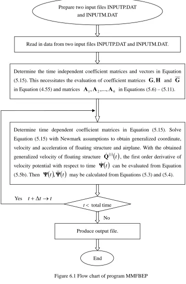
Figure 6.1 Flow chart of program MMFBEP………...98

Figure 6.2 Numbering of nodes and elements for floating structure……….104

Figure 7.1 A mass – spring – damper system dropping onto a floating mass…………108

Figure 7.2 Added mass and damping coefficients for a family of 2D rectangular cylinders Vugts (1968)………..112

Figure 7.3 A mass – spring – damper system dropping onto another mass – spring – damper system………...113

Figure 7.4 Time history of the displacement of the dropping mass………..……..116

Figure 7.5 Time history of the displacement of the floating mass………116

Figure 7.6 Time history of the velocity of the dropping mass………..117

Figure 7.7 Time history of the velocity of the floating mass………117

Figure 7.8 Time history of the acceleration of the dropping mass………...118

Figure 7.9 Time history of the acceleration of the floating mass……….118

Figure 7.10 Time history of the interaction force from the spring – damper unit……..119

Figure 7.11 Time history of the force from water pressure applied on the floating mass………...119

Figure 8.1 A landing beam - floating beam - water interaction system subject to landing impacts………..121

Figure 8.2 Arrangements of displacement measure points and car moving rail on the plate model………122

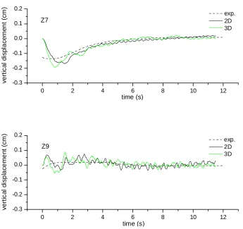
Figure 8.3 Time histories of the vertical displacement measured at the five points on the plate model………125

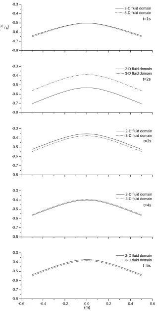
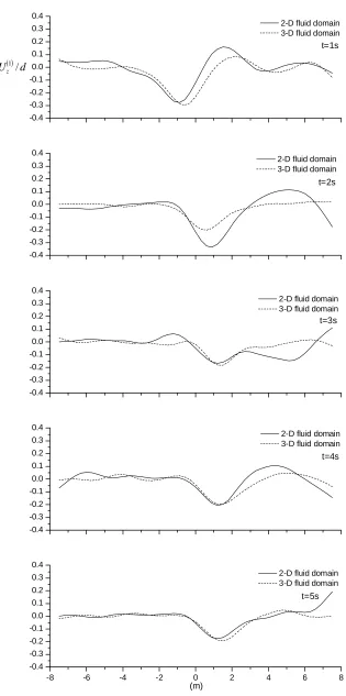
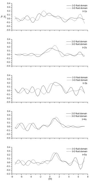
Figure 8.6 Distribution of the non – dimensional water pressure along the 15m floating

beam at time t =1,2,3,4,5s……….132

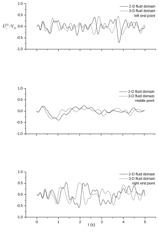
Figure 8.7 Time histories of the non – dimensional vertical displacement at the left end and middle point of the landing beam………...…………133

Figure 8.8 Time histories of the non – dimensional vertical velocity at the left end and middle point of the landing beam………123

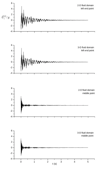
Figure 8.9 Time histories of the non – dimensional vertical acceleration at the left end and middle point of the landing beam……….134

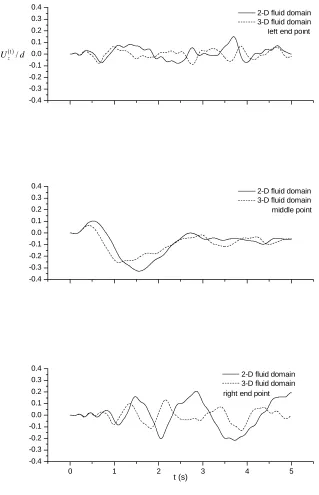
Figure 8.10 Time histories of the non – dimensional vertical displacement at the left end, middle and right end point of the floating beam……….135

Figure 8.11 Time histories of the non – dimensional vertical velocity at the left end, middle and right end point of the floating beam……….136

Figure 8.12 Time histories of the non – dimensional vertical acceleration at the left end, middle and right end point of the floating beam……….137

Figure 8.13 Time histories of the non – dimensional water pressure at the left end, middle and right end point of the floating beam………...138

Figure 8.14 Time history of the non – dimensional relative displacement between the two elastic beams at the supporting system……….139

Figure 8.15 Time history of the non – dimensional interaction force provided by the supporting system………139

Figure 8.16 Time history of the non – dimensional resultant vertical force from induced water pressure………..139

Figure 9.1 A Boeing 747-400 jumbo plane landing on a floating structure…...………141

Figure 9.2 Boeing 747-400 jumbo plane (BOEING webpage)……….……142

Figure 9.3 Simplified model of Boeing 747-400 jumbo plane………...143

Figure 9.4 First ten modes of airplane model……….148

Figure 9.5 Model of floating structure………149

Figure 9.6 Ten picked modes of floating structure……….152

Figure 9.7 Distribution of the displacement of airplane at time t=11s…………...156

Figure 9.8 Distribution of the deformation of floating structure at five distinct times ………...158

Figure 9.9 Distribution of water pressure along the floating structure at five distinct times….……….160

Figure 9.10 Time histories of the deformation at the five nodes of the airplane………161

Figure 9.11 Time histories of the vertical velocity at the five nodes of the airplane….162 Figure 9.12 Time histories of the vertical acceleration at the five nodes of the airplane ………...163

Figure 9.13 Time histories of the deformation of floating structure at the ten selected nodes F1 – F10……….……….165

Figure 9.16 Time histories of water pressure of floating structure at the ten selected nodes

F1 – F10………..……….……….171

Table 3.1 Parameters of landing gear………64

Table 6.1 Subroutines of program MMFBEP………...99

Table 8.1 Particulars of the floating plate model……….122

Table 9.1 Basic parameters of Boeing 747-400 airplane (BOEING webpage)……...143

Table 9.2 Parameters of beams used to model Boeing 747-400 airplane………144

Table 9.3 Frequencies of the first ten modes of the airplane model………145

Table 9.4 Parameters of the landing gears of Boeing 747-400 airplane………..148

Table 9.5 Coefficients of the four linear spring-damper units………149

Table 9.6 Parameters of floating structure (Kashiwagi 2004)……….149

a added mass coefficient representing hydrodynamic force

a static stroke parameter of the landing gears

11 1,...,a

a coefficients used in the time integration scheme

x

a horizontal acceleration of the airplane in landing

A amplitude of a harmonic motion

CG

A acceleration at centre of gravity

6 1,. ..,A

A coefficient matrices and vectors used in expressing first order derivative

of velocity potential with respect to time

6 1,. ..,A

A matrices and vectors truncated from A₁,. ..,A₆

b damping coefficient representing hydrodynamic force

1, ..., 4

b b constants to determine the spatial function Φ

( )

5, 6

b b constants to determine the function f

( )

B width of the floating structure

1, 2

B B constants to determine the displacement xˆ of the mass–spring–damper

system relative to equilibrium position

0, 1

c c constants to be determined for the Green function G

( )

C damping coefficient of spring – damper unit

) 4 ,..., 1 (J =

C_J damping coefficients of the four landing gears

l

C constant value of the Bernoulli function along a streamline

C damping matrix of a structure

11, 12, 21, 22

C C C C component damping matrices in the coupled equation of the two

substructures

C generalized damping matrix of a structure

d mean draft of the floating structure

E′ kinetic energy caused by the sink velocity of landing gear carriage ( )

₍

₎

2 , 1 = I

E I

EI bending stiffness of a structure

( )

f a function of time

e

f frequency of external excitation force

) 4 ,..., 1 (J =

f_J force provided by the four landing gears

) , , , (x y z t

F free surface function

F′ force provided by spring – damper unit

d

F damping force applied to a harmonic system

w

F resultant force from water pressure applied on the floating structure

x

F constant landing resistance

F external force applied on a structure ( )1

d

F generalized force from water pressure applied on the floating structure ( )2

d

F generalized force from the inertia of the airplane ( )

₍

₎

2 , 1

= I I g

F generalized force from the gravity of the floating structure and airplane ( )I

₍

₎

i

F generalized force from the landing gear system

Fˆ a vector

F body force per unit mass

g acceleration of gravity

) 2 , 1 (

) (I _I =

g external force applied on the floating structure and airplane

( )

G Green function of fluid domain

1, 2, 3

G G G coefficient matrices to determine the generalized force from water

pressure ( )1

d

F

4

G coefficient matrix in the coupled fluid – structure interaction equation

G,H,G coefficient matrices in the boundary element equation

H Bernoulli function

i = −1

k j

i, , unit vector along three coordinate axes ( )I

₍

₎

I unit diagonal matrix of order M( )I

(

)

1

k equivalent spring coefficient at static stroke of the landing gear

2

k equivalent spring coefficient at working stroke of the landing gear

K spring coefficient of spring – damper unit

) 4 ,..., 1 (J =

K_J spring coefficients of the four landing gears

K stiffness matrix of a structure

11, 12, 21, 22

K K K K component stiffness matrices in the coupled equation of the two

substructures ( )I

₍

₎

K generalized stiffness matrices of the floating structure and airplane

K generalized stiffness matrix of a structure

M C

K~ ,~ ,~ coefficient matrices in the effective stiffness matrix

L length of the floating structure ( )1

m total mass of the floating structure ( )2

m total mass of the airplane

m mass per unit length of a beam

M number of retained modes

M′ mass sustained on one landing gear ( )

₍

₎

M I

number of retained modes of the floating structure and airplane

M mass matrix of a structure ( )I

₍

₎

M generalized mass matrices of the floating structure and airplane

M generalized mass matrix of a structure

n outward normal of fluid domain

n′ load factor of landing gear

n unit outward normal vector of a closed surface

N number of degrees of freedom

f

N number of element on the free surface

∑

N number of element on the wetted interaction interface

f

N element identifying number on the free surface

∑

P water pressure

a

P atmospheric pressure at the free surface

s

P static load on landing gear

w

P load on landing gear at working stroke ( ) ( ) ( )

) , ,

(x_q1 y_q1 z_q1

q source point in fluid domain

q natural mode vector of a structure

Q generalized coordinate vector of a structure ( )I

₍

₎

Q generalized coordinates of the floating structure and airplane

r distance between field and source points

R R

R_a , _v , coefficient vectors in the effective load vector

S =Γ_f +Γ_∞ +Γ_b +∑

s

S static stroke of the shock absorber of landing gears

w

S working stroke of the shock absorber of landing gears

t time

t

Δ time step used in the time integration scheme cr

t

Δ critical time step

T thickness of the floating structure

e

T period of the external excitation force

n

T smallest period of a system

( )

u , vertical displacement of a beam

u displacement vector of a structure

U a potential function ( )2

0

U initial deformation of the airplane ( )

₍

₎

1,2

= I I

U displacement vector of the floating structure and airplane

V amplitude of fluid velocity

V volume enclosed by a closed surface

n

V velocity of floating structure along the outward normal of wetted surface

(

)

V velocity vector of fluid

(

)

0 Vx ,0, Vz

V initial landing velocity of the airplane

W work done by the damping force of a harmonic system in one cycle

d

W dissipated energy within one stroke of shock absorber

xˆ displacement of mass–spring–damper system relative to equilibrium

position

x

~ _{displacement of a harmonic motion}

x a field point on the boundary of the fluid domain

x′ a source point on the boundary of the fluid domain

Xˆ displacement of mass–spring– damper system relative to initial position

X a field point inside the fluid domain

X′ a source point inside the fluid domain

α ,δ parameters from Newmark assumptions β

α, coefficients of Rayleigh damping β′ phase angle of a harmonic motion

b

Γ sea bed boundary

f

Γ free surface boundary

∞

Γ far field boundary ij

δ Kronecker delta function

( )

Δ Dirac’s delta function

ε radius of a spherical control surface ε′ damping ratio

( )

₍

₎

2 , 1

= I I

ε strain vector of the floating structure and airplane

) , , (x y t

ς vertical elevation of free surface

η energy absorption efficiency of the shock absorber of landing gears ( )I

₍

₎

η material damping factor of the floating structure and airplane

structure and airplane ( )I

₍

₎

μ Poisson’s ratio of the floating structure and airplane ( )

₍

₎

2 , 1

= I I

ν unit outward normal vector of the floating structure and airplane

ξ modal damping parameter π ratio of circumference to diameter ρ mass density of water

( )

) 2 , 1 (I =

I

ρ mass density of the floating structure and airplane ( )I _{(I =1,2)}

σ stress vector of the floating structure and airplane

τ a small increase of time ( ) ( ) ( )

(

)

φ velocity potential of fluid

φ′ transfer coefficient of landing gears

( )

Φ a spatial function

Φ modal matrix of a structure ( )I

₍

₎

Φ normal natural mode matrices of the floating structure and airplane

χ energy dissipation coefficient of landing gears ψ a potential function

Ψ velocity potential vector

n

Ψ vector of normal derivative of velocity potential

Ψ truncated velocity potential vector along the wetted interface

ω frequency of a harmonic motion ( )I

₍

₎

ω = natural frequency of the floating structure and airplane

d

ω frequency of a damped motion

t

ω truncation frequency ( )1

Ω floating structure ( )2

Ω airplane structure f

Ω fluid domain

∑ wetted interaction interface

Π a scalar function ∇ Hamilton operator

2

∇ Laplace operator

Notations for Coordinate Reference Axes and Key Points

( )1 _x( ) ( ) ( )1 _y1_z1

o − a Cartesian coordinate system fixed in space ( )2 _x( ) ( ) ( )2 _y 2 _z 2

o − a moving Cartesian coordinate system ( )1 _X( ) ( ) ( )1_Y 1_Z 1

O − Lagrangian coordinate system of the floating structure ( )2 _X( ) ( ) ( )2_Y 2 _Z 2

O − Lagrangian coordinate system of the airplane ( )1

(

)

, , _{c c} c

c x y z

x position of the mass centre of the airplane ( )

(

)

0 1

0 1

0 1

0 c , c , c c x y z

x initial position of the mass centre of the airplane ( )

(

)

₍

₎

2 1, ,

,Y Z I =

X I I I

I

X a material point of the floating structure and airplane ( )

(

)

₍

₎

1,...,4

, , 1 1

1

1 _{X Y Z J} =

J J J J

X landing gear position on the floating structure ( )

(

)

₍

₎

4 ,..., 1 ,

, 10 1 0 1

0 1

0 XJ YJ ZJ J = J

X initial position of the landing gears on the floating

structure ( )

(

)

₍

₎

1,...,4

, , 2 2

2

2 _{X Y Z J} =

J J J J

Chapter 1

Introduction

1.1

Very Large Floating Structures (VLFS)

1.1.1 Overview

of

VLFS

It is well known that seventy percent of the earth surface is covered by water, which

contains abundant resources, such as: chemicals, minerals, natural gas, oil, etc. Marine

resource exploitation has always been an important task for future developments. Together

with the growing population and the corresponding expansion of urban areas in land-scarce

countries and countries with long coastlines, interest in utilising ocean space has increased

constantly in recent years. As a consequence, the concept of Very Large Floating Structures

(VLFS) was proposed. Such structures can serve as a sea base where various operations

and activities are carried out.

The original concept of VLFS seemed to be “the huge metal vessel” described by the

19th century French novelist, Jules Verne, in his science fiction “Twenty Thousand Leagues

Under the Sea” (ISSC 2006). The first VLFS promoted in earnest was the Armstrong

Seadrome proposed initially to enable airline routes across the world’s oceans (Armstrong

1924).

The VLFS concept has not been taken into serious consideration until the potential of

modern shipbuilding technology became apparent in the 1950s (ISSC 2006). Before then

the only manner in which ocean space could be exploited on a large scale was through land

reclamation. Such exploitations are limited to shallow regions of the continental shelf.

In the 1950s, architects were drawn to the idea of large floating structures. This new

research interest was reflected through the proposal of a floating airport for the new Kansai

International Airport in 1973 (ISSC 2006) and the semi-submersible unit of a floating city

at the Okinawa International Ocean Exhibition in 1975 (ISSC 2006). Since the early 1970s

VLFS is a unique concept of ocean structures primarily because of its unprecedented

length (103-104 m), displacement (106-107 tons), cost (5-15 billion $US) and the associated

analysis methods and design procedures (ISSC 2006). There are two basic VLFS hull

types.

1) Pontoon type: a complex of pontoon hulls designed for operation in protected waters,

also known as Mega-Float. A pontoon type floating airport is shown in Figure 1.1.

2) Semi-submersible type: a complex of semi-submersible hulls designed for operation

in deeper water and/or open sea. The semi-submersible hull may be an array of columns, or

it may be a system of columns resting on submerged pontoons. A semi-submersible type

Mobile Offshore Base (MOB) is depicted in Figure 1.2.

Figure 1.1 A pontoon type floating airport (Isobe 1999)

1.1.2 Application

of

VLFS

VLFS may be applied to serve many different purposes in reality. A few examples of

these applications are listed below, among the others (ISSC 2006).

1) Airport

Due to the limited land space near to the coastlines of densely populated areas, there will

be a need in the future for floating airports. A floating airport can reduce pollution and

noise level in the surrounding residential areas compared to a land based airport.

2) MOB

MOB is mainly for military application. It can be assembled/disassembled on the site of

military operations. A similar concept may be envisaged for a mobile emergency rescue

base to support humanitarian relief operations worldwide.

3) Offshore port facilities

Offshore container terminals are being considered to service large ocean-going vessels.

It will be beneficial to site offshore terminals for potentially hazardous vessels, such as

LNG ships.

4) Offshore storage and waste disposal facilities

In the densely populated coastal regions, setting up offshore storage facilities, waste

processing and treatment plants is very attractive. Examples of offshore storage facilities

exist in Japan, where two of the nation’s ten national oil stockpiles are floating stockpiles

sited off the islands of Kamigoto (1988) and Shirashima (1996) respectively.

5) Energy islands

Depending on the prevailing climate, an offshore energy facility may include wind

turbines, wave power generators, tidal current turbines and ocean thermal energy

conversion units.

6) Habitats

Considering the pressure on coastal zones from the growing population and the threat of

environmental changes, offshore habitats may provide a solution for the future. There are

current proposals for offshore sports facilities and theme parks in Japan and South Korea

Among all these applications of VLFS, a floating airport is one of the important research

areas. Proposals to use floating structures for airplane landing/take-off were first

considered in the 1920s (Armstrong 1924). These concepts were investigated more

seriously for military applications by the US in the 1940s and a demonstration project was

built and tested successfully in 1943 (ISSC 2006). In recent years, due in large part to the

efforts of the Technological Research Association of Mega-Float (TRAM) in Japan, the

fundamental design and construction needs of a floating airport have been extensively

studied. Numerical analysis methods were developed alongside an experimental

programme carried out by TRAM, which resulted in the construction of a 1000m by 60m

technology demonstrator. Although a floating airport has yet to be approved for

construction in reality, research interest regarding it remains strong.

1.1.3 Characteristics

of

VLFS

The engineers will face profound challenges regarding the design and construction of

VLFS, as they are different from conventional ship and offshore structures. VLFS have the

following characteristics (ISSC 2006):

1) Large size

VLFS are unprecedented large structures. Due to the large length/depth ratio, they are

very flexible thus the elastic response is dominant for VLFS. Consequently, hydroelastic

analysis becomes necessary for estimating the response of VLFS under waves and other

external loadings.

2) Environment condition

Physical environmental conditions in which VLFS must operate may not be simply

considered spatially uniform in the sense that coherence of environmental conditions such

as wind, wave and current must be considered.

3) Connection at sea

VLFS are modularized structures. In the assembly of VLFS, base modules/units need to

be joined together at sea. Control of thermal deformation and alignment of units are key

4) Positioning

Reliability of the station keeping system is crucial to the operational availability of

VLFS. In general, station keeping of MOB is accomplished by Dynamic Positioning

System (DPS) and that of Mega-Float is accomplished with dolphin moorings.

5) Design life

Design life is typically 50 years for MOB and 100 years for Mega-Float. These criteria

are substantially greater than those for conventional ship and offshore structures.

6) Model test

As there is no experience in designing such huge floating structures, model test plays an

important role in clarifying key issues of the hydroelastic responses of VLFS. How to set

up and carry out model tests in the current towing tank and ocean basin facilities is itself a

new experimental technology.

When considering the characteristics of a floating airport, the following aspects are

recognized. The problem of an airplane landing/take-off from a floating structure

necessitates interdisciplinary studies relating the airplane, the floating airport and the

surrounding fluid. Solving this problem requires a knowledge of structural dynamics,

hydrodynamics and hydroelasticity theory. It is also a transient problem due to the time

dependent landing/take-off impacts of the airplane, thus solutions need to be obtained in

the time domain. The airplane and the floating airport are connected through the landing

gear system, whose mechanics is entirely nonlinear. This nonlinearity will increase the

computation efforts significantly, unless a proper linearization scheme is applied.

1.2

Hydroelasticity Theory

Hydroelasticity is concerned with the phenomena involving mutual interactions among

inertial, hydrodynamic and elastic forces (Heller & Abramson 1959). The interaction

between fluid pressure and structural deformation is the key point in classifying a problem

as hydroelastic.

hydroelasticity as the fluid pressure acting on the wetted surface of the structure will

induce both rigid-body motion and structural distortion and in return the rigid-body motion

and distortion of the structure will disturb the pressure field, flow and wave pattern of the

surrounding fluid. However, for most traditional marine structures such as ships and

platforms, the distortion of these structures is so small in comparison with their rigid body

motions that the effect of the elastic distortion of the structure on the fluid field can be

neglected. The hydrodynamics book of Newman (1977) contributed a fundamental

theoretical approach to the problems of ship – water interactions. Within this theory, the

structure is assumed to be a rigid body for the determination of the water pressure acting

on the wetted surface. The distortion of the structure can be calculated by applying either

the distributed pressure or the resultant integrated global forces acting on the structure in a

subsequent structural analysis.

Although the concept that floating structures behave like elastic bodies has been

accepted, hydroelastic analysis hasn’t been brought into the scope of marine technology

until the 1970s when Bishop (1971) suggested that ship response could be evaluated based

on hydroelasticity theory. This was then followed by the development of “wet modes”

method employed by Bishop et al (1973) and Bishop & Eatock Taylor (1973) to determine

symmetric stress and structural dynamics of ship hulls in waves. The idea of the “wet

modes” method was that dynamic characteristics of the ship hull were to be determined

after both structural properties and fluid actions had been taken into account. On the other

hand, Bishop & Price (1974) introduced the use of “dry modes” method in which the

modal analysis of a ship hull is carried out in vacuo and the influence of the surrounding

fluid is treated as external loadings of the ship hull. Bishop & Price (1976) later discussed

comparisons between these two approaches.

The hydroelasticity theory was originally described for two dimensional (2D) cases

based on the “dry modes” method. The ship hull was assumed to be a “beamlike” structure

whose dynamic characteristics in vacuo were determined in a “dry hull analysis” in the

absence of any damping or external forces. The fluid field was represented by strip theory.

hydrodynamic forces, which formed a preliminary step for the dynamic response analysis

of a symmetric ship subject to waves (Bishop et al 1977). Later Bishop et al (1980) studied

the asymmetric responses of a container ship in regular waves. The study on asymmetric

offshore structures or ships with an angle of heel was brought into scope by Conceicao et

al (1984). The detailed theory of 2D hydroelasticity was established in a well known book

“Hydroelasticity Theory of Ships” (Bishop & Price 1979).

The application of the 2D hydroelasticity theory is limited to slender or beam-like

structures. In order to examine the fluid-structure interaction behaviour of non-beamlike

structures, Wu (1984), Price & Wu (1982,1983,1986) and Bishop et al (1986a) presented a

general linear three dimensional (3D) hydroelasticity theory of floating structures moving

in a seaway. In this theory, a linear finite element approach is used to describe the dynamic

behaviour of the 3D dry structure in vacuo. The singularity distribution method was used to

determine the fluid actions associated with the distorting 3D wetted structure.

Most of the early studies were undertaken in the frequency domain assuming time

harmonic motion of the structure. However, transient phenomena observed in

fluid-structure interactions of ships and other floating structures, such as whipping induced

by slamming, transient responses due to aircraft landing/take-off, underwater explosion,

dynamic capsizing, collision and grounding can only be studied in the time domain. Gu et

al (1989) and Xia & Wang (1997) described a time domain strip theory and used it to study

the vertical motion and longitudinal bending of a ship. The associated linear hydrodynamic

forces were formulated in terms of time convolutions and the structure was treated as a

Timoshenko beam. Janardhanan et al (1992) developed a 3D time domain approach,

incorporating time history effects and nonlinear fluid loading from wave effects. In his

method the fluid field was represented in terms of the frequency domain Green function.

Wu & Moan (1996) and Wu et al (1996) reported a time domain hydroelastic analysis for

ships at high forward speed. Wang (1996) and Wang & Wu (1998) presented a time domain

3D hydroelasticity method for ships advancing in waves. In their method the time domain

Green function (Liapis & Beck 1985) and the impulsive response function were employed.

involving the hydrodynamic loading and the structure response have to be addressed.

Bishop et al (1978) and later Belik et al (1980) were among the first to use modal analysis

to predict the transient responses due to slamming in regular head waves, using impact and

momentum slamming theories. This was then extended by Belik & Price (1982) and Belik

et al (1983) to study slamming responses in irregular head waves. Faltinsen (1996) studied

the bottom slamming of a floating airport and later provided an overview on hydroelastic

slamming Faltinsen (2000). Faltinsen states that “when the angle between the impacting

free surface and the body surface is small, hydroelasticity has to be considered and the

importance of hydroelasticity depends on the impact velocity and the highest natural period

of the local structure”. Maeda et al (1997) and Ikoma et al (1998) calculated the

second-order wave loads acting on large floating structures. Chen et al (2003a) studied the

motion of a moored floating body with the consideration of second order fluid forces

induced by the large rigid body rotations in high waves, the variation of the instantaneous

wetted surface and the coupling of the first order wave potentials. The hydroelastic

responses of a structure manoeuvring in viscous fluid were prescribed by Du (1999). With

regards to the structural nonlinearity, Chen et al (2003b) proposed a method for analyzing

the hydroelastic characteristics of VLFS in multidirectional monochromatic incident waves

taking into account the effect of the membrane forces.

The 2D and 3D hydroelasticity theory has been widely used by many researchers to

investigate the hydrodynamic/hydroelastic behaviour of floating structures since they were

proposed. Bishop et al (1986b) and Price et al (1987) predicted hydroelastic behaviour of a

SWATH (Small Water Area Twin Hull). Fu et al (1985,1986,1987) studied the towage of a

jack-up. Price et al (1988) applied the theory to a submerged flexible cylindrical shell.

The 1990s has seen more and more application of hydroelasticity theory into the

dynamics of VLFS. The huge length/draught ratio makes VLFS very flexible. This causes

significant wave – structure interactions and therefore a hydroelastic analysis is necessary.

One of the essential steps in the design stage is to estimate the hydroelastic wave induced

responses of VLFS and the influence of other external loadings to guarantee structural

over many years. The main research publications on this subject may be divided into two

categories: frequency domain analysis methods and time domain analysis methods. Each

approach is considered in turn next.

1.3

Frequency Domain Analysis Methods

When the motions of VLFS and the surrounding water are time harmonic, they can be

analyzed in the frequency domain. The relevant analysis methods are known as frequency

domain methods. In this case it is the amplitudes of the motions that is to be determined.

This section provides a brief review on the frequency domain analysis methods for

pontoon type VLFS. Practical calculations of the responses of VLFS in regular waves have

been attained and fundamental characteristics of the responses are also clarified (Ohmatsu

1998a, Iwahashi et al 1998). As a result, the wave induced hydroelastic responses of VLFS

can now be predicted with good accuracy in the frequency domain within a linear regime.

There exist a large number of publications involving frequency domain analysis. The

interested readers may start from the following review papers to obtain a general idea of

the existing analysis methods, which include a Report of the Special Task Committee on

VLFS (ISSC 2006), Ohmatsu (2005), Chen et al (2006), Watanabe et al (2004), Cui (2002),

Cui et al (2001) and Kashiwagi (2000a).

1.3.1 Analysis methods regarding fluid motion

In general, the surrounding water is assumed to be inviscid, incompressible and the fluid

motion is irrotational. Therefore, the potential flow theory is valid. The governing equation

of fluid motion is the Laplace equation together with suitable boundary conditions. This

problem is often solved by using a boundary element method (panel method) or

eigenfunction expansion-matching method (domain decomposition method).

BEM may be further classified as either direct or indirect. In the direct BEM (Yasuzawa

et al 1997), both the velocity potential and its spatial derivatives are used in the boundary

potential is expressed in terms of a fictitious source distribution function. Yago & Endo

(1996), Yasuzawa et al (1996) and Hamamoto et al (1997) independently developed a

method to determine the water pressure distribution using a BEM. Ohkusu & Namba (1996)

and Namba & Ohkusu (1999) introduced the modified Green function approach, which

corresponds to a modified free surface condition to reflect the presence of a floating plate.

Initially they considered an infinitely long plate, and later the method was extended to a

finite 3D problem.

In conventional BEM (low order BEM), the submerged surface of the floating structure

is represented by a number of small quadrilateral plane elements, and the velocity potential

is assumed to be constant over each element. As the wave length of the incident wave is

much smaller than the length of the floating structure, the number of elements required for

sufficient accuracy is very large, which makes the conventional BEM very time consuming.

Newman & Lee (2002) described two methods to overcome the problems experienced in

the conventional BEM. One is a higher-order method of which the geometry shapes of the

submerged surface are represented exactly or approximated to a high degree of accuracy

using B-spline functions, and the velocity potential is also approximated by B-splines. For

the same accuracy, the number of unknowns in higher-order methods is less than that used

in the low-order methods. As a result of this, the required memory space and computational

time are reduced whilst the accuracy and continuity of the solution are improved.

Higher-order boundary element methods are also used by Yasuzawa et al (1996),

Hamamoto et al (1998) and Utsunomiya et al (1998). The other development is to use the

pre-corrected Fast Fourier Transform method (pFFT) to improve the efficiency of

conventional BEM. pFFT was developed by Phillips & White (1997) for electro-static and

electro-dynamic applications and subsequently extended to the analysis of wave-body

interactions by Korsmeyer et al (1999).

In the eigenfunction expansion-matching method, the entire fluid domain is divided into

an inner domain covered by VLFS and an outer domain. Velocity potential within each

sub-domain is approximated by using the vertical orthogonal eigenfunction expansion and

is forced to match each other on the interfaces of the sub-domains. Ohmatsu (1997, 2001)

surface integral for the hydrodynamic force calculation was simplified to a line integral

with a significant reduction of computation time. Seto & Ochi (1998) and Seto et al (2003)

used a hybrid finite/infinite element formulation for the fluid flow based on the

eigenfunction expansion-matching method. The inner and outer fluid sub-domains were

discretised with planar finite elements and hybrid infinite elements, respectively. Kim &

Ertekin (1998) introduced the eigenfunction expansion-matching method into the fluid

region beneath VLFS. They also efficiently utilized the representation of solutions of the

Helmholtz equation for rectangular regions.

In Kim & Ertekin (2002) and Ertekin & Kim (1999), the governing fluid motion

equations are based on the linear level I Green-Naghdi equations (Green & Naghdi 1976).

The velocity fields in regions with and without the plate were matched using the continuity

of mean mass flux and pressure. The resulting Helmholtz equations were solved by the

boundary-integral-equation method and the finite difference method was used for

discretizing the boundary conditions at the edges of the floating structure. Xia et al (2004)

further studied the nonlinear hydroelasticity of VLFS with the nonlinear, Level I Green-

Naghdi theory.

The fluid motion can also be dealt with Finite Element Method (FEM) based on the

variational principle. Watanabe & Utsunomiya (1996) and Kyoung et al (2006) employed

FEM for solving fluid motion. Although the methods proposed in these two papers are for

time domain analysis, the treatment for fluid domain can obviously be adopted in a

frequency domain analysis.

1.3.2 Analysis methods regarding structure motion

VLFS are generally steel or concrete structures and they are often modeled as elastic

plates, shells or sandwich-grillages in the primary design stage. FEM is often used for the

structural analysis of VLFS. Alternatively, the differential motion equation of VLFS can be

solved using a finite difference scheme.

The motion of VLFS can be solved by either direct or modal superposition method. The

means that a large amount of memory space and CPU time is required. Mamidipudi &

Webster (1994) used the direct method for VLFS. In their solution procedure, the

deflection of VLFS was determined by solving the combined hydroelastic equation via the

finite difference scheme and the hydrodynamic aspects were considered by the panel

method. Their method was modified by Yago & Endo (1996) who applied the pressure

distribution method (Yamashita 1979) for fluid and the equation of motion of VLFS was

solved using FEM.

In the modal superposition method, the motion of VLFS is represented in terms of the

dry or wet natural modes. Compared to the direct solution method, the modal superposition

method is more efficient. However, it is important to judge the effectiveness and rationality

of the mode truncation technique. Takaki & Gu (1996) and Lin & Takaki (1998a)

calculated numerically the dry modes of the structure using FEM. Maeda et al (1995), Wu

et al (1995), Nagata et al (1998), Utsunomiya et al (1998) and Ohmatsu (1998a) employed

the simple products of free-free beam modes as the modal function of rectangular plates

with free edges, which are analytically given and thus able to avoid numerical

differentiations and integrations. Lin & Takaki (1998b) showed that the B-spline functions

can also be used to approximate the modal functions of a plate. Wang et al (2001) adopted

2D polynomial functions as modal functions for the structure. It should be remarked that

all the modes aforementioned are of a dry type. While most analysts use the dry-mode

approach, because of its simplicity and easy accessibility, Hamamoto et al (1996) and

Hamamoto & Fujita (2002) conducted studies using the wet-mode approach.

Based on the modal superposition method for solving the motion of a structure,

Kashiwagi (1997) proposed an effective calculation scheme for computing wave forces on

an elastic plate in the regime of very short wave-lengths. The scheme employed bi-cubic

B-spline functions for representing the unknown pressure and a Galerkin method for

converting the integral equation into a linear system of simultaneous equations. Kashiwagi

(1998) further proposed a method using B-spline functions to represent both the pressure

and elastic deflections of structure.

Murai et al (1998, 1999) used an assembly of substructures to model VLFS whose

substructure. The substructures are treated as if they were independent, freely floating rigid

bodies, while the structural constraint is taken into account as an additional restoring force

on the motion of the substructures. The structural constraint is evaluated based on the

displacements of the associated substructures.

Eatock Taylor & Ohkusu (2000) used a Green function method to describe the

deformation of VLFS with the Green function giving the response at any point in the

structure due to a harmonic point excitation at any position along the structure. The Green

function of a free–free beam was first developed. The analysis was then extended to the

case of free–free rectangular plates of arbitrary aspect ratio.

1.3.3 Comparative study of responses of VLFS in waves

It is very promising to see that a comparative study of the hydroelastic responses of a

pontoon type VLFS under regular waves from five different computer codes was reported

in the recent International Ship and Offshore Structures Congress (ISSC 2006). The five

computer programs are: HYDRAN (OCI 2005), KU-VLFS (Yasuzawa et al 1997), MEGA

(Seto et al 2003), VODAC (Iijima et al 1997) and LGN (Ertekin & Kim 1999). HYDRAN

uses a traditional constant panel Green function formulation for the fluid and a 3D shell

finite element model for the structure. KU-VLFS uses bi-linear direct BEM formulation

and an equivalent plate finite element model. MEGA uses a hybrid finite/infinite element

fluid model with vertical modal expansion of the wave field and an equivalent plate finite

element structural model. VODAC uses a traditional constant panel Green function

formulation for the fluid and a 3D grillage model for the structure. LGN uses the

Green-Naghdi equations for the fluid and a linear Kirchhoff plate model for structure.

Despite some small discrepancies, the five computer codes give similar results.

The above basically summarizes the main method used to analysis the hydroelastic

responses of VLFS in regular waves. The responses of VLFS in irregular wave can be

estimated with a stochastic approach based on the spectrum of linear responses in regular

1.4

Time Domain Analysis Methods

When the motions of VLFS and the surrounding fluid are time dependent or transient,

they must be analyzed in the time domain. The corresponding methods are known as time

domain methods and it is the time histories of the structural motions that are determined.

One of the promising applications of VLFS is a floating airport. General design

principles of a floating airport can be referenced in Hirayama et al (1996), Suzuki (2001)

and Fukuoka et al (2002). When designing such a floating airport, the naval architect needs

to address not only the response of the structure to ocean waves, but also its transient

dynamic response due to the impulsive and moving loads excited by airplane

landing/take-off.

The next subsection summarizes the major methods developed to solve the transient

responses of a floating airport subject to airplane landing/take-off impacts.

1.4.1 Various

methods

Watanabe & Utsunomiya (1996) showed a numerical method for analyzing the transient

response of a VLFS at airplane landing. Their method employed FEM for both structure

and fluid. The structure was modeled as an elastic floating plate having circular shape and

the impulsive load modeling the airplane landing was applied at the centre of the plate. In

the FEM solution of fluid, a set of variables equaling the water pressure at specific points

(nodes) were chosen. The fluid domain was divided into sub-regions called fluid elements

and shape functions were employed to express the variation of water pressure within each

element in terms of their values at the nodes. Compressibility of fluid and the effect of

gravity on the free surface were both included. The advantage of this method is its

simplicity in terms of the theoretical background and the computational schemes. The

disadvantages are: 1) the radiation condition at infinity is not satisfied, thus the outgoing

waves will be reflected on the boundary walls; 2) the meshing of the entire fluid domain is

necessary and this significantly increases computational requirements.

runway. Since the floating runway is no longer flat, the airplane needs to climb out of the

low points of the runway undulation and this will translate into an additional drag applied

on the plane. In their paper, it was assumed that the floating runway behaves like a simple,

infinitely long beam and the Bernoulli-Euler beam equation was adopted. The motion of

fluid was governed by the Laplace equation. Fourier and inverse Fourier transformations

were utilized to relate the responses in time and frequency domain. This simple

configuration was analyzed in closed-form with the following observations obtained: 1) the

deformation of the runway resulting from the take off is wave like and moves in the same

direction as the airplane; 2) the maximum additional drag occurs when the plane catches up

with the wave; 3) the additional drag imposed on the plane increases approximately

proportional to the square root of the flexibility of the floating runway; 4) maximum

additional drag ranges from 1% to 10% of the drag on a flat runway for different bending

rigidities of the floating runway.

Yeung & Kim (1998) further studied the drag and deformation caused by a translating

load on a flexible runway floating on the surface of deep water. The runway was modeled

as an infinite isotropic elastic plate and thin plate theory was used to describe its motion.

The boundary value problem of fluid domain was solved analytically using a free surface

condition incorporating the flexural rigidity of the plate. The 3D load was modeled as

axisymmetric, translating pressure distribution. Yeung and Kim found that the drag attains

a discontinuous but finite value as the translation speed of the moving load approaches the

critical speed, which is the minimum velocity of the generated structural waves. This is

also known as the resonant phenomenon due to the energy accumulation near the load

(Davys et al 1985). On the other hand, the deflection around the loading at the critical

speed tends to grow infinitely. The additional drag is about 0.2% of the weight of airplane

in the most severe case and this could constitute as much as 1% of the take off thrust.

Based on the calculation results of this paper, it is suggested that the resonant phenomenon

at critical speed does not appear to critically affect the take off operation except for a very

flexible floating runway.

Ohmatsu (1998b) proposed a numerical scheme for the hydroelastic behavior of VLFS

domain analysis of VLFS in irregular waves was performed by appealing to the linear

superposition principle. This calculation scheme was validated by the comparison with

experimental results (Ohta et al 1998). Furthermore, the superposition principle was

applied to consider the airplane landing/take-off impact onto VLFS. In order to do so, the

frequency response function to a periodic load acting at a certain point of VLFS in still

water was calculated first. This was then used to evaluate the impulse response function.

With the obtained impulse response function, the response of VLFS to any arbitrary

changing load can be computed by the convolution integral of the changing load.

Validation of this calculation was confirmed by comparing with the experiment carried out

by Endo & Yago (1999).

Endo (2000) suggested a time domain analysis method for the transient behaviour of

VLFS subject to both airplane landing/take-off impacts and incident waves. The method

uses: 1) a FEM model of the structure, 2) Wilson’s method to perform the time integrations

and 3) a memory effect function to include the hydrodynamic influences. The memory

effect function was computed from the frequency dependent fluid damping coefficient

evaluated using a frequency domain analysis. Endo observes that: 1) when the incident

wave is included, the magnitude of the vertical displacement of VLFS is much greater than

that induced only by airplane landing/take-off; 2) the time history of the drag is keenly

related to the propagation of structural wave and the magnitude of the additional drag is

less than 0.2% of the airplane weight; 3) the characteristics of the structural wave are

governed by the dispersion relation and the velocity of this structural wave increases with

increasing frequency in the range of normal incident wave frequency.

Kashiwagi (2004) presented a numerical simulation of the transient response of a

floating airport during airplane landing/take-off. A rectangular floating airport of length

5km and width 1km was considered. The time histories of the imparted force, the position

and velocity of the airplane during landing/take-off were modeled with the data of a

Boeing 747-400 jumbo jet. The time domain mode expansion method (Kashiwagi 2000b)

was adopted, so that the elastic deflection of the floating airport was expressed as the

superposition of mathematical modal functions with unknown time dependent amplitudes.

mass at infinite frequency. Special care was paid to obtain good numerical accuracy. From

the simulation, it is observed that the displacement of the floating airport is of the order of

1.0cm at maximum. The load from airplane landing/take-off develops smoothly, thus there

is no high-frequency variation in the time history of the deflection of the floating airport. It

is also found that in landing, the airplane moves faster than the generated waves in the

early stage and the waves overtake as the speed of the airplane decreases to stop; in take

off, it takes a relatively long time for the airplane to move in the early stage and thus the

disturbance on the VLFS develops slowly.

1.4.2 Summary

The main methods proposed for analyzing the transient responses of a floating airport

during airplane landing/take-off have been summarized. In all these studies it is assumed

that a prescribed external load applied to the floating airport represents the dynamic

loading caused by airplane landing/take-off. Thus the problem of an airplane

landing/take-off from a floating airport reduces to a problem of a floating airport subject to

a point load whose magnitude and position are time dependent. This approach simplifies

the solution procedure. However, it is impossible to consider and investigate the

interactions between the airplane and the floating airport.

Except for the FEM scheme proposed by Watanabe & Utsunomiya (1996), all the other

time domain methods aforementioned involve frequency domain solutions in one way or

another. For example in Ohmatsu (1998b), the frequency response function of a VLFS in

regular waves needs to be addressed before the transient response in irregular wave can be

considered; in Endo (2000), the memory effect function is evaluated from the frequency

dependent damping coefficients. Although the solutions in the time and frequency domains

can be conveniently linked through the Fourier and inverse Fourier transforms, it is time

consuming and difficult to perform these transforms in some cases. One of the difficulties

in undertaking an inverse Fourier transform from the frequency domain to time domain is

the evaluation of the integrals over an infinite frequency range. Thus it is necessary to

integral.

Having reviewed the different aspects of VLFS and airplane landing/take-off analysis, it

is possible to identify tasks undertaken in the reported research that require careful

consideration.

1.5

Research Aims and Dissertation Contents

1.5.1 Aims

A mixed mode function – boundary element method is proposed to analyze the

dynamics of an airplane – floating structure – water interaction system subject to airplane

landing impacts.

The airplane and the floating structure are treated as two solid substructures with the

motions represented by their respective modal functions. The landing gear system of the

airplane is linearised and modelled as a few linear spring – damper units that connect the

airplane and the floating structure. In this way, the coupling effect between the airplane and

the floating structure can be considered.

The water domain is a horizontally unbounded domain with infinite depth. The water is

assumed to be inviscid, incompressible and subject to irrotational flow. Under linear

potential theory, the motion of the fluid is governed by the Laplace equation. The surface

disturbance satisfies a linearised free surface wave condition and an undisturbed condition

at infinity. The Laplace equation in association with particular boundary conditions is

solved with BEM in which the fundamental solution of the Laplace equation in an infinite

fluid domain is used as the Green function. The motion of the floating structure and the

surrounding fluid domain are coupled through the wetted interaction interface condition.

Finally, the coupled equations of the airplane, the floating structure and the surrounding

fluid are directly solved in time domain based on Newmark assumptions through a step by