Quality Adaptive Least Squares Trained Filters for Video Compression Artifacts Removal Using a No-reference Block Visibility Metric

promoting access to White Rose research papers

White Rose Research Online [email protected]

Universities of Leeds, Sheffield and York

http://eprints.whiterose.ac.uk/

This is an author produced version of a paper published in Journal of Visual Communication and Image Representation.

White Rose Research Online URL for this paper:

Published paper

Shao, Ling, Wang, Jingnan, Kirenko, Ihor and de Haan, Gerard (2011) Quality Adaptive Least Squares Trained Filters for Video Compression Artifacts Removal Using a No-reference Block Visibility Metric. Journal of Visual Communication and Image Representation, 22 (1). pp. 23-32.

Quality Adaptive Least Squares Trained Filters for Video

Compression Artifacts Removal Using a No-reference Block

Visibility Metric

Ling Shao*, Jingnan Wang†, Ihor Kirenko‡, Gerard de Haan‡

* Department of Electronic & Electrical Engineering, The University of Sheffield, UK † EECS Department, Northwestern University, USA

‡ Philips Research Laboratories, Eindhoven, The Netherlands

Abstract

Compression artifacts removal is a challenging problem because videos can be compressed at

different qualities. In this paper, a least squares approach that is self-adaptive to the visual

quality of the input sequence is proposed. For compression artifacts, the visual quality of an

image is measured by a no-reference block visibility metric. According to the blockiness

visibility of an input image, an appropriate set of filter coefficients that are trained beforehand

is selected for optimally removing coding artifacts and reconstructing object details. The

performance of the proposed algorithm is evaluated on a variety of sequences compressed at

different qualities in comparison to several other deblocking techniques. The proposed method

outperforms the others significantly both objectively and subjectively.

1.

Introduction

Due to the bandwidth limit of the broadcasting channels and the capacity limit of the storage

media, video materials are always compressed with various compression standards, such as

MPEG-2 and MPEG-4. These block transform based codecs divide the image or video frame

into non-overlapping blocks (usually with the size of 8 x 8 pixels), and apply discrete cosine

transform (DCT) on them. The DCT coefficients of neighboring blocks are thus quantized

independently. At high or medium compression rates, the coarse quantization will result in

artifact reduction techniques are used to remove various artifacts. Among the coding artifacts,

blockiness which appears as discontinuities along block boundaries is the most annoying.

Therefore, an in-loop deblocking filter is specified for H.264/AVC to reduce blocking artifacts

using coding parameters inside the encoder. However, JPEG compressed images and MPEG-2

compressed videos will remain ubiquitous, which makes post-processing aimed at the

elimination of coding artifacts still a critical and indispensable solution.

Most coding artifact reduction techniques based on post-processing, e.g. [1-6], are designed

according to heuristic tuning and testing, which takes a lot of time and is not always effective.

Recently, classification-based least squares trained filters (TF), initially designed for image

resolution upscaling [7], have been proposed for optimally removing digital coding artifacts [8,

9]. The momentary filter coefficients, during artifact reduction, depend on the local content of

the image, which can be classified into classes based on the image characteristics in the filter

aperture. To obtain the optimized filter coefficients, a training process should be performed in

advance. The training process employs the combination of original images and the degraded

versions of those original images as the training material and uses the Least Squares (LS)

criterion to get the optimal coefficients, which is computationally intensive due to the large

number of classes. Fortunately, the training process only needs to be performed off-line and

once. The method introduced in [8] produces promising results, when the quality of the test

sequence is similar to that of the source sequences used during training. It is because a fixed

level of compression is adopted for degrading the original images. In this paper, we propose to

train the algorithm on a range of compression levels and to select the most suitable set of filter

coefficients for the test sequence. To do that, a quality (or blockiness) metric is required to

The main contribution of the paper is the use of the no-reference blockiness visibility metric

for the least squares trained filters which makes the algorithm capable of dealing with various

qualities of input sequences.

In the following, we first briefly introduce the classification based least squares filters in

Section 2. Section 3 analyzes the properties of the algorithm on coding artifact reduction, when

the original images are degraded with different qualities and using different compression

methods. The new trained filters that are adaptive to the visual quality of the input sequence,

which is indicated by a block visibility metric, are proposed in Section 4. We evaluate the

performance of the proposed algorithm in contrast to the original trained filters and other

adaptive filters. Finally, we draw our conclusion in Section 5.

2. Trained Filters

2.1 Introduction of Trained Filters

The Least Squares algorithm is composed of two parts: the training process and the filtering

process. To obtain the momentary filter coefficients, a training process should be performed in

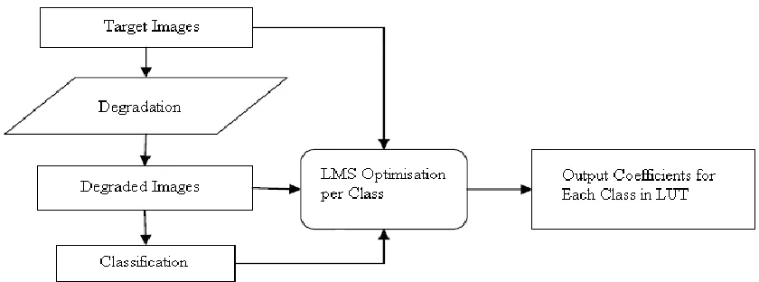
advance. Figure 1 shows the training process of the trained filters. Original images are first

degraded according to the specification of the application. The training process employs the

original video sequences and corresponding degraded video sequences as the training material

and uses the Least Squares criterion to get the optimal coefficients, which is computational

intensive due to the large number of classes. Fortunately, it needs to be performed only once.

There are various ways to degrade the original high quality sequences. Generally speaking, the

degradation during the training process is the inverse of the enhancement that one expects

during the filtering process. In this paper, two kinds of degradation methods are applied, that is

degraded images. In the degraded images, each pixel and the pixels in its vicinity are

characterized using a specific classification method. All the pixels and their neighborhoods

belonging to a specific class and their corresponding pixels in the original images are

accumulated, and the optimal coefficients are obtained by making the Mean Square Error (MSE)

minimized statistically.

Figure 1: Training process of the trained filters.

Let FD,c, FR,c be the apertures of the degraded images and the reference images for a particular

class c, respectively. Then the filtered pixel FF,c can be obtained by the desired optimal

coefficients as follows:

, , 1

( ) ( , ) n

F c c D c

i

F w i F i j







where w i i_c( ), [1... ]n are the desired coefficients, n is the number of pixels in the aperture, and

j indicates a particular aperture belonging to class c. The summed square error between the

filtered pixels and the reference pixels is:

2

2 2

, , , ,

1 1 1

( ) ( ) ( ) ( , )

Nc Nc n

R c F c R c c D c

j j i

e F F F j w i F i j

  

 

   _  _

 

where Nc represents the number of training samples belonging to class c. To minimize e2, the

first derivative of e2 to w k k_c( ), [1... ]n should be equal to zero.

2

, , ,

1 1

2 ( , ) ( ) ( ) ( , ) 0

( )

Nc n

D c R c c D c

c _{j i}

e

F k j F j w i F i j

w k  

 _  _ _

 







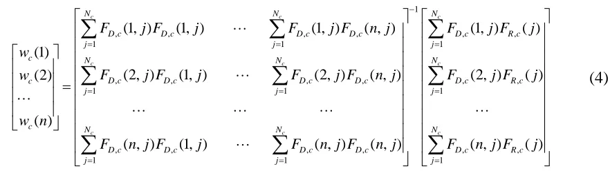
By solving the above equation using Gaussian elimination, we will get the optimal coefficients

as follows: , , , , 1 1 , , , , 1 1

(1, ) (1, ) (1, ) ( , ) (1)

(2, ) (1, ) (2, ) ( , ) (2) ( ) c c c c N N

D c D c D c D c

j j

c _{N N}

D c D c D c D c

c

j j

c

F j F j F j F n j w

F j F j F j F n j w w n          _  _{ }        









1 1 1

(1, ) ( )

(2, ) ( )

( , ) (1, ) ( , ) ( , ) ( , ) ( ) c

c

c c c

N

D c R c

j

N

D c R c

j

N N N

D c D c D c D c D c R c

j j j

F j F j

F j F j

F n j F j F n j F n j F n j F j

                          _   _              











The LS optimized coefficients for each class are then stored in a look-up table (LUT) for future

use.

Figure 2 shows the filtering process of the algorithm using the optimized coefficients. For

each pixel to be filtered, the neighboring pixels are classified in the same manner as during

training. The coefficients are retrieved from the LUT based on the classification. The pixels are

then filtered using the optimized coefficients.

2.2 Pixel Classification Methods

2.2.1 Adaptive Dynamic Range Coding Based Classification

As stated in the previous section, the momentary filter coefficients, during filtering, depend on

the local characteristics of the image, which can be classified based on the pattern of the image

region and structure information is always important for either low-pass filtering or high-pass

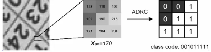
filtering. Adaptive Dynamic Range Coding (ADRC) [10] is proposed as a powerful method for

representing the structure of a region because of its high efficiency and simplicity. The ADRC

code of each pixel xi in an observation aperture is defined as: ADRC (xi) =0, if V (xi) ≤ Vav ; 1,

otherwise, where V(xi) is the value of pixel xi , and Vav is the average of all the pixel values in

the aperture. Figure 3 shows a diagram of the ADRC code on a 3x3 block.

Figure 3: The ADRC code of a 3x3 block.

2.2.2 Improved ADRC Based Classification Methods

Obviously, only using structure for classification is not sufficient, because the structure of

coding artifacts could be exactly the same as that of object details. To obtain better performance,

several additional criteria have been proposed [8]. For example, considering that high contrast

structures and low contrast structures should be treated differently, dynamic range (DR) can be

added to ADRC. DR is simply the absolute difference between the maximum and minimum

pixel values of the image region. Several other ancillary classification methods are in use, such

uniform regions. The entropy value is calculated on the probability density functions of the

pixel intensity distribution. The local entropy of a region can be defined as follows:

₂

1

( ) log ( ) N

R R

i

H P i P i



 



Where i indicates the bin index, PR (i) is the probability of pixels having a value in the range of

bin i and R is a local region inside which the entropy is calculated.

Another measure is called Mean Absolute Gradient (MAG) for determining the complexity of

a region. MAG is defined as follows:

1

1 1

(0) ( )

1

N

i

MAG F F i N





 





where F(i) denotes the intensity value of a pixel in a region, F(0) is the intensity of the pixel in

the center, and N is the number of pixels in the region. Standard Deviation (STD) is employed

as another complexity metric for a local region.

Structure information using ADRC coupled with one of the complexity measures described

above will be used for classification. For all the above complexity measures, a 13 pixel

diamond-shaped aperture, as depicted in Figure 4, is used for both classification and filtering.

Therefore, 12 bits are needed for the ADRC code, because 1 bit can be saved using

bit-inversion. And, 2 more bits are used for representing the complexity of a region. So, in total 14

bits are used for classification.

All these four complexity measures have similar behavior yet with subtle differences on

detailed regions. According to performance evaluation in [8], MAG performs the best for

sharpness enhancement and STD is the most effective for coding artifact reduction. In this

paper, the implementation of trained filters is based on the classification of ADRC plus STD,

which we consider the best for coding artifact reduction.

3. Analysis of Trained Filters

3.1 Influence of Degradation

Least squares trained filters have been successfully applied on coding artifact reduction [8, 9].

Apart from the classification method, the choice of degradation in the training process also

plays a vital role. In this section, we take a close look at the influence of different degradation

levels on the performance of the algorithm. We divide the experiment into two parts. In the first

part, we use JPEG compression to degrade the original high quality sequences to a wide range

of quality levels: from quality 10 to 90 with a step size of 10. The training set contains 25

different sequences, with a large variation of content, including natural-content-based

sequences, artificial animated sequences and some film clips, about 2000 frames in total. For

each training quality, we get a LUT. Then we apply each LUT separately to a series of test

sequences which also have a large variation of quality. Figure 5 depicts snapshots of the three

test sequences we use for our experiment. All the test sequences are excluded from the training

set. In the second part of the experiment, the main steps remain the same. Instead of JPEG

compression, we use MPEG-2 compression for degradation. Default setting is applied for

MPEG-2 except that the bit rates are ranged from 0.5M bit/s to 4M bit/s. Apparently, other

sequences. However, those new compression methods already have an in-loop de-blocker to

effectively reduce coding artifacts using coding parameters inside the encoder. The purpose of

degradation is to simulate sufficient coding artifacts which will be encountered during the

filtering process. Therefore, earlier compression standards which produce more artifacts are

preferred. Compression artifacts are not the major problem of the latest codecs like H.264/AVC

anyway.

Figure 5: Snapshot of the test sequences: Bicycle, Girlsea and Soccer.

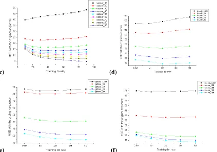
Figure 6 illustrates performance of trained filters on test sequences with different qualities

either compressed by JPEG or MPEG-2, when the LUTs are obtained by varied training

qualities.

(c) (d)

(e) (f)

Figure 6: Illustration of the influence of different training degradation levels on the output performance. (a)-(c) illustrate different training quality levels vs. MSE scores for the Bicycle, Girlsea and Soccer sequences respectively. (d)- (f) illustrate different training bit rates vs. MSE scores for the Bicycle, Girlsea and Soccer sequences respectively.

Despite minor differences in MSE behaviors, three test sequences share some common trends.

Some observations of the experiment are made as follows:

1. Test sequences with extremely good or bad quality are very sensitive to the choice of

degradation during training. For example, for the bicycle sequence compressed with

JPEG quality 10, it shows an MSE score of 70.699 when adopting the LUT trained with

severe degradation but an MSE score of 99.812 when using the LUT trained with slight

degradation. In the latter case, trained filters contribute little improvement to the test

sequence. Similarly, for the bicycle sequence compressed with JPEG quality 90, it

shows an MSE score of 3.121 when a LUT trained with slight degradation is applied

It is suggested that for high quality input, inappropriate choice of degradation level

might blur fine details and thus produce unsatisfying output.

2. Test sequences with moderate quality keep a stable output behavior when LUTs trained

with different degradation levels are used. However, we can still easily see from the

graphs that the algorithm achieves best performance when the quality of degraded

images during training is the closest to that of the test sequence.

However, in most cases, the quality of an input sequence is unknown. So it is difficult to

choose the matched LUT beforehand. As a compromise, we use a mixture of uniformly

distributed training degradation levels: from quality 10 to quality 90. As expected, it shows

better results on the average. In particular, it eliminates the most unmatched cases, which

improve the worst case performance. Let us take the Bicycle sequence as an example, the worst

MSE score is 99.812 but is improved to 79.513 if we use a mixture of degradation levels in the

training process.

3.2 Influence of Compression Methods

In this section, we explore the correlation between the type of compression methods used

during the training process and the performance of trained filters. Perceptually, we consider that

for the Soccer sequence JPEG quality 50 is comparable with MPEG-2 bit rate 1M and JPEG

quality 80 is comparable with MPEG-2 bit rate 3M. For MPEG-2, a standard implementation

with default setting is adopted. Figure 7 depicts the results on the Soccer sequence. Figure 7(a)

shows the result of training on JPEG quality 50 and applying on the Soccer sequence

compressed at different qualities by either JPEG or MPEG-2; while Figure 7(b) illustrates the

codecs at different qualities. Figures 7(c) and 7(d) are similar but trained on training sequences

compressed at higher qualities.

(a) (b)

(c) (d)

Figure 7: Illustration of the influence of JPEG or MPEG-2 compression used during the training process. (a)-(b) show the MSE scores, where the training quality for JPEG is 50 and the training bit rate for MPEG-2 is 1M bits/s respectively. (c)-(d) show the MSE scores, where the training quality for JPEG is 80 and the training bit rate for MPEG-2 is 3M bits/s respectively.

For most cases, JPEG compression shows slightly better performance. The same conclusion

can be made on other sequences. These slight differences might arise from the fact that JPEG

compression is coded without reference to other pictures in a video sequence. Each frame in

JPEG compression is treated independently. So when we set a degradation level for JPEG, the

case of MPEG, a hybrid coding scheme that uses both temporal prediction and spatial

transformation, i.e., inter- and intra-frame coding, is adopted. Three types of pictures are

defined. And only I frames are compressed with intra-frame coding, which behaves in a similar

way as the JPEG compression. But the other two types of frames, i.e. B frames and P frames,

have a less predictable quality level. For example, the B frames and P frames of two sequences

compressed with MPEG-2 using the same bit rate might differ greatly in quality. Furthermore,

MPEG-2 standard is flexible with its tolerance about the sequence combination of these three

types of frames. Thus in general, the quality of a sequence can be more easily controlled by

JPEG than by MPEG-2. As a result, JPEG compression is adopted as the degradation method

during training in the following sections.

4. Quality Adaptive Trained Filters

From the analysis in the previous section, we understand that the most optimal results can be

realized when a LUT whose degradation level during training matches with quality of the input

video frame is selected. Careless choice of LUTs might either blur details in high quality

images or preserve coding artifacts in low quality images. Thus, a quality control mechanism is

required for the trained filters. During training, several LUTs of filter coefficients are produced

by using different degradation levels. During filtering, a LUT is selected automatically for each

video frame based on its visual quality.

4.1 Block Visibility Metric

Since blocking artifact is the most annoying among all the artifacts, a block visibility metric is

adopted for measuring the visual quality of an image. This metric is a simplified version of the

discontinuities and is coherent with subjective perception, while automatically accounting for

texture masking effects in a straightforward and computationally efficient manner. Refer to [11,

12] for detailed evaluation of its coherence with subjective perception. The main idea behind

the method is that the visibility of block edges does not solely depend on the magnitude of the

gradient at the block discontinuity, but it is determined by the magnitude of the block gradient

with respect to its neighbors. In other words, block edges are visible whenever the gradient at

the edges significantly differs from the gradients in its immediate vicinity. Take the vertical

block edges as an example and the horizontal edges can be achieved in a similar way. Consider

an image I with element Iij, where i and j denote the line and pixel positions, respectively. The

absolute horizontal gradient DH can then be computed by

D i jH( , ) I i( 1, )j I i j( , ) (7) and we simply add up all horizontal gradient for each pixel to S(non-block) and when the pixel

position is a multiple of 8 we add it to S(block). Finally, the block grid visibility metric Q is

defined as the ratio of the mean accumulated value at the block edge positions and then the

mean accumulated value at the non-block edge positions:

( )

( )

S block Q

S non block



 (8)

For the three test sequences, we obtain the Q values in Table 1 when they are compressed with

different qualities or bit rates.

Input File Q Input File Q Input File Q

Bicycle_80 1.074225 Girlsea_80 1.167921 Soccer_80 1.289903 Bicycle_90 1.034740 Girlsea_90 1.085089 Soccer_90 1.151064 Bicycle_org 0.982146 Girlsea_org 0.979959 Soccer_org 1.000588

Input File Q Input File Q Input File Q

Bicycle_1M 2.216744 Girlsea_1M 2.710936 Soccer_1M 1.597243 Bicycle_2M 1.838917 Girlsea_2M 2.040262 Soccer_2M 1.325788 Bicycle_3M 1.643554 Girlsea_3M 1.693213 Soccer_3M 1.268037 Bicycle_4M 1.535949 Girlsea_4M 1.511518 Soccer_4M 1.234463

Table 1: Measurements of Q value.

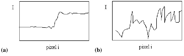
The conspicuous advantages of the block visibility metric are its mathematical simplicity and

efficiency and its coherence with visual perception. However, there is a fact that the blocking

artifacts are more annoying in flat areas, whereas they are effectively masked in textured area.

This fact is illustrated in Figure 8, which shows luminance profiles across block edges for a

relatively flat and a textured area. The gradient at block edge is identical in both scenarios.

Nevertheless, the discontinuity can be easily identified in Figure 8(a), whereas it is effectively

masked by the surrounding activity in Figure 8(b).

(a) (b)

Figure 8: Luminance profiles across a block edge for flat and textured areas.

For each sequence, Q values follow strict monotonicity. The larger the Q value, the more

severe the degradation of the sequence is. Since it is a blockiness visibility metric, Q value

varies across three test sequences, i.e. it is content-dependent. For example, for the same MPEG

compression bit rate 1Mbit/s, Q value of the Girlsea sequence arises to 2.710936 but that of the

i.e. the blockiness in the Soccer sequence has been masked by a large area of repetitive grass

content, thus gives a relatively low Q value. To make the Q value less content-dependent, we

then attempt to set up a threshold for calculation. Take the threshold of 5 as an example. If the

luminance gradient of a certain pixel is larger than 5, we just clip it and take 5 as its luminance

gradient. We also test other thresholds between 3 and 6, but there are no conspicuous

differences. This step is reasonable because some of the luminance gradient arises from the

transition in the sequence content, not because of the blockiness. And in most cases, this kind of

content transition contributes much more than the real blockiness, which is obviously

something we should avoid during calculation. Table 2 shows the Q values with clipping of the

gradient. Compared with numbers in Table 1, we can see that the Q values are less content

dependent and more stable.

Input File Q Input File Q Input File Q

Bicycle_1M 1.683782 Girlsea_1M 1.880105 Soccer_1M 1.529288 Bicycle_2M 1.373136 Girlsea_2M 1.511507 Soccer_2M 1.328376 Bicycle_3M 1.326298 Girlsea_3M 1.413591 Soccer_3M 1.293156 Bicycle_4M 1.299642 Girlsea_4M 1.353929 Soccer_4M 1.173852

Table 2: Calculated Q values with fixed threshold of 5.

Based on the above analysis, we decide to use four different levels of JPEG degradation.

These include two extreme cases: quality 10 and quality 90 degradation. When Q value of input

sequence is larger than 1.83, we use the LUT trained on quality 10 degradation. When Q value

is between 1.53 and 1.83, we adopt the LUT trained on quality 20 degradation. When Q value is

between 1.25 and 1.53, the LUT trained on quality 50 degradation is applied. The reason we use

only one LUT for this relatively large range of quality levels is that they are less sensitive to the

smaller than 1.25, the LUT trained on quality 90 degradation is utilized. These thresholds are

obtained based on extensive testing and tuning. Machine learning techniques, such as Adaboost

[9], can be also programmed to output more optimized threshold values.

4.2 Trained Filters Controlled by the Block Visibility Metric

The schematic diagrams of the training and filtering processes of the quality adaptive trained

filters are shown in Figure 9.

(a)

(b)

We evaluate our quality controlled trained filters with three other post-processing methods [2,

14, 1] for compression artifacts removal. The results of trained filters based on mixed training

using degradation levels uniformly distributed from quality 10 to quality 90 are also included

for comparison. Three more test sequences as shown in Figure 10 are used for evaluation. All

the test sequences are encoded and decoded by MPEG-2 using the default setting. Table 3

shows the resolutions and frame numbers of the test sequences. The MSE scores between

original uncompressed sequences and filtered outcomes of the compressed sequences are shown

in Table 4. The filtering is only applied on luminance and MSE scores are also only calculated

on luminance.

Figure 10: Snapshot of three more test sequences: Porschefence, Nemo and Vanessa.

Table 3: Specification of the test sequences.

Sequence Resolution Number of frames

Bicycle 720x576 200

Girlsea 720x576 50

Soccer 720x576 98

Porschefence 720x576 100

Vanessa 720x572 90

Nemo 720x480 512

Table 4: MSE scores of different methods.

Input file Quality

controlled trained filters

Trained filters - mixed

training

Ref [2] Ref [14] Ref [1]

Bicycle_2M.yuv 71.416 74.116 88.879 94.526 95.884 Bicycle_3M.yuv 50.343 51.964 68.191 69.517 70.143 Bicycle_4M.yuv 38.466 39.400 56.063 54.873 55.352 Girlsea_1M.yuv 79.115 81.674 82.621 86.656 86.634 Girlsea_2M.yuv 41.141 41.813 41.369 44.879 44.898 Girlsea_3M.yuv 21.824 22.365 22.583 24.358 24.194 Girlsea_4M.yuv 14.221 14.554 15.643 16.263 16.128 Soccer_1M.yuv 38.862 39.359 40.243 41.297 41.137 Soccer_2M.yuv 18.986 19.130 20.442 20.254 20.178 Soccer_3M.yuv 15.277 15.510 16.688 16.105 16.084 Soccer_4M.yuv 13.105 13.634 14.709 11.439 13.892 Porschefence_1M.yuv 107.429 111.974 115.505 122.428 121.984 Porschefence_2M.yuv 100.013 104.175 107.487 114.490 114.152 Porschefence_3M.yuv 54.396 54.516 60.735 62.758 62.673 Porschefence_4M.yuv 32.019 33.428 39.866 39.411 39.036 Vanessa_1M.yuv 113.048 116.749 116.314 126.095 124.230 Vanessa_2M.yuv 104.498 107.611 107.187 116.804 115.115 Vanessa_3M.yuv 62.880 63.473 65.402 71.741 71.202 Vanessa_4M.yuv 37.833 38.272 41.052 44.891 44.323 Nemo_1M.yuv 97.264 98.860 101.229 104.060 103.172 Nemo_2M.yuv 53.578 55.084 56.708 59.521 59.151 Nemo_3M.yuv 29.312 29.734 31.812 33.346 33.110 Nemo_4M.yuv 18.689 19.874 22.011 22.435 22.247

(c) (d)

(e) (f)

Figure 11: Processed results of the Bicycle sequence: (a) Unprocessed, (b) Quality adaptive trained filters, (c) Trained filters – mixed training, (d) Ref [2], (e) Ref [14], (f) Ref [1].

We can easily see from Table 3 that the proposed quality controlled trained filters yield

satisfying performance. It outperforms the three available de-blocking filters especially in some

Besides, compared with the trained filters with mixed degradation, quality controlled trained

filters always show some positive improvement.

For subjective evaluation, Figure 11 shows the results of the five algorithms on the Bicycle

sequence compressed by MPEG-2 at the bit rate of 1Mbit/s. The proposed quality adaptive

trained filters can remove various artifacts and preserve object details better than the other

methods. To show some quantitative perception related results, the Structural SIMilarity (SSIM)

[15] scores of all the test sequences are listed in Table 5. The quality controlled trained filters

outperform the three existing methods on all sequences.

Table 5: SSIM scores of different methods.

Input file Quality

controlled trained filters

Trained filters - mixed

training

Ref [2] Ref [14] Ref [1]

Bicycle_1M.yuv 0.3031 0.3035 0.3039 0.2589 0.2756 Bicycle_2M.yuv 0.3334 0.3321 0.3322 0.2785 0.2852 Bicycle_3M.yuv 0.3487 0.3467 0.3372 0.2876 0.3134 Bicycle_4M.yuv 0.3791 0.3624 0.3536 0.2907 0.3372 Girlsea_1M.yuv 0.4261 0.4251 0.4170 0.3589 0.3761 Girlsea_2M.yuv 0.4643 0.4562 0.4435 0.3701 0.3953 Girlsea_3M.yuv 0.4863 0.4777 0.4636 0.3877 0.4074 Girlsea_4M.yuv 0.4998 0.4846 0.4745 0.4035 0.4456 Soccer_1M.yuv 0.3860 0.3789 0.3698 0.3342 0.3512 Soccer_2M.yuv 0.4001 0.3991 0.3999 0.3546 0.3662 Soccer_3M.yuv 0.4153 0.4070 0.4032 0.3754 0.3824 Soccer_4M.yuv 0.4345 0.4324 0.4279 0.3908 0.3989 Porschefence_1M.yuv 0.2851 0.2789 0.2699 0.2345 0.2462 Porschefence_2M.yuv 0.2924 0.2894 0.2747 0.2563 0.2641 Porschefence_3M.yuv 0.3254 0.3119 0.3012 0.2675 0.2767 Porschefence_4M.yuv 0.3459 0.3426 0.3324 0.2990 0.2960 Vanessa_1M.yuv 0.4356 0.4292 0.4056 0.3873 0.3936 Vanessa_2M.yuv 0.4434 0.4594 0.4361 0.4091 0.4289 Vanessa_3M.yuv 0.4776 0.4636 0.4525 0.4094 0.4535 Vanessa_4M.yuv 0.4824 0.4724 0.4741 0.4207 0.4671 Nemo_1M.yuv 0.2730 0.2641 0.2679 0.2463 0.2545 Nemo_2M.yuv 0.2947 0.2790 0.2741 0.2563 0.2662 Nemo_3M.yuv 0.3253 0.3220 0.3154 0.2782 0.2873 Nemo_4M.yuv 0.3425 0.3433 0.3292 0.2943 0.3036

In this paper, we develop the classification based least square trained filters for compression

artifacts removal using the quality control mechanism. The quality metric we adopt shows

robust behavior in blockiness visibility measurement. For an input sequence with unknown

quality, the proposed algorithm can choose the most suitable LUT for filtering based on the

block visibility metric. The inclusion of the quality control mechanism coupled with the

effectiveness of the blockiness metric enables the least squares trained filters to be a decent

choice for deblocking images and videos of various qualities.

In future work, a local quality/blockiness metric will be designed to further improve the local

adaptability of the algorithm.

References

[1] L. Shao and I. Kirenko, “Coding artifact reduction based on local entropy analysis”, IEEE

Trans. Consumer Electronics, Vol. 53(2), pp. 691-696, May 2007.

[2] S. D. Kim, J. Yi, H. M. Kim and J. B. Ra, “A deblocking filter with two separate modes in

block-based video coding”, IEEE Trans. Circuits and System for Video Technology, Vol. 9,

pp.156-160, 1999.

[3] Y. Luo and R. K. Ward, “Removing the blocking artifacts of block-based DCT compressed

images”, IEEE Trans. Image Processing, Vol. 12(7), pp. 838-842, July 2003.

[4] L. Shao, I. Kirenko, A. Leitao and P. Mydlowski, “Motion-compensated Techniques for

Enhancement of Low Quality Compressed Videos”, In Proceedings of the 34th

IEEE

International Conference on Acoustics, Speech, and Signal Processing, Taibei, Taiwan, April

[5] I. Kirenko, L. Shao, R. Muijs, “Enhancement of Compressed Video Signals Using a Local

Blockiness Metric”, In Proceedings of the 33rd

IEEE International Conference on Acoustics,

Speech, and Signal Processing, Las Vegas, USA, March-April 2008.

[6] I. Kirenko and L. Shao, “Adaptive Repair of Compressed Video Signals Using Local

Objective Metrics of Blocking Artifacts”, In Proceedings of the 14th

IEEE International

Conference on Image Processing, San Antonio, Texas, USA, September 2007.

[7] T. Kondo, Y. Node, T. Fujiwara and Y. Okumura, “Picture conversion apparatus, picture

conversion method, learning apparatus and learning method”, US-patent 6,323,905, Nov. 2001.

[8] L. Shao, H. Zhang and G. de Haan, “An overview and performance evaluation of

classification based least squares trained filters”, IEEE Trans. Image Processing, Vol. 17(10),

pp. 1772-1782, October 2008.

[9] L. Shao, H. Hu and G. de Haan, “Coding Artifacts Robust Resolution Up-conversion”, In

Proceedings of the 14th IEEE International Conference on Image Processing, San Antonio,

Texas, USA, September 2007.

[10] T. Kondo and K. Kawaguchi, “Adaptive dynamic range encoding method and apparatus”,

US-patent 5,444,487, Aug. 1995.

[11] H. R. Wu and M. Yuen, “A Generalized Block-edge Impairment Metric for Video

Coding,” IEEE Signal Processing Letters, vol. 70, no. 3, pp. 247-278, Nov. 1998.

[12] R. Muijs and I. Kirenko, “A No-Reference Blocking Artifact Measure for Adaptive Video

Processing,” in Proc. 13th European Signal Processing Conference, Turkey, 2005.

[13] Y. Freund and R. E. Schapire, “A decision-theoretic generalization of on-line learning and

an application to boosting”, Journal of Computer and System Sciences, Vol. 55(1), pp. 119-139,

[14] C. Damkat, “Post-processing techniques for compression artifact removal in block coded

video and images”, Technical Report, Department of Electrical Engineering, Technische

Universiteit Eindhoven, 2004,

[15] Z. Wang, A. C. Bovik, H. R. Sheikh and E. P. Simoncelli, “Image quality assessment:

From error visibility to structural similarity”, IEEE Transactions on Image Processing, Vol.