White Rose Research Online URL for this paper:
http://eprints.whiterose.ac.uk/79281/
Version: Accepted Version
Article:
Duffy, B, Carr, HA and Möller, T (2013) Integrating isosurface statistics and histograms.
IEEE Transactions on Visualization and Computer Graphics, 19 (2). 263 - 277 (14). ISSN
1077-2626
https://doi.org/10.1109/TVCG.2012.118
[email protected] https://eprints.whiterose.ac.uk/ Reuse
Unless indicated otherwise, fulltext items are protected by copyright with all rights reserved. The copyright exception in section 29 of the Copyright, Designs and Patents Act 1988 allows the making of a single copy solely for the purpose of non-commercial research or private study within the limits of fair dealing. The publisher or other rights-holder may allow further reproduction and re-use of this version - refer to the White Rose Research Online record for this item. Where records identify the publisher as the copyright holder, users can verify any specific terms of use on the publisher’s website.
Takedown
If you consider content in White Rose Research Online to be in breach of UK law, please notify us by
Integrating Isosurface Statistics and Histograms
Brian Duffy, Hamish Carr Member, IEEE, and Torsten M ¨oller Member, IEEE,
Abstract—Many data sets are sampled on regular lattices in two, three or more dimensions, and recent work has shown that statistical
properties of these data sets must take into account the continuity of the underlying physical phenomena. However, the effects of quantization on the statistics have not yet been accounted for. This paper therefore reconciles the previous papers to the underlying mathematical theory, develops a mathematical model of quantized statistics of continuous functions, and proves convergence of geometric approximations to continuous statistics for regular sampling lattices. In addition, the computational cost of various approaches is considered, and recommendations made about when to use each type of statistic.
Index Terms—histograms, frequency distribution, integration, geometric statistics
✦
1
I
NTRODUCTIONM
ANYareas of science, engineering and medicine studycontinuous phenomena with scalar functions sampled finitely in two, three or more dimensions. Even where dis-continuous boundaries are of interest, sampling theory still assumes that the underlying phenomena and the sampling process involve functions that are continuous everywhere or nearly everywhere. Moreover, many algorithms in visualiza-tion and analysis depend heavily on computing statistics or distributions, and these have historically been based on discrete samples rather than the underlying phenomenon.
There are three reasons why statistics in visualization must account for inter-sample continuity. First, histograms are often noisy, which impedes the ability to detect features of interest, and this is directly related to the discretization of the sampling process. Second, visualization methods such as direct volume rendering depend on continuity in order to integrate optical properties. Third, multivariate data gives multi-dimensional histograms (i.e. scatterplots) with many more bins, aggravating the problems caused by discretization. Continued improvement of visualization techniques therefore depends on a solid theo-retical footing for calculating distributions from data sampled from continuous or near-continuous functions.
In this paper, we provide this theoretical footing by showing rigorously how histograms (including multi-dimensional his-tograms) measure geometric properties, and how to compute better approximations efficiently.
In practice, this starts with the recognition that statistics of sampled continuous functions are dependent on discretization in both domain and range. Range discretization (quantization) means that level sets are interval volumes (Section 5), while domain discretization (sampling) means that histograms ap-proximate quantized interval volumes (Section 5). These
ef-• B. Duffy is with the Oxford Centre for Collaborative Applied Mathematics (OCCAM) at the Mathematical Institute at the University of Oxford • H. Carr is with the Visualization & Virtual Reality Group at the School of
Computing at the University of Leeds
• T. M¨oller is with the Graphics, Usability, and Visualization (GrUVi) Lab at the School of Computing Science at Simon Fraser University
fects can be dealt with by applying Geometric Measure Theory to integrate over the quantized interval volumes (Section 4). The principal contributions of this paper are thus:
1) We show the importance of understanding Lebesgue integration and Federer’s Co-Area formula in relation to quantized data. However, while Lebesgue integration is necessary to understand the mathematical foundations of histograms, Riemann integration suffices for our proofs (Section 4).
2) We introduce the necessary correction for quantized statistics and demonstrate they are in fact volume statis-tics computed by Riemann integration (Section 6). 3) We provide a formal proof of convergence for quantized
statistics and geometric properties based on Riemann integration (Section 6).
We contribute further by splitting scalar field statistics into two groups, volume statistics (Sections 5 and 6) and surface statistics (Section 7). We then show the difference between these (Section 9) and summarise which statistic to use (Section 11) based on computational performance (Section 10).
We therefore start by reviewing previous work (Section 2) and the mathematical notation (Section 3) necessary for Federer’s Co-Area formula (Section 4). Supplementary mate-rials relating to Section 4 are in Appendix I and II. Finally, Appendix III gives a detailed account of all data sets and implicit functions used for evaluation throughout this work.
2
R
ELATEDW
ORKAt the heart of this work is the relationship between histograms and other distribution statistics, geometric properties of iso-contours, considerations of algorithmic efficiency, and measure theory. We will discuss measure theory in the next section and review work in visualization on statistics, geometric properties, and algorithmic efficiency in this section.
extracted, corresponding to statistically significant features. Other statistical moments, such as variance and standard deviation, skewness and kurtosis proposed by Tenginakai et al. [1], [2], have also been used to detect salient features.
Histograms are used in transfer function design [3] to assign optical properties to isovalues. Multidimensional histograms have been used by Kindlmann et al. [4], [5], [6] and by Kniss et al. [7], [8] to exploit relationships between isovalues and gradients. In a further variation, local histograms were proposed by Lundstr¨om et al. [9] to allow users to examine sub-regions of the volume in greater detail.
Geometric properties of isosurfaces were introduced by Bajaj et al. [10], [11] instead of histograms in visual interfaces. Algorithmically, Shen, Hanson & Livnat [12] used the range of isovalues in each cell (the span) in data structures to accelerate isosurface extraction. Similarly, Fujishiro & Takeshima [13] extended a measure of spatial coherence from grey-scale images in 2D to volumetric data in 3D, using the difference between adjacent samples to measure coherence, and one of the principal purposes of this work was to improve the algorithmic performance of visualization techniques.
Carr et al. [14] identified the fundamental relationships between statistics, geometry and algorithmic performance, introduced continuity, and argued that algorithmic properties such as active cell count could substitute for histograms.
Scheidegger et al. [15] corrected errors in detail of this work and showed that geometric surface statistics do not measure the same properties as the histogram. They adjusted the geometric surface statistics via Federer’s Co-Area formula to account for gradient changes over the scalar field, approximating the gradi-ent with the span of the isosurfacing cells. Although based on geometric measure theory, this work approximated measures with discrete computations and overlooked the existence and contribution of cells with no span (i.e. zero gradient).
Bachthaler& Weiskopf [16] extended the continuous models to multidimensional histograms, markedly improving scatter-plots for meshes representing continuous phenomena.
In summary, work in this area has unified the roles of statistics, geometry, algorithmic performance and measure theory, but left several elements unresolved: quantization in the range, the impact of cells with zero span or gradient, and whether algorithmic approximations can be guaranteed to give the same answer as the histograms. We therefore first develop some notation and summarize the relevant mathematics.
3
D
EFINITIONS& N
OTATIONSince the proofs that follow use formal definitions of inte-gration, we state the relevant terms here, referring readers to Federer [17] or Morgan [18] for further information. We shall stick as strictly as possible to Federer’s notation, although there are respects in which it could be simplified.
We also note that the geometric measure theory is not restricted to functions with one-dimensional domains and ranges, but applies more generally to functions with arbitrary dimensionality. We therefore start by assuming that we have a function f : A⊂X =IRm→B⊂Y =IRn from a subset A in the domain X =IRm to a subset B in the range Y=IRn.
Range
Domain
A
B
F
IR
mIR
nIR
m+n
y
Embedding Space E = Y =
X =
(f−1)
E(y)
(f−1)
[image:3.612.313.561.54.205.2]X(y)
Fig. 1: Here we show the relationship between the domain X =IRm, the range Y =IRn, and the embedding space E= IRm+n. Note how the inverse image f−1(y)can exist either as a subset(f−1)E(y)of F⊂E or a subset(f−1)X(y)of A⊂X .
For convenience, we shall assume that A is of size 1 - more precisely, of m-dimensional Hausdorff measure 1 (see below).
Lipschitz Function: As defined in Federer [17], Lipschitz
functions generalize the idea of functions of limited gradient - i.e. continuous functions. Thus, a function f : X →Y is a Lipschitz function from a metric space X to another metric space Y iff∀a,b∈A there is some finite number K such that:
dY(f(a),f(b))≤KdX(a,b) (1)
where dX and dY are the metrics for X and Y respectively. Although this definition applies to a variety of metric spaces, we are primarily interested in Euclidean spaces, and will therefore assume that dX and dY are Euclidean metrics and that the function f is Lipschitz.
Functions as Manifolds: For a Lipschitz function f :
A⊂X →B⊂Y , we can think of f as defining a set F =
{(x1, . . . ,xm,y1, . . . ,yn)∈E :(x1, . . . ,xm)∈A,f(x1, . . . ,xm) =
(y1, . . . ,yn)∈B}. Since f is Lipschitz, F will be an m-manifold
embedded in the m+n-dimensional space constructed by
E =IRm×IRn, the direct sum of the spaces X =IRm and Y =IRn. For convenience, we will refer to this space as the embedding space E of X and Y . Where m=2 and n=1, then X=IR2is the infinite plane shown in Figure 1, A is a region on the plane, and f : A→B is a height function defined on A, where B⊂IR is the range of height values taken on by f . Moreover, the embedding space E=A×B⊂IR2×IR1=IR3 is a three-dimensional space in which the function defines a terrain, and F is the terrain itself, embedded in E.
Riemann Integration: In real analysis, Riemann integration
is the most commonly used form. To approximate area under a curve, the x-axis (the domain) is divided into segments. Rectangles are constructed on each segment to fit under (or over) the curve, and the area approximated as the sum of the areas of the rectangles. As the segment length approaches zero, the sum approaches the area under the curve: from below if rectangles are fitted under the curve, the lower bound, from above if rectangles are fitted over the curve, the upper bound. This approach to integration uses Euclidean cross products between segments in the domain and range of the function to construct measuring patches, i.e. for f : IR1→IR1 the
corresponding patch is of dimension IR1×IR1=IR2, a
rectan-gle. Higher dimensional integration can be performed using the same principles by taking rectangular segments in the domain and range, where a rectangle is understood to mean a Euclidean cross product of arbitrary dimensions.
For dimensional domains and n-dimensional ranges, m-dimensional patches are used instead of segments, and m+ n-dimensional regions instead of rectangles. We write:
Z
A
f(x)dmx (2)
where the exponent m can be added when integrating over more than one dimension. While sufficient for most problems, Riemann integration breaks down for certain functions that are well-behaved in the range but not in the domain.
Squeeze Theorem: For a given function f(x), convergence is shown by trapping f(x)between upper and lower bounding Riemann integrable functions g(x)≤ f(x)≤h(x) for all x in an open interval containing a, except possibly x=a. If limx→ag(x) = limx→ah(x) =L, then the Squeeze Theorem forces limx→af(x) =L, and similarly for left and right limits. We note that this is a sufficient condition for convergence of Riemann integrals: as we are using it to prove our result, we do not require it to be a necessary condition.
Lebesgue Measure: To remedy the flaws in Riemann
integration, Lebesgue stepped back from integrating functions, and started with the simpler problem of measuring the size of the set B. Instead of a limit as patch size approached zero, Lebesgue used Borel sets: collections of subsets of A which are closed under countable union or intersection. Provided that a Borel set covers the set of interest, the Lebesgue measure
L(A) of A replaces the concept of the limit by taking the minimum sum of sizes of Borel sets that covers A.
Lebesgue Integration: To integrate a Lipschitz function
f(x)over A, Lebesgue integration computes the minimal sum of sizes of the Borel elements multiplied by the value of f(x) at the centre of the Borel element. When Lebesgue integration is explicitly intended, it is written as:
Z
A
f(x)dLmx (3)
Lebesgue measures and integration are a key aspect of geo-metric measure theory and are discussed in Section 4.1.
Hausdorff Measure: In general topology, sets are covered
with open balls (abstractions of circles / spheres). With a sim-ilar definition to Lebesgue measures, the Hausdorff measure of an object H(A) is the sum of the sizes of the minimal
Range
Domain A
B
F
IRm
IRn IR
m+n Embedding Space E =
i
Q
(fQ−1)E(i)
[image:4.612.315.531.53.190.2]Ai= (fQ−1)X(i)
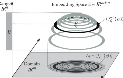
Fig. 2: Here we quantize the same function f as in Figure 1 to a function fQ. In fQ, only quantized values i∈B have non-empty inverse images. Quantization thus replaces the manifold F with a piecewise manifold FQwhose pieces are the inverse images (fQ−1)E(i). In the domain, the corresponding inverse images become interval regions Ai= (fQ−1)X(i) defined by isocontours at i+0.5 and i−0.5 of the non-quantized function.
open-ball covering of A. The Hausdorff measure is usually considered the best measure of object size, as it matches more general topological expectations. For a set of dimension
m embedded in a space of dimension m+n, the Hausdorff
measure is always m-dimensional, as it measures the intrinsic size of the set. Since we will end up with different spaces in which sets can be measured, we will make explicit the
space in which we measure by writing Hm
X to indicate the m-dimensional Hausdorff measure in the space X .
Hausdorff Integration: We can also integrate with respect
to Hausdorff measures. The process is similar to Lebesgue integration, using open balls instead of boxes, and is written:
Z
A
f(x)dHm
X x (4)
where the subscript indicates the space in which we measure.
Besicovich Covering Theorem: To link the Hausdorff
measure to the Lebesgue measure, the Besicovich covering theorem states that measures based on patch shapes other than open balls converge provided that there is a constant ratio between the patch size and open balls.
Jacobian: A generalized version of gradient, the Jacobian
is the corrective factor that relates elements of regions of the domain of a function to images of the function. For f : IRm→ IRn, differentiable at x, the Jacobian is based on the m×n differential matrix D f of the partial derivatives of each of the n output variables with respect to the m input variables.
The k-dimensional Jacobian of f , written Jkf(x), is the maximum k-dimensional volume of the image under D f of a unit k-dimensional cube as described by Morgan [18]. If rankD f(x)≤k, then(Jkf(x))2is the sum of the squares of the determinants of the k×k submatrices of D f as per Morgan1. Conveniently, where n=1 (i.e. f is a scalar field), the Jacobian matrix is simply an m×1 vector, and the Jacobian is the magnitude of the gradient of f , i.e. J1f(x) =k∇f(x)k. If
m=n=1, f is a curve embedded in two dimensions, and the
slope of the tangent line is the Jacobian. For arbitrary m and n, the Jacobian measures distortion from the domain A to the manifold F. For clarity, Appendix I shows a worked example.
Sampling (Discretization in the Domain): We assume
that the continuous function f : A→B has been sampled at a discrete set of N distinct points PN on a regular lattice. Since a regular lattice is defined by a set of m independent vectors~vj∈X=IRm,j=1. . .m, each sample point p can be written as the weighted sum of integer multiples of the vectors, p=∑mj=1wj~vj: wj∈Z. The set PZ N of sampling points is then all distinct sample points pi in the domain A:
PN={p= m
∑
j=1wj~vj: wj∈ZZ,p∈A} (5)
where N is determined by the number of points on the lattice within the domain A. As we will see in Section 5.3, a set of patches covering the domain is induced by the Voronoi cells of the sampling points in PN. As N increases, these patches can then be used for Riemann integration.
Quantization (Discretization in the Range): In addition
to quantizing in the domain by means of sampling, machine representations of data quantize in the range: even floating point values are quantized at the level of machine epsilon. For a scalar field f : X →IR, the effect of this is to divide the domain into a set of disjoint regions with distinct values. In 2D, where a scalar field can be represented as a terrain in 3D, quantization results in a new function fQthat takes the form of a set of terraces, as shown in Figure 2. Where quantization is combined with sampling, these terraces then get approximated by sets of prismatic columns perpendicular to the domain.
Level Set Measure: Given any function f , the level set
measure πf measures the size of the level set for each given value y∈Y . For any value of y, πf(y)is thus the Hausdorff measure of the inverse image f−1(y).
πf(y) =Hm−n(f−1(y)) (6)
Histogram: For a discrete set of quantized samples, the
histogram is the proportion of the samples with a given value. The histogram samples are at the centers of Voronoi cells. We assume that the total volume of the domain is 1 and the size of a Voronoi cell K is size(K) =1/N (see the discussion of boundary conditions below), as there are N rectilinear Voronoi cells in each lattice, one for each sample. We therefore define the histogram over N samples to be:
HN(i) =
∑
f(p)=i,p∈PN
size(K) (7)
Voronoi Cells: As previously shown [14], histograms
com-puted for a sampling involve the Voronoi cells of the samples. For each point p∈PN, its Voronoi cell is the set of points that are closer to p than to any other sample:
Vor(p) ={q∈A : d(q,p)<d(q,p′)∀p′∈PN\ {p}} (8)
Figure 3 shows samples on a square lattice in two dimensions as dots, and their Voronoi cells as squares. Since a regular lattice uses integer-weighted sums of the basis vectors, all Voronoi cells except those at the boundaries will be home-omorphic and have the same Hausdorff measure. It is then
easy to see that Nearest Neighbour interpolation reconstructs f by assigning the value f(p)to each point q∈Vor(p).
Delaunay Cells: Our approximations using geometric
prop-erties are not calculated with the Voronoi cells. Instead, as in Marching Cubes and related algorithms, we calculate geometric properties using the Delaunay cells Del(PN)of the point set PN. Formally, the Delaunay complex Del(PN)is the set of cells which satisfies the condition that no point in PN is in the interior of any closed ball circumscribing any cell in Del(PN). A point set PN in X=IRm is said to be degenerate if there is any set of m+2 or more points from PN on the boundary of any closed ball that contains no other vertices. If the point set is not degenerate, then all cells in Del(PN)must be simplices (triangles in 2D, tetrahedra in 3D).
Where PN is degenerate, however, cells may be arbitrary convex polyhedra. For Cartesian sampling lattices, the Delau-nay cells are m-cubes with sample points as vertices: i.e. the Delaunay cells are the cells used by marching algorithms.
Boundary Conditions: Voronoi cells at the boundary of the
domain may not actually be homeomorphic. We avoid this by offsetting the samples by half a lattice unit, i.e. by assuming that a point sample occurs at the centre of the pixel rather than the corner. The Delaunay cells of these samples are then non-uniform, as half- and quarter- pixels occur at the boundary. To keep our computations consistent, we therefore make the simplifying assumption that the function is periodic across all boundaries, resulting in N Delaunay cells of size 1/N each.
4
F
EDERER’
SC
O-A
REAF
ORMULAWe now turn to one of the major results in geometric measure theory - Federer’s Co-Area Formula [17]. However, the use of this work in computational statistics and visualization has var-ied significantly in notation, making the relationship between published papers unclear. Moreover, there is a significant flaw in how this theorem has been applied. We therefore develop the required results directly from Federer’s Co-Area Formula, and use Appendix II to reconcile the notation in previous work.
4.1 Lebesgue Measures in Domain and Range
As stated above, Lebesgue integration is often used to integrate over the range of a function rather than the domain. This can be used in several ways, but the simplest is that any integral is merely the Hausdorff measure of a particular set. For example, for f(x): IR→IR, we can measure the areaRb
a f(x)dx between the curve and the x-axis, or we can measure the size of F: the arclength of a segment of f plotted in two dimensions.
For the purposes of this paper, we are primarily interested in the measure of F - but as we will see shortly, Lebesgue integration can readily be extended to other integrals. To see how various measures relate, we return to Figure 1.
Since f is a manifold F in the embedding space E, it is natural to measure A, B, or F, and to ask how these measures are related. To get the measure of A, we take:
Hm X (A) =
Z
A
For the measure of F, we start with Federer’s Area Formula 3.2.3 [17], where for a Lipschitzian function f : IRm→IRm+n with m≤n and anLm measurable set A:
Z
A
Jmf(x)dLmx= Z
IRnN(f|A,y)d
H my (10)
Morgan [18] points out that if f is a smooth embedding, then the right hand side of Equation 10 is the Hausdorff measure of f(A), i.e. the left-hand side of Equation 9. Before proceeding, we observe that Federer uses f , g, m and n to refer to different things here and in the Co-Area formula. We therefore regularize the notation by defining a mapping function g : IRm→IRm+n: g(x) = (x1, . . . ,xm,f1(x), . . . ,fn(x))
which parameterizes the manifold F from the region A in the domain. Since g is Lipschitzian with m≤m+n, it satisfies the requirements for Equation 10, and we can compute the Hausdorff measure of F:
Hm E (F) =
Z
A
Jmg(x)dLmx (11)
using the Jacobian Jmg(x) to correct for the projection. We give a small example in Appendix I to clarify the notation and the relationship between the Area and Co-Area Formulas. It is also possible to compute measures of f−1(y)in A or in E: since y is fixed, fE−1is restricted to a subspace of E parallel to the domain X , as shown in Figure 1. The Hausdorff measure of f−1(y)must then be identical in X and E:
πf(y) = HXm−n((f−
1)X(y))
= Hm−n
E ((f−1)E(y))
= Z
(f−1)
E(y)∩F
1dHm−n
E x (12)
4.2 Federer’s Co-Area Formula
For cases where Riemann integration breaks down, integration can often be done over the range Y =IRn rather than the domain X=IRm. If f is invertible, this is trivial, but if not, a different approach is instead needed.
In general, f is non-invertible: f−1(y)is a set of dimension m−n rather than a point. However, f−1(y)can be measured for each y, and the Co-Area formula integrates over y∈Y rather than over x∈X . Thus, for a givenLm measurable set A in the domain of a Lipschitz function f : X=IRm→Y=IRn where m>n, Federer’s Co-Area formula (3.2.11) states that:
Z
A
Jnf(x)dLmx= Z
B
Hm−n(A∩f−1(y))dLny (13)
Adding subscripts to show the integrating space, we get:
Z
A
Jnf(x)dLmx= Z
B Hm−n
A (A∩(f−1)A(y))dLny (14)
In other words, we can integrate over the projection of F into the domain X=IRm or the projection of F into the range Y=IRn. In either case, the integration computes the measure of patches in the projection, then multiplies those measures by a perpendicular measure estimating spatial distortion. For Riemann integration, the patches are a set of disjoint patches that sum up to either A or B, while Lebesgue integration takes the minimum sum over all Borel covers of either A or B.
Although it might seem that this equation computes the Hausdorff measure of F, the Jacobian Jnf(x) used in this equation is not the same as that used in Equation 11. We provide a small example in Appendix I to clarify this issue.
Moreover, Equation 14 is primarily about measuring a region, rather than integrating a function over that region. This task of integration is done by introducing a new function in Federer’s Theorem 3.2.12. In this, we take anyLmintegrable IR valued function g : X=IRm→IR (where IR is the extended reals IR∪ {−∞} ∪ {∞}). Then,
Z
A
g(x)Jnf(x)dLmx= Z
B Z
f−1(y)g(x)d
Hm−nxdLny (15)
and, with subscripts indicating the integrating space:
Z
A
g(x)Jnf(x)dLmx= Z
B Z
(f−1)
E(y)
g(x)dHm−n
E xdLny (16)
This implies several things about the use of Federer’s Co-Area formula for scalar and multivariate fields and applica-tions. We defer this discussion to Appendix II, along with the relationship between Riemann and Lebesgue integration and reconciliation of Federer’s notation with that used in the related work. At this stage, we can make the following observations:
1) Although Lebesgue integration is more general than Riemann integration, many practical problems are solved with Riemann integration for the sake of simplicity. 2) Lebesgue integration was introduced in part to deal with
functions that were well-behaved in the range but not in the domain. In the case of functions quantized for machine computation, we actually have functions that are well-behaved in the domain but not in the range. 3) Although Federer’s Co-Area Formula uses
Lebesgue-integrable functions, all of our data sets in practice are sampled at finitely many locations - our reconstructed function is therefore always Riemann-integrable. 4) For the geometric approximations of distributions
intro-duced by Carr et al. [14], convergence is easier to prove with the mechanics of Riemann integration.
For the above reasons we will prove convergence using Riemann integration rather than Lebesgue integration.
5
C
ONVERGENCE OFH
ISTOGRAMSHaving understood the Co-Area Formula, we turn our attention to the histogram, and in particular, to demonstrating that the histograms of a quantized function represent volume statistics. Specifically, histograms fundamentally represent the measure of an interval volume defined by quantization.
5.1 Quantization and Interval Volumes
and i+0.5. The inverse image of any integer i∈B is then the region Ai= fQ−X1(i)⊂A in the domain that is bounded by these two isocontours. It then follows for scalar fields in three dimensions (m=3,n=1) that these regions are interval volumes, as described by Guo [19] and Fujishiro et al. [20].
5.2 Measuring the Interval Volumes
We now observe that fQ−1(y)is an interval volume of dimen-sion m iff y∈B is an integer i, and of dimension 0 otherwise. It then follows that Equation 6 cannot be applied to compute an (m−n)-dimensional Hausdorff measure for πfQ, and that
fQ is discontinuous and thus not Lipschitz.
However, we can remedy this problem if we observe that each Ai is a bounded subset of the domain X , and that f is (still) a Lipschitz function. Applying Equation 15 to Ai, we can computeπfQ in terms of f as follows:
πfQ(i) = H
m(Ai)
= Z
Ai
1dLmx
= Z
Y Z
(f−1)
E(y)∩Ai
1 k∇fkdH
m−n
E xdL
ny
=
Z i+0.5
i−0.5
Z
(f−1)
E(y)
1 k∇fkdH
m−n
E xdL
ny (17)
Interestingly, in this form, the Jacobian is retained, and it becomes clear why the formulation in Scheidegger et al. [15] performs as desired: the Jacobian term is required for the Lebesgue integration, which is performed over an interval of size 1. Similarly, Bachthaler & Weiskopf’s mass density [16] formulation already includes the Jacobian in their definition ofσ(ξ). We note that they render to an image, thus implicitly quantizing the result to bins of fixed size δy. In effect, therefore, their model performs a Riemann sum with regions of size δy, and produces the same result as the histogram.
Moreover, a corollary of this is that the sum ofπfQ over all
integer i∈Y must be the total volume of the domain A:
Vol(A) =
∑
i∈YπfQ(i) (18)
Before covering the implications of this, we first show that the histogram converges to πfQ as sampling resolution increases.
5.3 Histogram Convergence
We take our definition of the histogram HN, and assume that the samples are on a square lattice as in Figure 3. From Section 3, we know that the Voronoi cells in a regular square lattice are all of Hausdorff measure size(K) =1/N. We claim the limit of the histogram HN tends toπfQ as N tends to infinity:
lim
N→∞HN(i) =πfQ(i) (19)
We have assumed in Section 3 that f is Riemann integrable. We therefore measure the size of the region bounded by the two contours at i+0.5 and i−0.5 using Riemann integration over the Voronoi cells of the samples, as shown in Figure 3. As the patch size approaches zero, the area computed will then converge to the correct answer in the limit. In general,
j-0.5
j+0.5 j
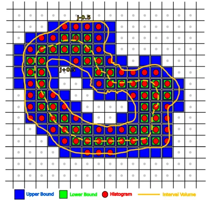
[image:7.612.332.538.47.247.2]Upper Bound Lower Bound Histogram Interval Volume
Fig. 3: The Voronoi cells of sample points can be used to prove convergence of the histogram HN toπfQ as N→∞.
the patches need not be of uniform size, but our proofs assume a regular lattice, so all patches will be of uniform size(K).
To demonstrate that the histogram converges to the measure of the interval region, we define an upper bound UN(i)and a lower bound LN(i)which are known to converge correctly by the Squeeze Theorem, and show that the histogram HN(i) is trapped between these bounds. For our lower bound LN(i), we count the set of Voronoi cells strictly contained in the interval region, as shown by green squares in Figure 3, and multiply by size(K). As LN(i) is contained inside the interval region it must converge because the interval region converges. LN(i) is analogous to the lower Riemann sum of a 1D function. Similarly, for our upper bound UN(i), we choose the set of Voronoi cells intersecting the interval region, as shown as blue squares in Figure 3. As UN(i)is the total cover of the interval region it must also converge. UN(i)is analogous to the upper Riemann sum of a 1D function. By Riemann integration, these bounds converge as N increases and size(K)decreases:
lim
N→∞LN(i) =πfQ(i) =Nlim→∞UN(i) (20)
Now, as shown by red circles in Figure 3, the histogram counts all samples whose values quantize to i, i.e. all samples in the interval region Ai. We claim that HN(i)≥LN(i)for all N. First, every Voronoi cell in Figure 3 which is counted for LN(i)is entirely contained in Ai, and therefore the sample that defines it must be in Ai, i.e. the sample quantizes to i. It then follows that the samples corresponding to these Voronoi cells are a subset of the samples counted by the histogram, and the inequality holds. By a similar argument, HN(i)≤UN(i), i.e.:
LN(i)≤HN(i)≤UN(i) (21)
Then, as the Voronoi cell size(K) approaches zero, the his-togram is trapped between two converging sequences, and must also converge toπfQ(i), as in Equation 19.
6
G
EOMETRICV
OLUMES
TATISTICS(a) 32× 32 (b) 128× 128
Fig. 4: In (a) and (b), a spherical distance field was sampled and quantized to the range [0-20]. Cells containing isocontour j=11 are marked in green. Cells marked red are homogeneous cells, introduced by quantization, where all values equal j.
geometric approximations of volume statistics converge to the same result. However, in constructing the proof, it becomes apparent that the formulas reported by Carr et al. [14] and Scheidegger et al. [15] need correction, as they do not handle all of the consequences of quantization correctly.
Scheidegger et al. [15] approximated contour size by inverse gradient weighting either the area of triangulated isosurfaces or the number of active cells for any given isovalue, then approximated gradient magnitude with the span of the cell. While the result converged empirically, there is a subtle effect that is evident in particular for active cell count statistics.
We observe that contours are typically extracted using marching algorithms that divide the space into a mesh whose vertices are sample points, then extracted separately in each cell of the mesh. Carr et al. [14] showed that for a regular lattice of sample points, the appropriate mesh is the Delaunay complex of the samples, instead of the Voronoi complex.
For a given isovalue i, the values at a cell’s vertices are compared to i and classified as black if their value is>i, white if≤i. A surface is constructed in the cell iff some vertices are black and others white. Now consider a cubic Delaunay cell K, all of whose vertices have isovalue h. For all isovalues<h, all vertices are classified black, so no contour is drawn, while for isovalues>h, all vertices are classified white, and no contour is drawn. Under trilinear interpolation, however, every point x in the cell has function value f(x) =h. Correspondingly, the inverse image f−1(h) =K is a volume, not a surface. In
practice, this is avoided by classifying vertices as white if they are ≤i, so no surface at all is extracted.
We refer to cells whose vertices share an isovalue as homogeneous cells. Since the span of such a cell is zero, using it to approximate inverse gradient magnitude would cause an exception. But contouring algorithms treat homogeneous cells as inactive for all isovalues, so no surface is extracted, and
TABLE 1: Empirical results from the 94 8-bit and 23 12-bit data sets used by Carr et al. [14] show a large percentage of zero spans. For the 12-bit data sets, with more quantization levels, the proportion of zero spans unsurprisingly decreases.
Type All Medical Measured Synthetic
8-bit 31.40% 25.70% 44.10% 25.20%
12-bit 8.98% 5.57% 14.72% 4.63%
no statistic exists to be inverse gradient-weighted. As a result, Carr et al. [14] and Scheidegger et al. [15] do not process homogeneous cells, and therefore do not include them in the overall statistics - contrary to Equation 18.
6.1 Evidence of Homogeneous Cells
The existence of homogeneous cells may seem a quibble. In quantized data, however, they are surprisingly common, and affect the accuracy of geometric statistics. Before proceeding, we therefore confirm their existence in implicit functions and in real-world data. A more detailed account of these data sets can be found in Appendix III. We illustrate this in Figure 4, using a circular distance field over the domain IR2constrained to the sampling window x= [−1,+1] and y= [−1,+1]. The results of this are shown in Figure 4 for the range[0,20]. As cell size decreases, a smaller proportion intersects the contour at isovalue j=11 (shown in green), and homogeneous cells appear between active cells, as shown in red.
[image:8.612.73.543.51.298.2]In practice, floating point data is re-quantized to lower precision to compute histograms of scalar fields. For this reason we restrict ourselves to the typical quantization levels 8, 10 or 12 bit. We note that for floating point data homogeneous cells will occur with much lower frequency.
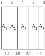
1 2 3 4 5
1.5 2.5 3.5 4.5
[image:9.612.336.539.47.245.2]A2 A3 A4A5 A1
Fig. 5: Interval regions Ai intersecting a single cell K. The isovalue range in the cell is from 1.0 to 5.0, and we accordingly divide it into slabs for which f rounds off to integer values. Given linear interpolation, the slabs A1 and A5 are then half
the width of the remaining slabs, as half of the ranges that round off to 1 and 5 are outside the cell.
We also observe that the volumetric coherence introduced by Fujishiro & Takeshima [13] relates to the homogeneous cells. These cells have zero span, and must necessarily have the same isovalue at all of the vertices. Since this implies that there are samples at isovalue i adjacent to other samples at isovalue i, homogeneous cells occur along the main diagonal of the co-occurence matrix Pδ, but are excluded from the volumetric coherence VCM by a term(i−i). Since low values of VCM are taken to mean highly coherent volumes which can be rendered efficiently, the connection between statistics, geometry and algorithmic performance can again be seen.
6.2 The Histogram & Geometric Statistics
We now know that histograms approximate measures of inter-val volumes, and previous computations based on continuous formulas combined with discrete extraction using Marching Cubes do not correctly account for the entire domain. We will see in Section 9 the practical implications of this. First, however, we modify the formulas explicitly to account for the entire domain, and prove convergence to the correct result.
We observe that an interval region Ai includes isovalues in the range[i−0.5,i+0.5). From Section 3, we assume that the Delaunay cells wrap around, and that size(K) =Vol(A)/N.
The span of a cell K is span(K) =max(K)−min(K), and K intersects span(K) +1 interval regions Ai, as shown in Figure 5, where span(K) =5−1=4, but there are 5 interval regions A1, . . . ,A5 intersecting the cell. Of these, A1 covers isovalues
in the range[1.0,1.5)– i.e. the range is half as great as for A2,
so we give A1and A5(i.e. Aminand Amax) half as much size as
the remaining regions. This is precise for linear interpolation, but not for other interpolants.
j-0.5
j+0.5 j
Upper Bound Lower Bound Cell Inter. Interval Volume
Fig. 6: For our approximations DN(i)and CN(i), the Delaunay cells of the sample points are used to prove convergence to
πfQ as N→∞.
This leads to the following approximation ofπfQ:
DN(i) =
∑
K∈Del(PN)
size(K)di(K) (22)
di(K) =
0, AiTK=/0
1, AiTK6=/0,span(K) =0
1
2span(K), AiTK6=/0,i=min(K)
1
2span(K), AiTK6=/0,i=max(K)
1
span(K), otherwise
(23)
where Del(PN) is the Delaunay complex of PN and min(K) and max(K)are the extremal values of the cell.
In this formulation, Delaunay cells entirely outside the interval region Ai contribute 0, those entirely inside (i.e. homogeneous cells) contribute 1, and other cells contribute a proportion of the cell based on 1/span(K) as shown in Figure 5. We note that the result of this is that each cell K is guaranteed to contribute 1 to the overall computation, thus preserving the measure of A as the sum of the measures of Ai:
Vol(A) =
∑
i∈YDN(i) (24)
as required by Equation 18. We claim that the limit of DN must tend toπfQ as N tends to infinity:
lim
[image:9.612.136.212.135.230.2]N→∞DN(i) =πfQ(i) (25)
Figure 6 shows the proof: note the parallel with the proof for the histogram, except here the integration patches are Delaunay cells instead of Voronoi cells. Delaunay cells wholly in the interval region Ai, i.e. with span zero, form the lower boundLN(i)of the squeeze, while the cells that intersect the
interval region Ai form the upper bound UN(i). DN is then trapped betweenLN andUN as shown in Figure 6 by shading
the fraction of the cell attributed to DN(i)by Equation 23.
LN(i)≤DN(i)≤UN(i) (26)
[image:9.612.328.564.308.413.2]6.3 Weighted Area Convergence
As discussed in the previous work [14], [15], it is also possible to approximate the distribution function by taking the area of the isosurface for each cell and multiplying it by the inverse gradient magnitude or cell span. In effect, this replaces the isosurface with a thin shell of non-uniform thickness, that measures the volume (i.e. region size) of this shell.
This approximation also needs to be adjusted to include homogeneous cells, and proven to converge to Equation 17. As it is based on the size of the interval region Aisurrounding the contour at isovalue i, we use CN(i):
CN(i) =
∑
K∈Del(PN)
ci(K) (27)
ci(K) =
0, AiTK=/0
size(K) AiTK6=/0,
span(K) =0 Z(K,i−0.5)
2
t
span(K) AiTK6=/0, i=max(K) Z(K,i+0.5)
2
t
span(K) AiTK6=/0, i=min(K) Z(K,i−0.5)+Z(K,i+0.5)
2
t
span(K) otherwise (28)
Here, Z(K,x) is the Hausdorff measure of the contour of f at isovalue x in cell K, approximated by marching cells. t = (size(K))1/m is a term that approximates the thickness of the cell with its linear dimension. The effect of this is to compute an approximation of the portion of KTf−1
Q (i). Unlike Equation 23, however, the sum of these terms is not guaranteed to sum to 1.
As with DN(i)the proof utilizes the squeeze principle, based on the recognition that we are computing region size. However, rather than treating the inverse gradient magnitude term as a fraction of the cell, we now treat it as the thickness of a shell. We again use homogeneous cells in Ai for the lower bound LN(i). We then define an upper bound for some constant k:
Uk
N(i) =LN(i) +k(UN(i)−LN(i)) (29)
We know that, in general, for any fixed k, f and f+g converge iff f and f+kg converge. Since we have shown that UN(i) and LN(i) converge to Equation 17. We therefore conclude thatUk
N(i)will also converge to Equation 17 for any fixed k. We use this conservative upper bound to simplify the proof.
As before, it is easy to see thatLN(i)counts exactly those homogeneous cells captured by the second branch of Equation 28, and it follows that LN(i)≤CN(i). Now, to construct our upper boundUk
N(i), we start by observing that DN(i)counted the size not only of the homogeneous cells, but also some fraction of the size of all cells on the boundary. Note that this fraction was an approximation of the portion of the cell covered by the interval region, and was computed by assuming that all interval regions intersecting the cell were the same size. In the present instance, instead of arbitrarily dividing the cell into regions of equal size, we wish to approximate the size of the region by taking the inverse gradient as an estimate of the
thickness of the interval region, and multiplying by an estimate of the other dimensions of the interval region: in this case an estimate of the length of the contour. It is not immediately clear that this approximated region will lie entirely inside the cell, and our convergence proof must adapt to this.
As the resolution gets finer, all cell dimensions get smaller: for a mesh with N cells in m dimensions, there will beΘ(N1/m) divisions in each dimension, and the linear dimension of each cell will scale with(size(K))(1/m). Moreover, for a given case in a marching cells table, since a contour fragment is(m−1) -dimensional, its measure will scale with tm−1= (size(K))mm−1.
And finally, the thickness estimated using the inverse gradient must also scale with the cell, i.e. with t= (size(K))(1/m).
We can now ask what the maximum region size added to CN(i) per cell is. We simplify by considering only two-dimensional square lattices, and observe that marching squares approximate a contour with line segments, and generate at most two such segments. Now, each segment lies inside a square of side t, which in turn lies inside a circumscribing circle of diameter√2·t. Each of the line segments therefore has length at most√2·t: since there may be at most two such line segments, Z(K,i−0.5)≤2√2·t. Moreover, span(K)≥1, so the three lower cases of Equation 28 can contribute at most 2√2·t×t/1=2√2·t2=2√2(size(K))to the computation.
Since for each cell K intersected by the interval region, we add at most 2√2 of its area to DN, we can choose a constant k>2√2 so that LN andUk
N force convergence of CN. Note that this proof relies on a looser convergence than DN, even though it attempts to be more accurate. We will see later that this is actually matched by looser empirical convergence.
7
G
EOMETRICS
URFACES
TATISTICSIn the previous sections, we showed that the histogram con-verges to the Hausdorff measure of interval volumes - i.e. that it is a volume statistic. We also showed that the formulas in Scheidegger et al. [15] converge to the same property once they have been corrected for the presence of homogeneous cells. We can now ask: if the statistics computed by Carr et al. [14] are not volume statistics, what are they?
The statistics in question were active cell counts, triangle counts and isosurface area as approximated using Marching Cubes. While the latter two are logically related to the area of an isosurface, and the data plotted by Carr et al. clearly show convergence, it is less clear why active cell counts converge to the same result, and the discovery of the role of homogeneous cells should make us suspicious of any demonstration not founded on the underlying measure theory.
We shall therefore demonstrate that all three statistics are in fact surface statistics - measures of particular (iso-)surfaces. In addition to this we must address the relationship of geometric surface statistics to isosurface complexity measures.
7.1 Active Cell Counts
Borel sets covering the region. For the Hausdorff measure, the Borel sets are spheres in the full dimension of the embedding space, rather than the intrinsic dimension of the region. Thus, the Hausdorff measure of an isosurface (a surface) is computed with a Borel set composed of spheres (volumes).
Moreover, the Besicovich Covering Theorem allows the use of any other primitive of full dimension, albeit with slower convergence. Here, we observe that, as the resolution is increased, the active cells at different resolutions form a Borel cover composed of m-cubes. The result then follows.
7.2 Triangle Counts
With this in hand, we now consider triangle counts. Empiri-cally, Carr et al. [14] showed that these converge to the same result as the active cell count, once normalized. Since Carr, Theußl and M¨oller [21] showed that each cell has a reasonably reliable average number of triangles, this is hardly surprising. Proving that triangle counts converge, however, is not easy. Each active cell will have between one and six triangles using the standard Marching Cubes cases. This was used in Section 6.3 as part of the convergence proof for weighted isosurface area. That proof, however, related to volume statistics for which the homogeneous cells dominate at higher resolutions. Thus, the contribution of the boundary cells (i.e. active cells at i±0.5) becomes progressively smaller, and the squeeze principle can be used to establish convergence. In the case of triangle counts, the homogeneous cells are not involved, so looseness in approximation at the boundary is problematic.
In practice, therefore, we do not recommend using triangle counts for statistical purposes, as they are not proven to converge, do not empirically converge any faster than active cell counts, and are more expensive to compute.
7.3 Isosurface Area Computation
Finally, surface statistics can be approximated by explicit isosurface extraction and computation of each triangle’s area. Empirically, these converge to the same result as active cell counts, which we have just proven to converge to the Haus-dorff area of the isosurface. However, like triangle counts, proving convergence is difficult for the same reasons - while upper and lower bounds for each cell can be constructed, these loose bounds are not guaranteed to converge.
Thus, while isosurface area computation seems ideal, the lack of a formal proof of correct convergence should be kept in mind. Moreover, the additional computational cost means that active cell counts should be preferred in practice.
8
I
SOSURFACEC
OMPLEXITYIn the previous section we reviewed geometric surface statis-tics. Recently, surface statistics have been used to measures isosurface complexity, which has two meanings. The first meaning is topological complexity, such as genus, shape, smoothness and curvature of isosurfaces as described by van Gelder & Wilhelms [24]. The second meaning is algorithmic complexity, the rate of growth of the size of the isosurface k as a function of the lattice size N. More recently in the
0 1 2 3 4 5 6 7 8 9 10 11 12 13 14 15 16 17 18 19 0.65
0.7 0.75 0.8 0.85 0.9 0.95 1 1.05
closed surface cylinder funnel icosahedron mlobb peaks simpmlobb sinc six peaks sphere torus
standard deviation
g
ro
w
th
r
a
[image:11.612.326.552.48.174.2]te
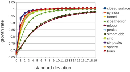
Fig. 7: Plot of noise level versus cell count for eleven implicit functions described in Appendix III. For implicit functions, noiseless volumes have average complexity close toΘ(N0.67),
and noise moves the complexity towards theΘ(N)asymptote.
visualization literature the term isosurface complexity has been used to describe the latter. Isosurface complexity is a concern in visualization applications, such as isosurface extraction (Marching Cubes [25], [26]), when processing large data sets. In this section we discuss how isosurface complexity relates to statistics of scalar fields and review recent results, then in-troduce a simple method for computing isosurface complexity based on growth rates with respect to sampling frequency.
8.1 Relation to Summary Statistics
Isosurface complexity is linked to integration and measures of surface properties. Measuring complexity adds an additional dimension to the integration, i.e. over the sampling resolution of the volume. Therefore we identify three distinct tasks that involve measuring or integrating isosurfaces.
The first task estimates algorithmic cost for rendering based on the geometric surface statistics in Section 7, i.e. cell and triangle counts, and should be treated as such. While this formed the original motivation of Carr et al. [14], in retrospect rendering cost is better predicted by the maximum number of triangles rather than the average as it represents the worst case for asymptotic analysis. We return to this in Section 8.3.
The second task computes a summary statistic for a data set, and is a volume statistic. For this, Scheidegger et al. [15] as modified in Section 6 are correct. For measuring algorithmic complexity, however, the gradient is not required.
The final task, computing fractal complexity of noisy data [23], computes complexity from fractal box span dimen-sions of a 2-manifold in a 3-space. This measures the intrinsic complexity or dimensionality of the function, and is therefore different from the previous two tasks.
8.2 Related Results
11
Year Paper Approximation(k) All Medical Measured Synthetic Implicit Functions
1994 Itoh & Koyamada [22] Triangle Count Θ(N0.67) - - - -2006 Carr et al. [14] Triangle Count Θ(N0.82) Θ(N1.05) Θ(N0.54) Θ(N0.80)
-2008 Scheidegger et al. [15] Weighted Isosurface Area Θ(N0.96) Θ(N0.70) Θ(N0.87) Θ(N0.82) Θ(N0.67)
2010 Khoury & Wenger [23] Fractal Dimensions & Cells Θ(N0.75) Θ(N0.76) Θ(N0.75) Θ(N0.73)
-2012 Duffy et al. Down-sampled Triangles Θ(N0.76) Θ(N0.77) Θ(N0.75) Θ(N0.77) Θ(N0.67)
2012 Duffy et al. Down-sampled Cells Θ(N0.71) Θ(N0.71) Θ(N0.70) Θ(N0.71) Θ(N0.65)
Scheidegger et al. [15] then argued that average isosurface complexity should account for the gradient and introduced the Co-Area formula. They used gradient weighted isosurface area to estimate k, which yielded a growth rate of Θ(N0.96). Scheidegger et al. [15] also showed that for clean implicit functions the growth rate is approximately Θ(N23), but that noise increases this. We know from Section 6 that gradient weighting gives us volume statistics: they are therefore not an appropriate measure of algorithmic complexity.
Khoury & Wenger [23] estimated a growth rate ofΘ(N0.75) by measuring the fractal dimensions of isosurfaces using cell intersections to approximate k. They count active cells because the cell counts are independent of the specific approximation methods used in isosurface reconstruction. Furthermore, they showed the fractal dimension of an isosurface is proportional to the topological noise in the data. They measured topological noise for an isosurface by computing the number of connected components and dividing by the edge intersections to correct for the dependency on isosurface area.
8.3 Asymptotic Analysis Approach
In this section we introduce a new method for measuring isosurface complexity based on a multi-scale approach. We use multiple down-sampled versions of sixty data sets to compute the growth of k as a function of N: a method suggested but not implemented by Khoury & Wenger [23]. As the lattice density increases, we measure the active cell and triangle counts at each resolution. The growth rate for each isosurface is then found from the slope of a log-log least squares line, and shown in Table 2 and Figure 7. As we see in Table 2, these approximations are similar to the prediction by Itoh & Koyamada [22]. From the variation in results, we see that the approximation chosen for isosurface reconstruction affects the computed growth rate, as predicted by Khoury & Wenger [23]. In addition to this we compute average cell count complex-ity for eleven implicit functions and add synthetic Gaussian noise in Figure 7. This verifies the result of Scheidegger et al. [15] for implicit functions. Noiseless volumes have average complexity of approximately Θ(N0.67). Adding noise to the volume moves the complexity towards the Θ(N) asymptote. The list of data sets used can be found in Appendix III.
In practice, average complexity does not have a clear mean-ing. Instead, implicit functions tend to have smooth interfaces between regions in the data, so their complexity measures are not representative of real data. For real data, peaks representing significant features tend to be distributed asymmetrically with large standard deviations. Thus, while implicit functions give a lower bound, and an upper bound of O(N)is provable, Khoury & Wenger [23] showed that the expectation is intermediate between these bounds and fractal in nature.
In Section 8.1 we noted that worst case performance should be used to predict algorithmic cost. For isosurface extraction this means taking the isosurface with the maximum growth
rate. We also note that computing the average isosurface growth rate for a given data set has very little meaning for two reasons. Firstly, average isosurface growth does not reflect how the user interacts with the isosurface extraction algorithm and may not represent a statistically significant feature in the data. Secondly, averaging implies integrating over the range of the data set and may compute the growth rate of an isosurface that does not exist when dealing with quantized data.
We therefore compute the average worst and best case growth rates from a population of 60 data sets, a subset of the 77 data sets in Appendix III. Data sets with a dimension less than 64 samples were excluded to maintain sufficient sample density when down-sampling, i.e. a data set 128×256×32 would be excluded. In practice, the average worst case for down-sampled cells is estimated at Θ(N0.87)for all real data sets, Θ(N0.89) for medical,Θ(N0.89) for measured, Θ(N0.83) for synthetic andΘ(N0.76)for implicit functions. The average best case for down-sampled cells is estimated atΘ(N0.42)for all data sets Θ(N0.44) for medical, Θ(N0.42) for measured,
Θ(N0.41)for synthetic andΘ(N0.23)for implicit functions.
9
C
OMPARISON WITHP
REVIOUSM
ETHODSIn previous sections, we established that histograms and other volume statistics provably converge to the interval volume measure, that active cell counts converge to isosurface area, and that other surface statistics empirically converge to iso-surface area. It remains to test whether adding homogeneous cells to the computation makes any significant difference.
We start with the Marschner-Lobb [27] dataset at 413
resolution. We compared the histogram with the statistics reported by Carr et al. [14], by Scheidegger et al. [15], and the updated volume statistics in Equation 22 and Equation 27. For clarity, volume statistics based on cell intersections are shown on the left of Figure 10, while those based on weighted isosurface areas are shown on the right.
In these figures we see that, as previously reported, his-tograms give poor approximations of interval volume measures at low resolutions, and that volume statistics give smoother estimates. Misleadingly, the active cell count reported by Carr et al. [14], shown in blue, appears to give the same distribution as the other statistics, presumably because the gradient in the Marschner-Lobb signal is fairly uniform. Moreover, although there are minor differences between the results of the formula reported by Scheidegger et al. [15] and Equation 22 and Equation 27, there is little to choose between them in practice. At higher resolution, in Figure 9, we see that the histogram has converged to the same result as the other volume statistics, but that the simple count of intersected cells has converged to a different result. We also see that, at the margins of the distribution, Equation 22 and Equation 27 converge slightly better than the statistics from Scheidegger et al. [15].
[image:12.612.74.536.37.105.2]0.000 0.002 0.004 0.006 0.008 0.010 0.012 0.014
Cell Intersection Statistics for Marschner Lobb 41 Data Set
Histogram Carr 06 Scheidegger 08 Duffy 12 (Eq 23)
isovalue
fr
e
u
q
e
n
y
c
0.000 0.002 0.004 0.006 0.008 0.010 0.012 0.014
Isosurface Area Statistics for Marscher Lobb 41 Data Set
Histogram Carr 06 Scheidegger 08 Duffy 12 (Eq 28)
isovalue
fr
e
u
q
e
n
y
[image:13.612.78.536.57.203.2]c
Fig. 8: Comparison of volume statistics for 41×41×41 resolution sampling of the Marschner-Lobb test signal. As in previous work, it is apparent that volume statistics of low-resolution data are of better quality than histograms.
0.000 0.002 0.004 0.006 0.008 0.010 0.012 0.014
Cell Intersection Statistics for Marschner Lobb 256 Data Set
Histogram Carr 06 Scheidegger 08 Duffy 12 (Eq 23)
isovalue
fr
e
u
q
e
n
y
c
0.000 0.002 0.004 0.006 0.008 0.010 0.012 0.014
Isosurface Area Statistics for Marscher Lobb 256 Data Set
Histogram Carr 06 Scheidegger 08 Duffy 12 (Eq 28)
isovalue
fr
e
q
u
e
n
y
[image:13.612.74.535.248.397.2]c
Fig. 9: Comparison of volume statistics for 256×256×256 resolution sampling of the Marschner-Lobb test signal. At high resolutions, the histogram has converged reasonably well, and no advantage is seen from the use of volume statistics. Minor differences are visible when homogeneous cells are added to the computations.
0.000 0.002 0.004 0.006 0.008 0.010 0.012 0.014
Cell Intersection Statistics for Monkey MRI T1 Data Set
Histogram Carr 06 Scheidegger 08 Duffy 12 (Eq 23)
isovalue
fr
e
u
q
e
n
y
c
0.000 0.002 0.004 0.006 0.008 0.010 0.012 0.014
Isosurface Area Statistics for Monkey MRI T1 Data Set
Histogram Carr 06 Scheidegger 08 Duffy 12 (Eq 28)
isovalue
fr
e
u
q
e
n
y
c
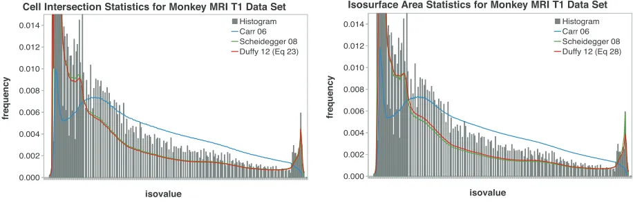
Fig. 10: Comparison of volume statistics for Monkey-MRI-T1 data. Here, the data is of very uneven quality, and the updated computation with homogeneous cells shows a marked improvement compared to previous work. Moreover, the difference between surface statistics (blue) and volume statistics becomes apparent.
an MRI scan of a monkey. Again, the simple count of inter-sected cells is clearly a different result from either histogram or volume statistic. Since we have already concluded above that this is actually a surface statistic, this poses no difficulty. But, when we compare the cell intersection statistics, we see that the computation in Scheidegger et al. [15] struggles with
the uneven quantization of the underlying data, resulting in a sequence of cusps rather than the smoother line that results from counting homogeneous cells as well.
[image:13.612.77.535.458.607.2]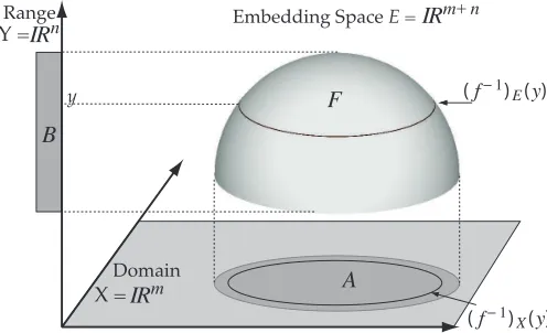
![Fig. 4: In (a) and (b), a spherical distance field was sampled and quantized to the range [0-20]](https://thumb-us.123doks.com/thumbv2/123dok_us/7976122.201074/8.612.73.543.51.298/fig-b-spherical-distance-eld-sampled-quantized-range.webp)