FGP in Multi objective Non Linear Fractional Optimization Model including Triangular Fuzzy Numbers



Abstract: The motivation behind this paper is to propose method to obtain compromized solution of Non-Linear fractional Optimization Model. In this paper, Multi-level multi-objective fully quadratic fractional optimization model (ML-MOFQFOM) is studied in which various objective functions are involved, generally have conflicting nature. FGP approach is being used to solve ML-MOFQFOM involving triangular fuzzy numbers. This paper deals with the ML-MOFQFOM in which fuzzy model

converted into deterministic form through the help of



-cuts where



is the combined choice of all objective functions. An algorithm and examples are also presented to validate the proposed method.

Keywords :



-Level set., FGP, Fully Quadratic Fractional Programming, Multi-level Multi-objective programming,

I. INTRODUCTION

ML-MOFQFOM is a hierarchical decision structure which arises in many areas like corporative planning, healthcare centre, production planning and in many other areas also. In ML-MOFQFOM, a decision maker unit is present at each level and it is almost impossible to fully satisfy each decision maker due to their conflicting nature. So, in that case priorities of DMs and compromised level of DMs make us to reach at a solution using FGP Approach. DMs having high priorities appears at First Level (FLDMU) and then according to their priorities they become the part of Second Level Decision Maker Unit (SLDMU), Third Level Decision Maker Unit (TLDMU) and so on. This paper deals with the model in which each objective functions and constraints are from fuzzy environment. So firstly they transferred into the traditional (Crisp) form by using



-cut. In ML-MOFQFOM, FLDMU has power over one decision variable, SLDMU has power over other decision variable and like that nth level decision maker unit has power over decision variable which is different from all (n-1)th levels decision variables.

The intention of this research is to reveal the method to solve ML-MOFQFOM in such a way that solution obtained is acceptable to each DMs at each level. FGP approach in this model brings a path to reach at the

Revised Manuscript Received on September 03, 2019

Dr.DeepakGupta, Maharishi Markandeshwar (Deemed to be University), Mullana-Ambala,India,

Email: [email protected]

Dr.SuchetKumar, Govt. Sec. Smart School, Fatta Maloka (Mansa), Education Department (Punjab), India,

Email: [email protected]

Namrata Rani, Maharishi Markandeshwar (Deemed to be University), Mullana-Ambala,India,

Email: [email protected]

satisfaction level of DMs. Fractional programming model is the fractional optimization model in which ratio of two function is optimized such as in profit/cost, doctor/patient, student/cost,inventory sales and so on.

Over the past few years, a number of methods had been given by many researchers in solving BLMP [3,17]. Sakawa[15] introduced interactive fuzzy programming for two level linear fractional programming problems. Parametric multi-level multi-objective fractional programming problem solution is given by Osman et al.[9]. Pramanik and Roy[14] uses fuzzy goals for solving MLPP. Linear fractional programming problems via Goal Programming adopted by Pal BB [13] and Kornbluth [4]. MLMO linear fractional problem studied by Lachhwani [6]. Kumar[5] introduced the concept of penalty function for solving Multi-objective decision making problem. Baky IA[1][2] offered a method to solve Bi-level and Multi-level Multi-objective programming problem a via FGP algorihtm. Over the past few decades, the study of multi-level programming problems with fuzziness involved in their objectives has become the major area of interest for researchers. It is useful to all those models where it is not easy to determine the crisp values due to vagueness and uncertainty involved in the information. Mishra[8] studied bi-level linear fractional programming problems using weight method. Osman[10,11,12] introduced various method to solve MLPOFPP. Shih[16] FGP approach in solving multi-level programming problem(MLPP). Multi-objective programming in fuzzy enviornment had been introduced by Lee[7] in which Pareto optimality concept.

Throughout this paper, an attempt is made to solve ML-MOFQFOM with Fuzzy demands which occurs due to uncertainty involved in the coefficient of DMs as well as of constraints. The choice of



-cut helps in this case to fix the values of coefficients. Further membership function which appear as the fuzzy goal are converted into simpler form which again become the part constraints to obtain most preferrable compromised solution. In the end, an examples are also provided to show the utilization of the proposed approach.

I. PRELIMINARIES

In this section, some useful definitions are presented.

1)



-cut of Fuzzy set:

Let ( ,X _A%( ))x be a Fuzzy set. Then defuzzified set

corresponding to



is

FGP in Multi-objective Non-Linear Fractional

Optimization Model including Triangular Fuzzy

Numbers

 

A

%

_

=



x



X

/



_A%

(

X

)



 



;



[0,1]

 

A

%

_

includes all those points for which membership function greater than or equal to



.

Some properties of



-cuts are: 1.

For

 

 

=

( ),

( ) a

=

( ),

( )

A

L

A U

A

nd

B

L B U

B

 



 



















%

%

%

%

%

%



A

%



B

%



_

= ( )

A

%





( )

B

%





A

%



B

%



_

= ( )

A

%

_



( )

B

%

_

  

A

c

( )

A

_



c









%

%

 

=

( ) ,

( ) =

( ),

( ) i

0

( ),

( ) i

< 0

A

L A

U

A

L A

U

A

f

L A

U

A

f

  



 

 















































%

%

%

%

%

%

%

Where



is a scalar.

2.



- cut for Triangular Fuzzy number

A

=





, ,

b m



%

with membership function

is

( ) =

0

A

x

x

b

b

b

x

m

m

x

x

m b

otherwise















_

 



_{ }





 







%

 









=

/

( )

=

(1

),

(1

) ; [0,1]

A

A

x

x

b

b m











 

 











%

%

II. PROBLEM FORMULATION

MLPM deals with the model in which decision maker unit are present in hierarchy at each level having dominance over decision variables. Decision maker unit is a vector of objective functions with fuzzy parameters subject to the constraints which are quadratic having intersection as convex flexible region.

Consider a hierarchical system consists of l DMU in which

ith level DM control over the variable



1 2



=

,

,...,

ni ni

;1

i i i i

x

x x

x



 

i

l

.Where



1 2



₁

=

,

,...,

_l n

w

n=

l _i

;

_i

1

x

x x

x



here



n n

 

i

and

F x x

%

_i

( ,

_{1 2}

..., )

x

_l



F

%

_i

:

     

n1 n2

...

nl ti ;

= 1, 2,...,

i

l

is the vector of

i

th level fractional quadratic decision maker. Mathematical model of maximization type of ML-MOFQFOM is represented as.



1 2 1



1 1 1 1

1 1

1

st

: max

= max

( ),

( ),...,

t

( )

x x

level

F

f

x f

x

f

x









1442 443

%

1442 443

%

%

%

... (1)

Has control over decision variable

x

₁



1 2 2



2 2 2 2

2 2

2

nd

: max F = max

( ),

( ),...

t

( )

x x

level

f

x f

x

f

x









1442 443

%

1442 443

%

%

%

... (2)

Has control over decision variable

x

2

...



1 2



: max F = max

( ),

( ),...,

t

( )

th _l

l l l l

x_l x_l

l level

f

x f

x

f

x









1442 443

%

1442 443

%

%

%

... (3)

Has control over decision variable

x

l Subject to the constraints

:

T

=

; 1

k k k k k

C

x F x T x

G

b

k

m



 

 





_{ }

 

 

_

 

%

%

%

%

_{... (4)}

( )

( ) =

( )

=

P

B

M

j

j i

i j

i

j T j j j

i i i i

g

x

where f

x

h x

g

x

x



x



%

%

_%

%

%

%

%

h =

_ij T

Q

_ij

C

_ij

M ; 1

_ij

, 1

_i

and

%

x

%

x



%

x



%

 

i

l

 

j

t

k

P =

j ij

, Q =

j ij

,F = f

k

i





p

yz





_{n n}

%

i





q

yz





_{n n}

 

 

%

yz _{n n}

%

_%

_%

%

k ₁

1 1

B = b

%

ij

 

 

%

ijy _n

,C = C

%

ij





%

ijy





_n

, T = T

%

 

 

%

yk _n

Here

%

p

ijyz

, q , f , b , C , t , M , N , G , b

%

ijyz

% %

yzk ijy

%

ijy

%

yk

%

ij

%

ij

%

k

%

k are fuzzy parameters. This fuzzy model is converted into crisp

(traditional) model by



-levels.

C

_k denotes the set of

constraints for

1

 

k

m

, which have convex feasible region in common. It is convential to assume that

h ( ) > 0

_ij

x



i, j a

nd



x

%

_.

III. FORMATION OF CRISP MODEL AND SOLUTION CONCEPT

In the presented ML-MOFQFOM, fuzzyness is involved in the objective functions and constraints. To move towards the target, firstly we need to convert all these into crisp one which is done by the help of



-level. Here the coefficients

k

G ,M a

% %

_ij

nd

N

%

_ij are the fuzzy numbers and

P , Q , F

%

_ij

%

_ij

%

_k

are the fuzzy matrices whose all entries are fuzzy numbers

and same happens in the vectors

B , C , b

%

_ij

%

_ij

%

_k and

T ; 1 i

%

_k

 

l

; 1

 

j

t ; 1

_i

 

k

m

,

_j

,

_j

,

_j

,

_j

,

_j

,

_j

,

G_{k M N P Q F B}

i i i i i i



%



_%



_%



_%



_%



_%



_{% C}j

,

b_k

i



_%



% and

T_k



% are the membership functions corresponding to

,

j

,

j

,

j

,

j

,

,

j

,

j

,

k i i i i k i i

G M

%

%

N

% %

P Q F B C

%

% %

%

b T

% %

_k

,

_k respectively.



-cut converts a fuzzy set completely in traditional set theory as defined in the preliminaries section. Let

     

 

k

S (G ), S (M ), S

_{ k  i}j _

N , S

_ij _

P , S Q ,S

_ij _{ i}j _

F ,

 

 

k

S



B , S

ij 

b

and

S

 

N

j i

 denotes the greatest

lower bound and

     

(G ),

_k

(M ),

_ij

N ,

_ij

P ,

_ij

Q ,

_ij

V

_

V

_

V

_

V

_

V

_

 

F ,

k

 

B ,

 

b

k j

i

V

_

V

_

V

_ and

V T

_

( )

_k denotes the least

upper bound of



-cut.

In minimization type problems, the upper and lower terms of objective function is replaced by lower bound and upper bound respectively as:

 

 

 

( ) =

p

B

j T j j j

i i i i

g x

%

x S

_

x



S

_

x



S

_

M

... (5)

 

 

 

( ) =

Q

C

j T j j j

i i i i

h x

%

x V

_

x V



_

x V



_

N

...(6)

In maximization type problems, the upper and lower terms of objective function is replaced by supremum and infimum respectively as

 

 

 

( ) =

p

B

j T j j j

i i i i

g x

%

x V

_

x V



_

x V M



_

... (7)

 

 

 

( ) =

Q

C

j T j j j

i i i i

h x

%

x S

_

x



S

_

x



S

_

N

...(8)

The constraints are also transformed into the crisp sets as follows :

1

:

T

T

G

b ;1

m

k k k k k

C

x F x

%



%

x



%



%

 

k

... (9)

changes into

 

 

 

 

:

T

F

T

G

V b

k k k k k

C

x S

_

x



S

_

x



S

_



_

...(10)

1

1

 

k

m

Similarly

:

T

T

G

b

k k k k k

C

x F x

%



%

x



%



%

...(11)

1 1 2

K = m



1, m



2,..., m

Changes into

C :

_k

x

T

V (F )

_{ k}

x



V (T )

_{ k}

x



V (G )

_{ k}



S ( )

_

b

_k

...(12)

1 2

K =

m



1,...

m

The constraints with equal sign appear twice in the proposed model as follows:

2

:

T

T

G =b ; K = m

1,..., m

k k k k k

C

x F x

%



%

x



%

%



..(13)

Changes into

:

T

V (F )

( )

(

)

k k k k

C

x

_

x V T x V G



_



_



S

_

... (14)

2

=

1,...,

k

m



m

and

 

:

T

S (F )

( )

(

)

k k k k k

C

x

_

x



S T x

_



S G

_



V b

_

...(15)

2

=

1,...,

k

m



m

Thus the objective function and constraint defined earlier together forms the deterministic model known as



-(MOFQFOM) formulated as :







 



_

_

1

1 1

1 2 1

1 1 1

1 2 ₁

1 1 ₁

[1

] : max F ( )

= max

V (

( )) V (

( ))

V (

( ))

,

,...,

S

( )

S

( )

S

( )

st

x x

t

t

level

x

g x

g

x

g

x

h x

h x

h

x



  

  

















1442 443 1442 443

... (16)

Has control over decision variable

x

l







 



_

_

2

2 2

1 2 ₂

2 2 2

1 2 ₂

2 2 2

[2

] : max F ( )

= max

V (

( )) V (

( ))

V (

( ))

,

,...,

S

( )

S

( )

_S

_{( )}

nd

x x

t

t

level

x

g x

g

x

g

x

h x

h x

_h

_x



  

  

















1442 443 1442 443

...(17)

Has control over decision variable

x

2 Continuing like this,







 



_

_

1 2

1 2

[

] : max F ( )

= max

V (

( )) V (

( ))

V (

( ))

,

,...,

S

( )

S

( )

_S

_{( )}

th

l

x_l x_l

t_l

l l l

t_l

l l l

l level

x

g x

g

x

g

x

h x

h x

_h

_x



  

  





















1442 443 1442 443

...(18)

Has control over decision variable

x

l

subject to

 

:

T

V (F )

( )

(

)

k k k k k

C

x

_

x V T x V G



_



_



S

_

b

...(19)

1 1

=

1,

2,...,

k

m



m



m

 

:

T

S (F )

( )

(

)

k k k k k

C

x

_

x



S T x

_



S G

_



V b

_

... (20)

1 2 2

= 1, 2,...,

,

1,

2...,

k

m m



m



m

0

x



_.

IV. CHARACTERIZATION OF MEMBERSHIP FUNCTIONS In this paper, to obtain solution for



-(ML-MOFQFOM), fuzzy goal are formed by membership functions for each DM

at the aspired



-level. Membership functions



 

f

ij _

;



1 i

 

l

;1

 

j

t

_i



corresponding to every DM are defined with the help of aspiration level and lower tolerance limit which are the

individual maximum and minimum in case of maximization type problem and individual minimum and maximum in minimization type problems, as





H = max f ( )

_ij _ij

,

x A

x

_

i j







1442 443

... (21)





= min f ( )

;

,

j j

i i

x A

L

x

_

i j







1442 443

...(22)

=1

=

m

k k

where A

_

_I

C

For maximization type problems,

H

_ij and

L

_ij gives the aspiration level (upper tolerance limit) and lowest acceptable level (lower tolerance limit) of achievement respectively. It is

logical to assume that any value of



f

ij

( )

x



_



H

ij

;



i j

,

are highly acceptable and any value of



j

( )



j

i i

f

x

_



L

are

absolutely unacceptable. So the membership function is defined as :



 















1

( )

( )

( ) =

( )

( )

0

j j

i i

j j

i i

j j j j

j i j j i i i

f_i

i i

j j

i i

f

x

H

f

x

L

f

x

L

f

x

H

H

L

f

x

L

 

 





_



_



_

_



_









... (23)

= 1, 2,... ; = 1, 2,...,

_i

i

l j

t

For minimization type problems,

L

_ij and

H

_ij gives the aspiration level and acceptable level of achievement

respectively. Further any value of



f

ij

( )

x



_



L

ij are

acceptable and any value of



j

( )



j

i i

f

x

_



H

will be

absolutely unacceptable Then the membership function is formulated as:







 





_



_





( )

=

0

( )

( )

( )

( )

( )

1

j j i f_i

j j

i i

j j

i i _{j j j}

i i i

j j i i

j j

i i

f

x

f

x

H

H

x

f

x

L

f

x

H

H

L

f

x

L





 

 





_







_

_













... (24)

In the same way, membership functions for the decision vectors of top level are defined as

 

_{   }

 

 

     

 

1

=

0

k k

i i _H

k k

i i

k L k k k

k i _{k k} i _L i i _H

x_i

i _H i _L

k k

i i _L

x

x

x

x

x

x

x

x

x

x

x

x





_



_



_

_













...(25)

(1

1)

(1

_i

)

i

l

k

n

  

 

Or

     

_{   }

     

 

 

0

=

1

k k

i i _H

k k

i i

k H k k k

k i _{k k} i _L i i _H

x_i

i _H i _L

k k

i i _L

x

x

x

x

x

x

x

x

x

x

x

x





_







_

_













... (26)

(1

1)

(1

_i

)

i

l

k

n

  

 

For maximization and minimization type problems respectively.

Where

 

_ik

H

x

represents the value of

x

_ik which yield highest value and

 

_ik

L

x

represents the value of

x

_ik which yield lowest value of the objective functions.

V. FUZZY GOAL PROGRAMMING APPROACH In



– (ML-MOFQFOM), every DM is interested to satisfy its own objective function which is obtained finding individual maximum and minimum. In FGP approach, aspiration level appears as the fuzzy goal. FGP approach tries to satisfy every DM objective upto the accepting level. These fuzzy goals having the aspired level unity is expressed as



j

( )



= 1

,

j i ij ij

f_i

f

x



U

V

i j



_



_



_

...(27)





1

( )

= 1

,

j

k i ik ik

f

f

x



u

v

i k



_



_



_

...(28)

Where

U

_ij

,

V

_ij

,

u

_ik

,

v

_ik



0

and

= 0,

= 0

, ,

ij ij ik ik

U





V



u





v





i j k

Here membership function for

x

_ik are linear but for



j

( )



i

f

x

_ these fuzzy goals are non-linear and become complex to solve. To avoid these calculations, we will make it simpler as follows:



j

( )



= 1

,

j i ij ij

f_i

f

x



U

V

i j



_



_



_

... (29)



( )



= 1

j j

i i

ij ij j j

i i

f

x

L

U

V

H

L





_



_





...(30)







( )



= 1

j j j

i i i ij ij

W

f

x

L

U

V



 







...(31)

Where _j

1

_j

=

_ij

i i

W

H



L

...(32)









( )

= 1

( )

j i

j j

i j i ij ij

i

g x

W

L

U

V

h x





 























...(33)

 

( )



 

  

( )

 

( )

=

 

( )

j j j j j j j

i i i i i ij i ij i

W g x

L h x

_

h x

U

h x

V

h x

   

 









j

( )



j



 



=



j

( )



i i i ij ij i

W j g

x

_



L

x

_



U







V





h

x

_

...(35)

Where,

U

ij

=



h

ij

( )

x



_

U

ij

 



and

V

ij

=



h

ij

( )

x



_

V

ij

 



 

 

 





 

 

 





 

 

 





=

j T j j j

i i i i

j T j j j

i i i i ij

T j J j

ij i i i

W

x V P

x V

B

x V

M

L

x S

Q

x

S

C

x

S

N

U

V

x S

Q

x

S

C

x

S

N

  

  

  

 























...(36)

 

 

 





 

 

 





(1

)

= 0

j T j j j

i i i i

j T j j j

i i i i

ij ij

W

x V P

x V

B

x V

M

L

x S

Q

x

S

C

x

S

N

U

V

  

  

 





 













...(37)

 

 

 





 

 





 

 

=

T j j j j j

i i i i i

j j j j

i i i i ij ij

j j j j

i i i i

x W V P

L S

Q

V

B

x

W V

B

L S

C

x U

V

L S

N

W V M

  

 

 

 

























...(38)

=

T j j j

i i ij ij i

x R x



E x U









V





G

...(39)

Where

L

_i



j

= (1



L

_ij

)

 

 

=

j j j j j

i i i i i

R

W V

_

P



L S



_

Q

...(40)

 

 

=

j j j j j

i i i i i

E

W V

_

B



L S



_

C

...(41)

 

 

=

;

,

j j j j j

i i i i i

G

W V

_

N



L S



_

M



i j

...(42)

Thus according to Karnbluth and Stewer [4] amd pal et. al[13], fuzzy goals becomes simpler .

Here,









=

j

( )

=

j

( )

ij i ij ij i ij

U





h

x

_

U



and V





h

x

_

V



as

U

_ij

,

V

_ij



0

and



h

ij

( )

x



_

F R

 





so this

implies

U

_ij





,

V

_ij

 



0

and

U

_ij



V

_ij

= 0

gives

= 0; ( = 1, 2,..., ,

= 1, 2,..., )

ij ij i

U







V





i

l j

t

The equations obtained above appears as constraints in the determining model as:

=

;

,

T j j i

i i ij ij j

x R x



E x U









V





G



i j

...(43)

with

U V

_ij

,

_ij



0

and

U

_ij







V

_ij





= 0.

In order to find the statisfactory compromised solution, the objective is to minimize the linear combination of negative

deviational variables

 

U

_ij



 which will be minimum when ij

U

is minimum.

= 0,

ij

U

 implies the full achievement of

membership goal while

U

_ij

= 1

implies the zero achievement of membership goal and

U

_ij



[0,1]





=

1

( )

ij

ij _j

i

U

U

h

x













...(44)



h

_ij

( )

x



_



U

_ij





;

i

= 1, 2,..., ,

l

t

= 1, 2,...,

t

_i

...(45)

This type of condition for positive deviational variables







V

_ij

i

= 1, 2,..., , = 1, 2,...,

l j

t

_i



is not necessary as

there non-negative value stands for full achievemnt of fuzzy goal.

Now the final model for





(

MLMOFQFOM

)

via FGP approach obtained as :

[Final Model ]





1

= = =1 =1

=

t

l i _{l n}

j i

i ij ik ik ik

i t j i i k

MinZ



W U

 



 



w

v





u



...(46)

   

1

=

; 1

< , 1

ik _{k k} i

i _H i _L

w

i

l

k

n

x



x



 

...(47)

subject to

:

T

(

)

( )

(

)

( )

k k k k k

C

x S F x S T x

_



_



S G

_



V b

_

...(48)

1 1

=

1,

2,...,

k

m



m



m

=

T j j j

i i ij ij i

x R x



E x U









V





G

...(49)

= 1, 2,

, ,

= 1, 2

,

_i

i

K

l j

K

t

   

k k

= 1

ik i _H i _L ik ik

w



_

x



x



_



u





v



...(50)

= 1, 2,...,1, = 1, 2,...

_i

i

j

n



h

ij

( )

x



_

U

ij







...(51)

= 1, 2,..., ; = 1, 2,...,

_i

i

l j

n

0

x



= 0,

0,

0

,

ij ij ij ij

U







V





U







V





 

i j

0,

0,

= 0

,

ik ik ik ik

u





v





u





v





i k

_.

Thus final model provides the compromised solution of



-(MLMOFQFOM) at decided value of



. If majority of DM doesn't agree with the compromised solution then value of



need to be modified and again final model is obtained.

VI. ALGORITHM TO EXPLAIN PROCEDURE FOR

OBTAINING SOLUTION OF



-(MLMOFQFOM)

Following the given algorithm, the compromisedsolution of





(

MLMOFQFOM

)

can be found.

Step 1. Decide the value of



in agreement of all DMS.. Step 2. Use (5-15) to Convert the given

(

MLMOFQFOM

)





into the crisp model.

Step 3. Calculate the individual maximum and minimum of

all DMs



f

_ij

( )

x



_



i j

,

Step 4. Define upper and lower tolerance limits

H

_ij and

L

_ij

for each decision makers at all levels.

Step 6. Define membership function _j



_ij

( )



f_i

f

x





for i

level and _k

 

_ik x_i

x



for i.

Step 7. Find all the weights

W

_ij as defined in (32). Step 8. Apply all the process (27-42 ) to make each membership goal simpler.

Step 9. Find the weights W_ik for decision variables x_ik. Step 10. Increase value of i and Repeat the process through step 5 until last level comes then go to step 10.

Step 11. Solve FGP final model (46-51) as defined above.

Step 12. If all the DMs agree with the solution obtained then consider it otherwise go to step14 otherwise to to step 13.

Step 13. Modify the value of upper and lower tolerance

limits

H

_ij and

L

_ij at all levels and go to step 5.

Step 14. Stop with the satisfactory solution obtained for all decision makers at all levels.

VII. NUMERICALEXAMPLE

Here we deal with some examples to make clear the proposed FGP approach.

Example 1 :

[ 1st level ]

2 2 2

1 2 3 1

2

1 2

2 2 2

1 1 2 3 1

2

1 2

1

1

4

5

10

,

1

3

5

max

1

1

4

5

10

1

3

5

x

x

x

x

x

x

x

x

x

x

x

x

x

















_

_









_

_

_

_

_









_

_







1442 443

%

%

%

%

%

%

%

%

%

%

%

%

%

%

%

%

2

,

3

where x x solves

[ 2nd level ]

2 2

1 2 3

2

2 1

2 2 2

2 1 2 3 3

2

2 1

1

2

5

7

,

1

3

1

max

3

1

1

7

8

1

3

1

x

x

x

x

x

x

x

x

x

x

x

x















_

_









_

_

_

_

_









_

_







1442 443

%

%

%

%

%

%

%

%

%

%

%

%

%

%

%

3

where x solves

[ 3rd level ]

2 2 2

1 2 3

2

3 2

2 2 2

3 1 2 3 2

2

3 2

1

2

1

9

,

1

5

2

max

1

4

1

6

7

1

5

2

x

x

x

x

x

x

x

x

x

x

x

x















_

_









_

_

_

_

_









_

_







1442 443

%

%

%

%

%

%

%

%

%

%

%

%

%

%

%

subject to

2

1 2 1 3

4

x



7

x x



2

x



35

%

%

%

%

_,

2 3 3

3

x x



14

x



20

%

%

%

,

2 1 2

7

x



8

%

x x



8

%

%

,

1 2 3

1

x



1

x



3

x



6

%

%

%

%

1

0,

2

0,

3

0

x



x



x



Where, the fuzzy parameters are given by :

1 = (0,1, 2,), 2 = (1.5, 2, 2.5), 3 = (2,3, 4),

%

%

%

4 = (3.5, 4, 4.5),5 = (4,9,5,5.1), 6=(6,6,6),

%

%

%

7=(6,7,8), 8=(7.5,8,8.5),9 = (8.7,9,9.1),

%

%

%

10=(9.9,10,10.1), 19=(13,14,15),

%

%

20=(19.8,20,20.1),35 = (34,35,36)

%

%

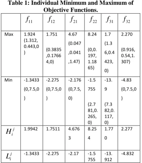
Solution : By processing according to the steps in the algorithm, the solution is obtained as :

Firstly, let us assume that all DMs agreed at



-level of 0.8. So, converting the fuzzy model into deterministic we obtain

2 2 2

1 2 3 1

2

1 2

2 2 2

1 1 2 3 2

2

1 2

0.8

0.8

3.9

5.02

10.0

,

0.8

2.8

4.98

max

0.8

1.9

0.8

5.02

10.1

0.8

2.8

4.98

x

x

x

x

x

x

x

x

x

x

x

x

x

















_

_









_

_

_

_

_









_

_







1442 443

2

,

3

where x x solves

[ 2nd level ]

2 2 2

1 2 3 3

2

2 1

2 2 2

2 1 2 3 3

2

1 1

0.8

1.9

1.9

5.02

7.2

,

1

3

1

max

2.8

0.8

0.8

7.2

8.1

0.8

2.8

0.8

x

x

x

x

x

x

x

x

x

x

x

x

x

















_

_









_

_

_

_

_









_

_







1442 443

%

%

%

3

where x solves

[ 3 rd level ]

2 2 2

1 2 3

2

3 2

2 2 2

1 1 2 3 2

2

3 2

0.8

1.9

0.8

9.02

,

0.8

4.98

1.9

max

0.8

3.5

0.8

6

7.2

0.8

4.98

1.9

x

x

x

x

x

x

x

x

x

x

x

x















_

_









_

_

_

_

_









_

_







1442 443

subject to

2

1 2 1 3

3.9

x



6.8

x x



1.9

x



35.2

2 3 3

2.8

x x



13.8

x



20.02

1 2 3

0.8

x



0.8

x



2.8

x



6

x

1



0,

x

2



0,

x

3



0