Application of photogrammetry for spatial free surface elevation and velocity measurement in wave flumes

Original Article

Corresponding author:

Alan Fleming, Australian Maritime College | NCMEH, University of Tasmania,

3

Swanson Building, B11, Launceston Tasmania, 7250, Australia

4

Email: [email protected] 5

Application of photogrammetry for

spatial free surface elevation and velocity

measurement in wave flumes

Alan Fleming

, Brian Winship

, Gregor Macfarlane

1 _{Australian Maritime College, University of Tasmania, Tasmania, Australia}

10

11

Abstract

12

This paper presents a method for obtaining the spatial free-surface elevation and velocity 13

field for the water surface in a wave flume over a relatively large measurement area for 14

this type of application (approximately 1.5 m x 1.5 m). The technique employs 15

proprietary videogrammetry software to post-process stereo images captured by multiple 16

synchronised machine vision cameras. Dimensional resolution and other limitations are 17

similar to that experienced for Particle Imaging Velocimetry (PIV) systems (𝑥, 𝑦

18

resolution of 2 mm). Imaging of the free surface was enabled by the use of millions of 19

bespoke slightly positively buoyant fluorescent flakes. Ultraviolet light (UV) was used as 20

the primary light source to excite the fluorescent flakes. Reflected UV light was 21

attenuated by a high-pass filter fitted to the cameras so that only the emitted light from 22

the fluorescent flakes was visible. 23

The software was validated using a simple linear translation experiment. An application 24

is demonstrated for the radiated wave field generated from a submerged sinusoidal 25

heaving sphere for two cases: one single and five consecutive oscillations. Results agree 26

with linear wave theory which indicates that the floating flakes had minimal impact on 27

the water surface particle motion at the scale tested. 28

It is therefore concluded that spatial measurement of the free-surface elevation and 29

velocity using the method presented has good resolution over a large measurement field. 30

The flakes were found to follow the free-surface well, but the measurement area is 31

constrained to where the pattern of flakes exists in the image. Hence, application of 32

floating markers is not suitable for experiments with significant outflow/upwelling which 33

Keywords

1

Digital Image Correlation, Videogrammetry, wave flume, surface flow, experimental, 2

velocity field, spatial free surface measurement. 3

Introduction

4

Accurate measurement of water surface elevation in wave flumes and towing 5

tanks is fundamental to experiments performed in those facilities. Commonly employed 6

single point surface elevation measurement techniques include contact measurement 7

(float/water surface following, resistive/capacitive style wave probes) and non-contact 8

methods (ultrasonic and optical)1 or indirect methods such as the laser slope gauge2. The 9

single point measurement systems are generally regarded as accurate (sub-mm accuracy) 10

when properly calibrated. 11

The single point measurement techniques can be extended for spatial 12

measurement of surface elevation by using arrays of the single point devices. For 13

example Stratigaki3 had an array consisting of 41 resistance type wave probes to measure 14

intra-array effects between scale model wave energy converters while Fleming et al.4 15

employed an array of five wave probes to measure the free-surface in an oscillating water 16

column. More recently O’boyle et al.5 _{implemented a linear array of 32 traversing wave}

17

probes utilising repeat experiments to measure a 2D wave field water elevation in pseudo 18

irregular seas. The spatial resolution of these types of systems is constrained by electrical 19

and physical interference between individual probes which typically means a minimum 20

spacing in the range of tens of millimetres is possible. Direct measurement of surface 21

particle velocity fields by these sensors is not possible and the cost of an array of sensors 22

is directly proportional to the number of sensors in the array, so it soon becomes 23

inhibitive for arrays of tens of sensors, plus the infrastructure and time required to 24

position and calibrate them. It should also be noted that there have been significant 25

advancements in development of non-contact 2D Light Imaging and Range Detection 26

systems6,7 _{for water surface elevation measurement, but to date they still offer lower}

27

accuracy and reliability than conventional contact based methods. 28

In recent years various image based systems have been developed and 29

implemented at various scales for the spatial and temporal measurement of water surface 30

elevation2,8–14, particle velocity15–17, or both simultaneously18–20. One way to categorise 31

these imaging based methods for spatial surface measurement is by considering the 32

different properties of light at the interface of two different fluids8 (air and water). The 33

main phenomena exploited include; direct observation (emission), specular reflection (off 34

the water surface), and refraction of light through the air/water interface. Generally each 35

method exploits only one of those optical properties, where the presence of other objects 36

appearing as image processing artefacts diminish the quality of the calculated result. For 37

example; most methods that directly image the free-surface require quality images of a 38

textured free-surface or distinct particles. Any presence of light as specular reflection or 39

refraction (for example; visible objects below the free-surface) will diminish the solved 40

Direct imaging based techniques can be considered the most advanced and robust 1

of these methods, which in part is due to the wider adoption of the methodology. Typical 2

methods include digital image correlation (photogrammetry)9,21–23, Particle Imaging 3

Velocimetry (PIV)15,18,19, and Particle Tracer Velocimetry (PTV)16,20,24. Commercially, 4

there are several turn-key systems available for capturing and processing data of this 5

type. However implementation of any of these systems for use in hydrodynamic facilities 6

will have similar technical challenges in directly imaging the free-surface. Arguably the 7

main technical challenge is to minimise the presence of specular reflection and unwanted 8

visible objects below the free-surface. The free-surface in hydrodynamic facilities such as 9

towing tanks and wave flumes may also contain insufficient features for satisfactory 10

image correlation without additional treatment8. 11

Turney et al.19 overcame reflection and refraction imaging problems to measure 12

interfacial particle velocities of 40 micron fluorescent seeding particles in a wind wave 13

flume by rendering the water opaque with dye and use of a ‘blue light’, thereby imaging 14

only the near-surface fluorescent seeding particles. The method requires the entire 15

experimental volume to be dyed and seeded, so is only feasible in modestly sized 16

facilities such as the 2.5 m3 of that study. 17

In the field of full-scale wave measurements some groups have recently 18

improved stereo videogrammetry algorithms to identify and compensate for specular 19

reflection, including the release of an open source software referred to as Wave 20

Acquisition Stereo System (WASS)9. The WASS software has been shown to be 21

effective for full scale measurement of water waves in a large measurement area (30 m x 22

30 m)22. The algorithm to deal with specular reflection relies on the Lambertian 23

assumption, so is most reliable with diffused light2, which also requires the cameras to be 24

mounted with a parallel viewing axis. Zavadsky et al.2 applied WASS in a small wind 25

wave flume for a measurement area of 0.25 m x 0.40 m and reported that measurements 26

had more noise than a wave gauge, but found that wave statistical results were similar. 27

They also emphasised the difficulty in producing appropriate illumination in a closed 28

laboratory. 29

Methods have been developed based on specular reflection of an image projected 30

on the water surface13,25. Kiefhaber et al.25 used specular reflection to their advantage in a 31

novel stereo imaging approach where two cameras were mounted within infrared LED 32

arrays and focused on the same region. Their system uses an inverted light path with two 33

cameras and two UV LED arrays, where each camera is mounted in an LED array. Each 34

camera and matching LED array have the same light axis and are angled toward the 35

measurement area so the alternate camera and UV LED array are in the nominal path of 36

the reflected light. Each camera is sampled in turn while the alternate LED array is 37

illuminated. In this way an inverted light path is formed. The method was shown to be 38

reliable for a measurement area of 30 x 20 cm, but scaling to large measurement areas 39

would be subject to illumination/light source complications and the occurrence of 40

dropout (absence of reflections) would increase. 41

Systems that utilise refraction of light at the free-surface indirectly measure the 42

elevation from wave theory. Generally, the methods place the camera above the water 1

surface and image a target on the tank bottom. Moisey et al10 _{describe a Schlieren method}

2

which utilise a single camera system directly over a submerged array target. The method 3

is inexpensive to implement and well suited for non-intrusive measurement of small 4

waves but is unable to resolve strong curvature and only applies to weak deformations10, 5

furthermore the method requires a clear optical path to the tank floor. The same method 6

was later applied by Damiano et al.11 to investigate a bouncing droplet, which 7

demonstrates the usefulness of the system for non-intrusive and inexpensive small scale 8

experiments. Aureli et al.14 _{utilise co-located colour and infrared CCD sensors with a}

di-9

chromatic mirror to provide co-registered images to measure slope of the air-water 10

interface. The author’s state that the method may easily be extended to larger facilities 11

since the method does not require a telecentric system; however, a backlit checkerboard 12

target must be placed at or below the tank bottom. Engelen et al.12 utilise a similar 13

experimental setup, but employ a stereo camera in place of the co-registered cameras. 14

Gomit et al.26 measured spatial elevations of ship wake with a stereo PIV like setup with 15

two cameras mounted above the free-surface as a stereo pair and a third camera below the 16

free-surface to provide a reference image, the water was seeded with typical PIV tracer 17

particles. Extension of PIV based systems to large measurement areas is generally 18

considered not feasible since the laser power is normally a limiting factor for field of 19

view size in PIV based experiments. 20

Image based measurement of the free surface in larger experimental facilities, 21

where the measurement area is defined in the order of metres rather than centimetres, is a 22

non-trivial task. In such facilities the water is typically clean (transparent) and the surface 23

is a specular reflector. A photograph taken of these facilities will usually show only the 24

floor of the tank and reflection from one or more light sources but very little water 25

surface will be visible. Even if it was possible to exclusively image the surface, there is 26

likely insufficient texture in the image to enable reliable image correlation. The method 27

we apply to overcome these challenges in this paper combines the ideas of fluorescent 28

seeding and floating particles16,17,27_{, but we utilise weakly buoyant fluorescent wax}

29

flakes27 with a typical direct image correlation of stereo image pairs. Considering the 30

scale of these experiments, surface particle interaction was assumed to have minimal 31

impact on the experimental outcome. 32

In the methodology section we briefly describe the software, followed by a 33

detailed description of the experimental setup, a simple verification test and 34

quantification of bias error. In the results section we present a case study of processed 35

surface flow data relating to the radiated wave field generated by a heaving sphere. 36

Conclusions on the limitations and benefits of the system follow. 37

38

Methodology

39

For free-surface measurement we utilise a typical stereo imaging setup and 40

process data with the software DaVis 8.2,and the add-on packages StrainMaster DIC / 41

GMBH. The software uses Digital Image Correlation (DIC) to identify corresponding 1

points in stereoscopic camera image pairs to map the objectives’ surface. Through a 2

calibration process, the position of the two cameras relative to the experimental area is 3

determined as well as some characteristics of the lens distortion. Then with an iterative 4

Least Square Matching (LSM) algorithm equivalent pixels in the two cameras are 5

identified, from which it is possible to deduce the 3D surface, and the relative pixel 6

locations. Sub-pixel interpolation is achieved with cubic B-spline interpolation. The LSM 7

algorithm is then applied to a subsequent 3D image to deduce the velocity of the particles 8

with an affine transform. The processing uses a region grow pyramid from a user defined 9

seeding point. 10

Experimental setup

The experiments reported here were conducted as part of an extensive 12

experimental campaign within an Australian Renewable Energy Agency funded project 13

(grant A00575). The primary objective of the project was to develop and validate a web 14

based planning tool for use by Governments and wave energy device developers to 15

understand the impact on performance of changing the spacing between wave energy 16

devices. Part of the project was a campaign consisting of over 1000 experimental runs 17

which utilised the photogrammetry method described in this paper to image the water 18

surface around different array configurations of wave energy converter analogues. A full 19

description of the experimental setup is not necessary here, however the interested reader 20

can obtain further detail on the project in the following references 28–30. The broader aim 21

of the research reported here was to obtain quality water surface elevation and velocity 22

measurements utilising publically available DIC software. It is worth noting that the open 23

source WASS software described by Bergamasco et al.9 was only publically available 24

after the project was finalised, but also doesn’t offer surface velocity measurements. 25

Experiments were performed in the Australian Maritime College’s Model Test 26

Basin (MTB) which is 35 m long, 12 m wide and capable of 1 m depth but here was filled 27

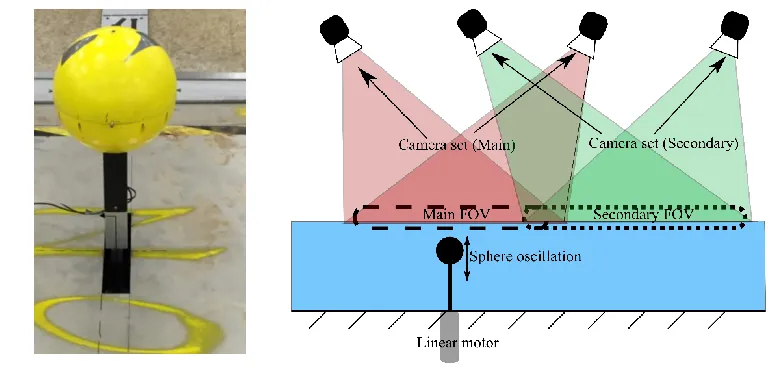
to a depth of 0.6 m. A linear motor driven sphere of 250 mm diameter was positioned at 28

the approximate centre of the MTB. At mid-stroke, the top of the heaving sphere was 515 29

mm above the basin floor. Infrastructure to support the linear motor in position was 30

placed in a bespoke pit so that only the sphere and supporting post were located above the 31

basin floor (FIG. 1 left). The purpose of the sphere was to oscillate in sinusoidal motion 32

to radiate waves in a coherent fashion in either the heaving or surging configuration. 33

Results presented here are limited to the heaving configuration. 34

The videogrammetry system consisted of two sets of machine vision cameras with 35

overlapping fields of view to provide a larger measurement area (FIG. 1 right). Wide 36

angle lenses were used to increase the field-of-view, as the camera positioning was 37

restricted by the ceiling of the test facility. The cameras were positioned on a single cross 38

beam which was supported at each end by vertically mounted stepper motor driven linear 39

slides. This enabled easy translation of the cameras during the calibration process while 40

maintaining relative position between the cameras. The first camera system was 41

positioned to monitor the area directly over the sphere and consisted of two Basler Beat 42

with a Birger adapter (to adjust lens aperture) and an orange longpass filter (Midopt 550 1

nm Filter M82.0x0.75). Cameras were connected to a PC fitted with two Silicon Imaging 2

microEnable IV frame grabbers and synchronisation boards. Images were later down 3

sampled to a resolution of 2048 x 1536 (3 megapixel) to enable faster post processing 4

time while maintaining the desired resolution. The second camera pair were centred on an 5

area offset by -1300 mm in the 𝑥 direction and consisted of two Basler ACE (acA2040-6

90um) 12 bit, 4 megapixel USB3 cameras, each fitted with a Kowa 6 mm LM6HC, 1.5 X 7

Edmund optics lens extender and c mount orange longpass fiter (Midopt LP550-25.4). 8

Cameras were connected to a PC via 10 m long fibre optic USB3 extension cables. 9

Image acquisition was synchronised via a hardware clock at a rate of 25 frames 10

per second. Commencement of data acquisition coincided with initiation of linear motion 11

via a separate hardware trigger. Images for both sets of computers were copied to RAM 12

and stored using in house software. 13

14

15

FIG. 1: Left - 250 mm diameter sphere on post in-situ in the MTB without water. Linear

16

motor and support frame are hidden below the floor plate. Right: Representation of

17

camera layout and sphere location.

18

Surface markers

As mentioned in the introduction, imaging of the free-surface in wave flumes and 20

towing tanks is a non-trivial task. For this purpose, in the order of one million flakes were 21

manufactured in house consisting of a blend of paraffin wax, carnauba wax and 22

ultraviolet fluorescent pigment in the ratio of 90:7.5:2.5 by weight respectively. The 23

approximate dimensions of the flakes (FIG. 2 bottom left) were 5 mm x 5 mm and 1 mm 24

thick, and had specific gravity of approximately 0.93, each flake occupied between 4 and 25

10 pixels of an image to produce a textured image typical as portrayed in FIG. 2 – centre. 26

The irregularity of the flakes was sufficient to provide the texture necessary for the 27

photogrammetry software. A high coverage factor was found to give best processing 28

wetted, after approximately three days of immersion in water, almost the entire flake was 1

submerged with only the occasional corner of flakes breaching the surface, or where 2

particles physically overlapped. 3

A floating fence was used to contain and concentrate the wax flakes within a 4

roughly rectangular area of approx. 7 m x 6 m meaning approximately 40 kg of flakes 5

were required. The fence was fabricated from 100 mm wide strips of 3 mm thick closed 6

cell foam with evenly spaced clumped lead weights used to provide a suitable righting 7

moment to keep the fence vertically aligned (FIG. 2 left top and right). Position of the 8

fence was maintained by generating a restoring force through 12 separate vertical nylon 9

lines equally spaced around the fence. Each nylon line passed over a pulley connected to 10

one of two overhead trusses positioned over the front and rear of the area of interest. A 11

clump weight was suspended in air from each nylon line to generate the restoring force 12

such that the attachment point of the nylon line on the fence was directly below the 13

pulley. Ballasting of the fence was adjusted to minimise interference of the fence on the 14

generated wave fields and was found to be relatively transparent. 15

Although results are not provided on experiments utilising the in-built wave 16

generator in the MTB in this paper, it is worth mentioning that the fences were observed 17

to be highly transparent to long-crested waves, the fence would move and deform under 18

the wave action with the nearby water particle motion with minimal radiation or 19

absorption of the incoming wave. For short-crested waves the fence drifted down-wave 20

with the water particle displacement related to the action of Stokes’ drift, thus limiting 21

experimental time to approximately 40 seconds as the clumped weights reached the 22

extent of their travel (which caused significant interference to the incoming wave field). 23

Excitation of the fluorescent wax flakes was achieved with a total of 12 ultraviolet 24

stage wash lights (each consisting of an array of 54 X 3 Watt UV LEDs). The stage lights 25

were mounted on two overhead trusses and directed toward the ceiling over the area of 26

interest which was found to diffuse the light effectively to provide a sufficiently uniform 27

light signal throughout the field of view for both sets of cameras. Diffused and consistent 28

light intensity was found to improve image processing and also enables use of a lower 29

image sensor bit depth without saturation. 30

FIG. 2: Left top: A small section of the (blue) floating fence laid out flat with three lead

1

weights on the lower edge. Left bottom: Close up of flakes floating on the free surface

2

(rule scale in cm) Centre: A section of a deformed (corrected) image of the free surface.

3

Right: UV excited fluorescent flakes held in station over the measurement area contained

4

by the floating fence.

5

Calibration

The calibration process employs a calibration plate and software wizard to derive 7

the necessary camera parameters and position the cameras in space31_{. Once a calibration}

8

was performed the cameras were not moved relative to one another. A custom made 9

calibration plate (FIG. 3) of 2.4 m × 2.4 m was made from an array of equally spaced 10

dots (10 mm diameter, 50 mm spacing) from 3 layer white black white sign material to 11

fill the area of interest. The calibration plate (consisting of rigidly joined two halves of 12

1.2 m x 2.4 m) placed on a floating 50 mm thick expanded polystyrene backing. The 13

surface of the calibration plate was measured to have floating elevation of 49 mm above 14

the still water level. 15

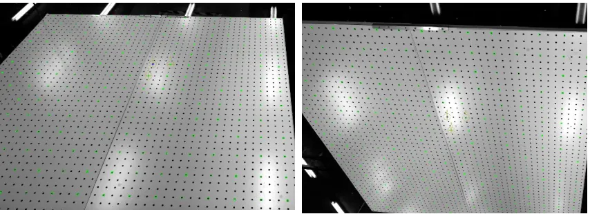
FIG. 3: View of calibration plate with selected calibration points and datum reference for

16

camera 1 (left) and camera 2 (right) (main camera set).

17

For the calibration to be valid it was necessary to acquire several “views” of the 18

calibration plate at different planes throughout the area of interest. To perform this action 19

the cameras were fitted on a cross-bar between two vertically oriented stepper motor 20

driven linear stages. The cross-beam was then raised and lowered to provide a total of 21

eight coplanar image pairs over a total vertical range of 170 mm. The sum of the 22

corrected images post-calibration (all views) from both camera sets is shown in FIG. 4. 23

Note that only every third calibration point was used for the first camera set and every 24

second calibration point was used for the second camera set (green and white circles in 25

FIG. 3) which was found to provide lower overall calibration residuals (RMS of fit). 26

1

FIG. 4: Sum of corrected images from both cameras and all views. The grey border

2

signifies the extents of the camera overlap in the measurement volume. Left: Main

3

camera set, the red grid lines are 150 mm apart. Right: Secondary camera set, the red grid

4

lines are 100 mm apart.

5

In a more typical surface flow system; (consisting of cameras fitted with lenses 6

having less distortion) the process described above would be sufficiently accurate for the 7

software to reliably run to completion. However due to the requirement for a larger field 8

of view and the constraint on the object distance, the current lenses were selected. So in 9

the case for the data acquired; attempting to process the data resulted in a failed solution. 10

The cause of the failed solution was found to be that the calibration was inadequately 11

solved by the calibration wizard. To improve the calibration beyond that produced by the 12

standard calibration wizard, a software tool “self-calibration”, available in a separate 13

DaVis 8.2 product Stereoscopic PIV, was used to improve the calibration. Not only did 14

the RMS of fit reduce from 0.66 pixels to 0.12 pixels for the main cameras but 15

importantly, the software ran more reliably. A summary of calibration details are 16

provided in Appendix A. 17

A measure of the accuracy of the calibration and DIC software can be evaluated 18

by inspecting the photogrammetry solution for the still free-surface, this is covered in the 19

following sections. 20

Image processing

Image pairs were processed using the following settings as they were found to 22

give reliable results for the datasets throughout: subset size = 21, step size = 10, 23

calculation mode = fast and maximum expected pixel displacement = 50 pixels. 24

The DIC software was validated by means of a vertical translation test during 1

which 200 images were obtained whilst the cameras were traversed in the 𝑧 direction 2

from 0 to 100 mm. Accuracy of the linear stage and its vertical alignment were not 3

quantified with sufficient accuracy to state whether the source of error presented here was 4

due to error in the photogrammetry system or misalignment of the linear translation 5

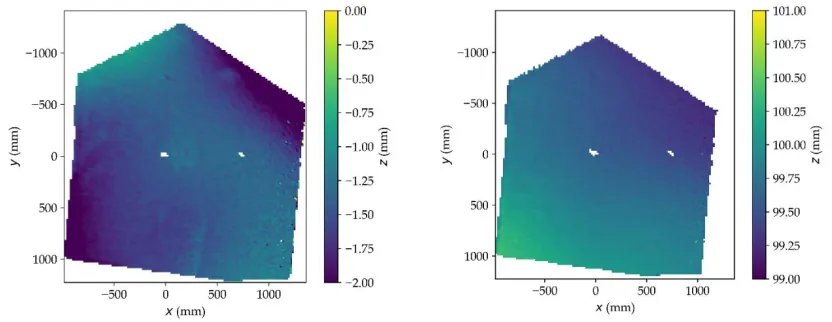
system. FIG. 5 right shows the surface solution after the camera system was lowered a 6

vertical displacement of 100 mm and the left image subtracted, the mean value is 99.7 7

mm. Crudely this equates to an estimated uncertainty in the videogrammetry system of 8

0.3 mm. The remainder surface (FIG. 5 right) is clearly not level, however examination 9

of the gradient (not shown) suggests the measured (still water) surface is flat so the error 10

can mostly be attributed to incorrect vertical alignment of the camera traverse system 11

rather than error in the stereo system or its calibration. 12

13

14

FIG. 5: Photogrammetry result from the still water surface after final calibration. Left:

15

zero image. Right: 100 mm translation in 𝒛 direction image with zero image subtracted.

16

Bias error

FIG. 5 left is an image of the still free surface after final calibration. It is clear 18

that not only is the surface not flat, the surface does not coincide with the zero plane. This 19

is partially attributed to calibration plates not being perfectly flat. In other types of data 20

acquisition systems it is typical to subtract a zero value, bias error, from the reading to 21

give the expected value 32. A zero image was developed for each camera set using a 22

collection of images of the still free-surface as follows: 23

1 Each image decimated by a reduction factor of 2;

24

2 Each image resized by 3rd order spline interpolation by a reduction factor of 6;

25

3 A median filter of size 20 is applied to each image;

26

4 Images averaged;

27

5 Missing data pixels expanded by a binary dilation of 10 pixels;

28

6 Missing data filled in using biharmonic inpaint (scikit-image inpaint);

7 Image resized by 3rd order spline interpolation by a growth factor of 12 to original

1

image size.

2

3

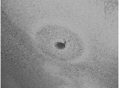
FIG. 6: Raw image from a main camera during an experiment for heaving sphere

4

showing particles are absent directly over the sphere location. Also a wave crest

5

generated by the heaving sphere is visible

6

Additionally, for the main camera set (considering the results for a heaving sphere 7

near the free surface), a circular region with a radius of 100 mm centred over the origin 8

was not able to be processed due to particles washing away from the region as a feature 9

of local currents caused by the sphere oscillation (FIG. 6). FIG. 7 shows both the zero 10

image (left) and an example of a corrected first frame (right) for the main and secondary 11

camera systems (top and bottom respectively). The remaining texture visible (FIG. 7 - 12

right) is a combination of physical texture present measured on the water surface due to 13

the presence of the fluorescent flakes, where some flakes may be sitting on top of others, 14

and residual uncertainty. Edge effects are introduced as a result of the filtering which is 15

most pronounced as can be seen by the yellow border in FIG. 7 lower right. The 16

remainder of the analysis presented will utilise data inside of the areas of the zero image 17

FIG. 7: Left: Calculated zero image to correct 𝒁 bias error. Right: Surface elevation of

1

the still water surface with the zero image (left) subtracted. Top row correspond to the

2

Main camera set and bottom row correspond to the secondary camera set.

3

Surface velocity measurements

In addition to surface elevation measurements it was possible to determine 3 5

dimensional surface displacement between frames, provided that image sequences are 6

taken with a sufficiently short time between frames. Ultimately this provides the user 7

with a velocity field of the surface, similar to Particle Imaging Velocimetry (PIV), but 8

returns the velocity for the surface rather than for a plane as is typical for PIV. 9

Preliminary results of surface flows have already been reported by the authors in 29, 10

which was used to demonstrate the surface currents expected in the vicinity of wave 11

energy converters. Because the velocity is extracted from two sequential images, the 12

velocity is the average between the subsequent frames with an uncertainty in the timing 13

of the motion equal to the interframe time (40 ms in this case) centred on the midpoint 14

between the two images. Since the velocity fields are a differential result, it is not 15

necessary (or appropriate) to subtract a zero image to correct for bias error. 16

Results

17

Results are presented in this section for two experiments of a sphere oscillating 1

vertically in sinusoidal motion for both one, and five complete cycles starting from the 2

bottom of the stroke. The sphere oscillated with an amplitude of 70 mm and a frequency 3

of 1 Hz. Sphere displacement is shown in FIG. 8. A ninth order 4 Hz low pass filter was 4

applied to the positional data to remove linear motor drive induced noise, 𝑧 = 0 mm is 5

taken as the still water level. 6

7

FIG. 8: Instantaneously position of the sphere top surface below the static water free

8

surface (z = 0 mm) where the blue solid line is a single oscillation and the dashed orange

9

line is five oscillations.

10

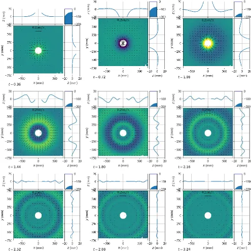
The surface radiation field for a single oscillation of the sphere is shown in FIG. 9 11

(using a reduced square window of the main camera set). The primary purpose of this set 12

of images is to demonstrate the symmetry of the radiation field, but it is also interesting 13

to note that a wave packet is generated by a single oscillation of the sphere which is 14

thought to be caused by the proximity of the sphere to the free surface. Videos of the 15

same are available as video 1 for a single oscillation and video 2 for five oscillations. 16

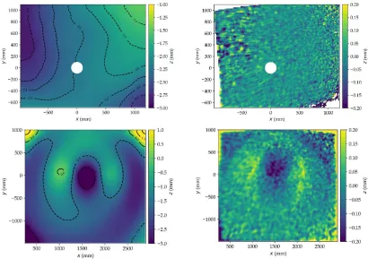
FIG. 10 : Left: is a plot of the upper and lower bounds of the free surface 17

elevation radially extending out from the origin. Waviness in the appearance of the data 18

is a feature of the rather low sampling frequency, while the discrepancy between 19

neighbouring data points is a combination of measurement error and physical 20

inconsistency in the radiated wave field. But clearly there is good agreement in data from 21

different angles, which confirms the accuracy of the bias error correction through the use 22

of a zero image. 23

FIG. 10 : Right: is a plot of the instantaneous surface amplitude from the Main 24

and Secondary camera sets at the time instances of 1 second and 3.8 seconds sliced 25

through 𝑦 = 0. There is good agreement between the two sets of data, however it is 26

apparent that the Secondary camera set is smoother than the Main camera set which most 27

notably reduces the amplitude of the measured crests and troughs of the steeper waves. 28

The cause of the reduced accuracy of the Secondary camera set may be associated with 29

the larger field of view, increased camera lens distortion (lower focal length lens) or 30

slightly smaller pixel scale factor of 0.491 pixel/mm compared to 0.544 pixel/mm of the 31

1

FIG. 9: Instantaneous water surface elevation and velocity generated by sphere heaving

2

for a single cycle at 1 Hz and 70 mm amplitude at time steps 𝒕 = 𝟎. 𝟑𝟔 , 𝟎. 𝟕𝟐, 𝟏. 𝟎𝟖, 3

𝟏. 𝟒𝟒, 𝟏. 𝟖𝟎, 𝟐. 𝟏𝟔 , 𝟐. 𝟓𝟐, 𝟐. 𝟖𝟖, 𝟑. 𝟐𝟒 from left to right and top to bottom

4

respectively. The centre white circle covers the fluid surface region where flakes were

5

missing due to the presence of surface currents. Instantaneous position of the sphere to

6

the free-surface is illustrated in the top right corner of each figure.

1

FIG. 10: Left: Radial maximum and minimum amplitudes at 45 degree intervals of

2

radiated wave field for a single sphere oscillation at 1 Hz and 70 mm. Right:

3

Instantaneous surface profile at two different time instants for the Main and Secondary

4

camera sets sliced through 𝑦 = 0 for a single sphere oscillation at 1 Hz and 70 mm.

5

The five cycle data set is used for an extended window to investigate validity of 6

overlaying data from different camera sets. Image sets from both camera sets were 7

combined on a frame by frame basis by first resizing the images to the full sized window 8

using third order spline interpolation (2 mm spacing between pixels). Images from the 9

main and secondary sets were then averaged using a weighted average technique, which 10

generated a weighting image using Gaussian blur applied to a unity array (ones) of equal 11

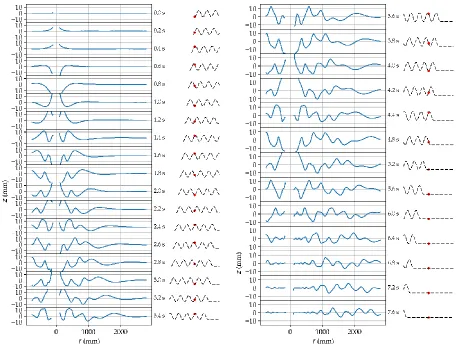
shape to the base image. FIG. 11 is a sequence of time-series snapshots of surface profile 12

taken through the centreline at 𝑦 = 0. The overlap between the two sets of data occurs at 13

1

FIG. 11: Cross-section of surface profile time-series of wave field generated by sphere

2

heaving at 1 Hz and 70 mm amplitude (5 complete cycles) composed of the merged

3

surface profile from the main and secondary camera sets. The dashed line indicates the

4

path history of the sphere and the red dot indicates the location of the sphere at that time

5

instant.

6

Given that there is periodic motion in this data set; it is possible to apply periodic 7

analysis to the time-series data such as phase-averaging or spectral analysis. In this case a 8

spectral analysis was chosen for two reasons. First, the harmonic components and phase 9

are both obtained. Second, only two cycles of data were available containing the 10

developed flow over the majority of the region of interest. This would provide an 11

inadequate amount of samples for phase-averaging to be effective. Spectral analysis using 12

Fourier Transforms is less sensitive to the number of cycles, rather, the total number of 13

samples only affects the Nyquist frequency. 14

Spectral analysis was performed on a pixel by pixel basis (similar to a method 15

described in Longo and Stern33) for the same data set used to generate FIG. 11 (𝑦 = 0)

16

but limited to the time 3 ≤ 𝑡 ≤ 5 seconds giving 51 data points per pixel. Using 3rd _order

17

spline interpolation, data was resampled to 2𝑛 = 256 data points (𝑛 = 8) to prevent zero 18

then calculated corresponding to the original timestamps using 𝜂𝑛 =

1

𝐴𝑛cos(2 𝜋 𝑛 𝜙1(𝑡 − 𝑡0) + 𝜙𝑛), where 𝜂𝑛 is the instantaneous profile at time 𝑡 relative to

2

starting time 𝑡0, and 𝜙𝑛 is the phase of the 𝑛th harmonic.

3

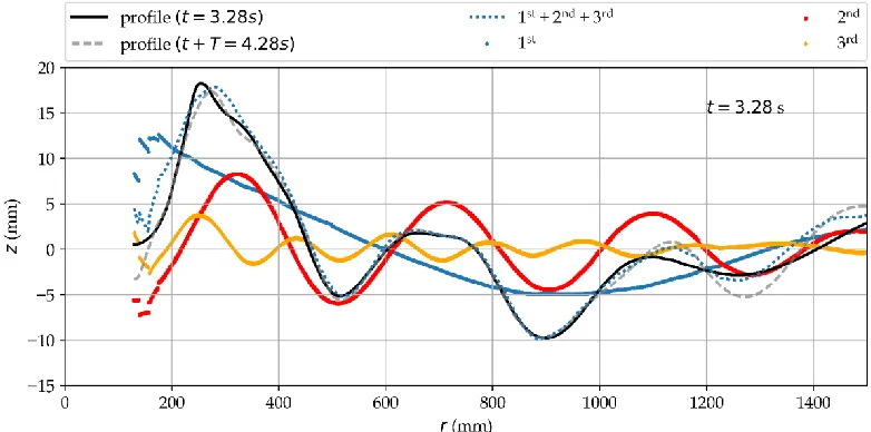
FIG. 12 is a plot of the instantaneous profile corresponding to 𝑡 = 3.28 s. Both 4

the original data and summed harmonic components are plotted so we can evaluate the 5

effectiveness to reconstruct the original wave profile. The original profile at 𝑡 = 3.28 s is 6

plotted as a solid black line and the original data from 𝑡 = 4.28 s is plotted as a dashed 7

grey line. The data points of the measured data correspond well for radius values 8

between 𝑟 = 200 mm and 𝑟 = 1000 mm, after which there is some divergence that is 9

attributed to the third order component not having propagated past the 1000 mm radius. 10

The sum of the first three harmonics are plotted as a dotted blue line. In this case the 11

harmonic analysis is shown to be effective for the region 400 < 𝑟 < 1000 mm. The 12

reason for the deviation of the fit from the data for radius 𝑟 < 400 mm is due to the 13

proximity of the sphere to the free-surface. Whereas the cause of deviation for radius 𝑟 >

14

1000 mm was due to differing wave profiles in the source data (absence of the third 15

harmonic as mentioned above). The time and distance for the propagation of the third 16

order harmonic wave component (propagating at 𝐶_𝑔 =𝑔⁄_4𝜋𝑓) can be predicted with 17

linear wave theory which equates to 780 mm (for 𝑡 = 3 s), and if the diameter of the 18

sphere is taken into consideration this appears to agree with that observed. In short, the 19

origin of the wave front should not necessarily be assumed to be 𝑟 = 0. An animation of 20

the same data is provide in video3. 21

22

FIG. 12: Profiles of the actual surface (black solid and then grey dashed for 𝒕 + 𝑻) and

23

reconstructed water surface (blue dots) of wave field generated by the sphere heaving at 1

24

Hz and 70 mm amplitude at equvalent time 𝒕 = 𝟑. 𝟐𝟖 s. First, second and third order

25

reconstructed surface are added as blue circles, orange squares, and orange diamonds

26

respectively.

27

Furthermore, it was possible to analyse the individual frequency components of 28

wavelength was directly measured and averaged from the frames available. Secondly, 1

wave celerity was calculated from the measured displacement of wave crests between 2

respective frames divided by the time between frames. Results are summarised and 3

compared to those predicted through linear theory in Table 1, agreement is within two 4

standard deviations of the measured values. 5

Table 1 : Wavelength and celerity of harmonic components of wave field generated by

6

sphere heaving at 1 Hz and 70 mm amplitude measured from Fourier analysis and

7

compared against deepwater linear wave theory.

8

Wavelength (m) Celerity (m/s)

Harmonic Experimental Linear theory Experimental Linear theory 1 1.477 ± 0.015 1.561 1.488 ± 0.143 1.56 2 0.389 ± 0.005 0.390 0.781 ± 0.059 0.78 3 0.187 ± 0.023 0.173 0.474 ± 0.062 0.52

9 10 11

Velocity field generated by heaving sphere

12

As mentioned previously, the instantaneous velocity fields are calculated from 13

adjacent image pairs, thus the time instant of the motion is averaged between the two 14

images. This also means that the most likely time instant of the displacement (with the 15

assumption of constant velocity between two images) occurs at the time instant between 16

the two images. To approximately account for time offset the velocity fields shown in 17

FIG. 9 are interpolated with 3rd _{order splines from adjacent velocity fields to closer}

18

represent the time instant at which the surface elevation was measured. 19

Utilising velocity field data instead of surface elevation FIG. 13 is similar to FIG.

20

10 but is a scatter of the maximum surface particle velocity in that data set rather than 21

elevation. The figure clearly demonstrates that wave field velocity is axisymmetric and 22

also that the maximum particle velocities diminish with increasing radius. Close to the 23

source of the wave there are a scatter of lower magnitude data points reflecting the issue 24

previously highlighted regarding floating markers washing away due to the upwelling 25

1

FIG. 13: Radial maximum surface particle velocity at 45 degree intervals of radiated

2

wave field for a single sphere oscillation heaving at 1 Hz and 70 mm.

3

Conclusions

4

Spatial measurement of the water surface in hydrodynamic test facilities will 5

continue to be an area of interest to researchers. In this paper it was demonstrated that it 6

is feasible to utilise DIC software in conjunction with floating fluorescent surface 7

markers to provide good surface elevation and velocity measurements over a 8

considerable area of 1.5 m x 1.5 m. The field of view may be extended through the use of 9

additional stereo camera pairs with no particular complication. 10

Acquisition of high resolution surface measurements enables feature extraction 11

otherwise unobtainable through point measurements, such as instantaneous snapshots of 12

free-surface elevation, true measurement of wavelength, wave group celerity and the 13

surface particle velocity field. Imaging based systems will continue to require good 14

quality artefact free images, advancements might be possible with hardware 15

improvements including noise reduction and corresponding sensitivity. 16

The main limitation found in application of this method was imaging of the free 17

surface. Utilisation of floating surface markers was found to be effective for cases where 18

station keeping of the floating markers was possible and no inflow sources (without 19

markers) exist, typical for irrotational flow such as low steepness non-breaking waves. 20

Usefulness of the method can be immediately extended through proper acquisition of 21

stereo image pairs of a textured water surface. 22

Acknowledgements

23

We thank the following for their assistance in experimental setup and data 24

acquisition throughout the project: Guy McCauley, Jeremy Ledoux, Romain Briand, Kirk 25

Meyer and Liam Honeychurch. We also thank staff at LaVision for their technical 26

support in initial processing of the data and comments on how to improve processing 27

Funding

1

This work was supported by the Australian Renewable Energy Agency Emerging 2

Renewables Program [ERP A00575 - Towards an Australian capability in arrays of ocean 3

wave-power machines]. Brian Winship was jointly funded by CSIRO Oceans and 4

Atmosphere Climate Research Centre and the Australian Renewable Energy Agency 5

(ARENA) Emerging Renewables Program (ERP A00521 – The Australian Wave Energy 6

Atlas Project). 7

References

8

1. Payne GS, Taylor J, Ingram D. Best practice guidelines for tank testing of wave 9

energy converters. The Journal of Ocean Technology 2009; 4: 38–70. 10

2. Zavadsky A, Benetazzo A, Shemer L. On the two-dimensional structure of short 11

gravity waves in a wind wave tank. Physics of Fluids 2017; 29: 016601. 12

3. Stratigaki V. Experimental study and numerical modelling of intra-array interactions 13

and extra-array effects of wave energy converter arrays. Dissertation, Ghent 14

University, http://hdl.handle.net/1854/LU-5664337 (2014, accessed 9 February 15

2017). 16

4. Fleming A, Penesis I, Goldsworthy L, et al. Phase averaged flow analysis in an 17

oscillating water column wave energy converter. Journal of Offshore Mechanics and 18

Arctic Engineering 2012; 135: 021901-[1-9]. 19

5. O’Boyle L, Elsäßer B, Whittaker T. Experimental measurement of wave field 20

variations around wave energy converter arrays. Sustainability 2017; 9: 70. 21

6. Rak G, Hočevar M, Steinman F. Measuring water surface topography using laser 22

scanning. Flow Measurement and Instrumentation 2017; 56: 35–44. 23

7. Blenkinsopp CE, Turner IL, Allis MJ, et al. Application of LiDAR technology for 24

measurement of time-varying free-surface profiles in a laboratory wave flume. 25

Coastal Engineering 2012; 68: 1–5. 26

8. Gomit G, Chatellier L, Calluaud D, et al. Large-scale free surface measurement for 27

the analysis of ship waves in a towing tank. Exp Fluids 2015; 56: 184. 28

9. Bergamasco F, Torsello A, Sclavo M, et al. WASS: An open-source pipeline for 3D 29

stereo reconstruction of ocean waves. Computers & Geosciences 2017; 107: 28–36. 30

10. Moisy F, Rabaud M, Salsac K. A synthetic Schlieren method for the measurement of 31

the topography of a liquid interface. Exp Fluids 2009; 46: 1021. 32

11. Damiano AP, Brun P-T, Harris DM, et al. Surface topography measurements of the 33

12. Engelen L, Creëlle S, Schindfessel L, et al. Spatio-temporal image-based parametric 1

water surface reconstruction: a novel methodology based on refraction. Meas Sci 2

Technol 2018; 29: 035302. 3

13. Hamachi S, Sanada Y, Toda Y. A technique to measure wave height distributions by 4

the reflected light image. Journal of the Visualization Society of Japan 2006; 26: 17– 5

20. 6

14. Aureli F, Dazzi S, Maranzoni A, et al. A combined colour-infrared imaging technique 7

for measuring water surface over non-horizontal bottom. Exp Fluids 2014; 55: 1701. 8

15. Chatellier L, Jarny S, Gibouin F, et al. A parametric PIV/DIC method for the 9

measurement of free surface flows. Exp Fluids 2013; 54: 1488. 10

16. Tamburrino A, Gulliver JS. Free-surface visualization of streamwise vortices in a 11

channel flow. Water Resour Res 2007; 43: W11410. 12

17. Kumar S, Gupta R, Banerjee S. An experimental investigation of the characteristics 13

of free-surface turbulence in channel flow. Physics of Fluids 1998; 10: 437–456. 14

18. Dabiri D, Gharib M. Simultaneous free-surface deformation and near-surface velocity 15

measurements. Experiments in Fluids 2001; 30: 381–390. 16

19. Turney DE, Anderer A, Banerjee S. A method for three-dimensional interfacial 17

particle image velocimetry (3D-IPIV) of an air–water interface. Meas Sci Technol 18

2009; 20: 045403. 19

20. Sokoray-Varga B, Józsa J. Particle tracking velocimetry (PTV) and its application to 20

analyse free surface flows in laboratory scale models. Periodica Polytechnica Civil 21

Engineering 2008; 52: 63–71. 22

21. Wanek JM, Wu CH. Automated trinocular stereo imaging system for three-23

dimensional surface wave measurements. Ocean Engineering 2006; 33: 723–747. 24

22. Benetazzo A, Fedele F, Gallego G, et al. Offshore stereo measurements of gravity 25

waves. Coastal Engineering 2012; 64: 127–138. 26

23. Ferreira E, Chandler J, Wackrow R, et al. Automated extraction of free surface 27

topography using SfM-MVS photogrammetry. Flow Measurement and 28

Instrumentation 2017; 54: 243–249. 29

24. Schanz D, Gesemann S, Schröder A. Shake-The-Box: Lagrangian particle tracking at 30

high particle image densities. Exp Fluids 2016; 57: 70. 31

25. Kiefhaber D, Caulliez G, Zappa CJ, et al. Water wave measurement from stereo 32

26. Gomit G, Chatellier L, Calluaud D, et al. Free surface measurement by stereo-1

refraction. Exp Fluids 2013; 54: 1540. 2

27. Tauro F, Porfiri M, Grimaldi S. Fluorescent eco-particles for surface flow physics 3

analysis. AIP Advances 2013; 3: 032108. 4

28. Penesis I, Manasseh R, Nader J-R, et al. Performance of ocean wave-energy arrays in 5

Australia. In: Proceedings of the 3rd Asian Wave & Tidal Energy Conference, 24 - 6

28 October 2016. Singapore, pp. 246–253. 7

29. Fleming A, Manasseh R. Experimental observation of surface currents produced by 8

WEC radiation and diffraction. In: Lewis A (ed) Proceedings of the Twelfth European 9

Wave and Tidal Energy Conference. University College Cork, Ireland: EWTEC, 10

2017, pp. 802–1–802–7. 11

30. Nader J-R, Fleming A, Macfarlane G, et al. Novel experimental modelling of the 12

hydrodynamic interactions of arrays of wave energy converters. International Journal 13

of Marine Energy 2017; 20: 109–124. 14

31. LaVision. Flowmaster - product manual for DaVis 8.3. Anna-Vandenhoeck-Ring 19, 15

D-37081 Göttingen: LaVision, 2016. 16

32. ITTC. Guide to the expression of uncertainty in experimental hydrodynamics, ITTC 17

guide 7.5-02-01-01, revision 01. 2008. 18

33. Longo J, Stern F. Uncertainty assessment for towing tank tests with example for 19

surface combatant DTMB model 5415. Journal of ship research 2005; 49: 55–68. 20

21

Appendix A

1

Table 2: Calibration factors for surface flow calibration using a software wizard standard

2

pinhole calibration and the stereo PIV “self-calibration”

3

Camera set Main (Basler Beat) Secondary (Basler Ace)

Calibration Standard

Pinhole calibration

Final Pinhole calibration

Standard Pinhole calibration

Final Pinhole calibration Camera 1 Camera 2 Camera 1 Camera 2 Camera 1 Camera 2 Camera 1 Camera 2 RMS of fit (pixels) 0.66308 0.11614 0.12424 0.52474 0.10170 0.11274 Camera configuration Focal length (mm) 24.436 24.436 9.1471 9.20065

Pixel Size (mm) 0.011 0.011 0.0055 0.0055

Pixel aspect ratio 1 1 1 1

Calibration plate position (z=0 mm) Translation Tx (mm) -794.621 -794.621 -800.161 -754.183 -277.546 261.3 -1071.22 -546.302 Ty (mm) 259.202 259.202 265.417 -72.8042 395.249 343.449 76.6162 -75.9249 Tz (mm) 2786.72 2786.72 2768.65 2452.2 2367.79 2335.27 2696.03 2280.31 Rotation Rx (deg) -4.97765 -4.97765 -4.5612 -3.80478 -15.4652 -13.1571 -15.2976 -13.5028

Ry (deg) 45.7358 45.7358 45.6992 -40.9343 14.0031 -12.1781 14.4464 -12.1141 Rz (deg) -97.313 -97.313 -96.8922 -92.7693 -4.40905 2.7473 -3.49725 3.77372 Size of dewarped image 1273 x 1911 1275 x 1925 2777 x 2817 1844 x 1902 Camera scale origin x0 (pixel) 536.733 534.733 1348.35 504.64

y0 (pixel) 684.59 691.59 765.61 708.69

Scale factor (pixel/mm) 0.542211 0.544092 0.742396 0.491319 Image distortion Principal point xp (px) 1700.68 1700.68 1702.18 1707.18 1018.11 1011.35 1015.37 1014.59

yp (px) 782.157 782.157 779.945 812.495 1072.82 1062.08 1071.88 1058.79

Radial distortion 1st _{order 0.997144 0.997144 0.062119 0.87402 11.3782 9.86013 8.40527 8.34727}

2nd _{order 0 0 0.286693 -0.00198 -0.94744 -0.33996 0.078699 0.229095} 4