A new class of multiscale lattice cell (MLC) models for spatio-temporal evolutionary image representation

This is a repository copy of A new class of multiscale lattice cell (MLC) models for

spatio-temporal evolutionary image representation.

White Rose Research Online URL for this paper:

http://eprints.whiterose.ac.uk/74620/

Monograph:

Wei, H.L., Billings, S.A. and Zhao, Y. (2007) A new class of multiscale lattice cell (MLC)

models for spatio-temporal evolutionary image representation. Research Report. ACSE

Research Report no. 963 . Automatic Control and Systems Engineering, University of

Sheffield

[email protected] https://eprints.whiterose.ac.uk/ Reuse

Unless indicated otherwise, fulltext items are protected by copyright with all rights reserved. The copyright exception in section 29 of the Copyright, Designs and Patents Act 1988 allows the making of a single copy solely for the purpose of non-commercial research or private study within the limits of fair dealing. The publisher or other rights-holder may allow further reproduction and re-use of this version - refer to the White Rose Research Online record for this item. Where records identify the publisher as the copyright holder, users can verify any specific terms of use on the publisher’s website.

Takedown

If you consider content in White Rose Research Online to be in breach of UK law, please notify us by

A New Class of Multiscale Lattice Cell (MLC) Models for

Spatio-Temporal Evolutionary Image Representation

H. L. Wei, S. A. Billings and Y. Zhao

Research Report No. 963

Department of Automatic Control and Systems Engineering The University of Sheffield

Mappin Street, Sheffield, S1 3JD, UK

A New Class of Multiscale Lattice Cell (MLC) Models for

Spatio-Temporal Evolutionary Image Representation

H. L. Wei, S. A. Billings and Y. Zhao

Department of Automatic Control and Systems Engineering

The University of Sheffield

Mappin Street, Sheffield

S1 3JD, UK

[email protected], [email protected]

Abstract: Spatio-temporal evolutionary (STE) images are a class of complex dynamical systems that evolve over both space and time. With increased interest in the investigation of nonlinear complex

phenomena, especially spatio-temporal behaviour governed by evolutionary laws that are dependent

on both spatial and temporal dimensions, there has been an increased need to investigate model

identification methods for this class of complex systems. Compared with pure temporal processes, the

identification of spatio-temporal models from observed images is much more difficult and quite

challenging. Starting with an assumption that there is no apriori information about the true model but

only observed data are available, this study introduces a new class of multiscale lattice cell (MLC)

models to represent the rules of the associated spatio-temporal evolutionary system. An application to

a chemical reaction exhibiting a spatio-temporal evolutionary behaviour, is investigated to

demonstrate the new modelling framework.

1. Introduction

In the real world, spatio-temporal evolutionary (STE) phenomena is found in many diverse fields

of science and engineering including biology, chemistry, ecology, geography, medicine, physics, and

sociology (Kaneko 1993, Jahne 1993, Silva and Principe 1997, Astic et al. 1998, Bascompte and Sole

1998, Czaran 1998, Spors and Grinvald 2002, Dimitrova and Berezney 2002, Berezney et al. 2005,

Dolak and Schmeiser 2005). To analyse or imitate STE phenomena, several efficient representations,

for example the well known cellular automata (CA) (Wolfram 1994, Adamatzky and Bronnikov 1990,

Adamatzky 1994, 1996, 2001, Ilachinski 2001), cellular neural networks (CNNs) (Chua and Yang

1988a, 1988b, Roska and Chua 1993, Chua et al. 1995, Crounse and Chua 1995, Thiran et al. 1995,

Chua and Roska 2002), and coupled map lattice (CML) models (Kaneko 1989, 1993), have been

proposed. In these representations, it is often assumed that the associated mathematical model

structure, along with the model parameters, is known, so that the model can be used to describe or

analyse some specific phenomena. However, the evolution laws associated with real-world STE

phenomena may not always be completely known, and evolution rules need to be acquired from

observed data of images or patterns. Hence, in recent years, the identification of spatio-temporal

models from observed data has received much attention and several efficient identification methods

and algorithms have been proposed, see for example Adamatzky and Bronnikov (1990), Adamatzky

(1994, 1996, 1997), Sitz et al. (2003), Coca and Billings (2001), Mandelj et al. (2001), Billings and Coca (2002), Billings and Yang (2003), Yang and Billings (2003), Billings et al. (2006).

This study considers the spatio-temporal model identification problem, where it is assumed that

there is no apriori information about the true model structure and only imaged data are available.

Motivated by the successful applications of the wavelet-based multiscale and multiresolution analysis

approach (Mallat 1989) in classical signal and image processing (Mallat 1998, Unser 1999), as well as

in dynamical process modelling (Billings and Coca 1999, Billings and Wei 2005a, 2005b, Wei and

Billings 2004a, 2004b, 2006, Wei et al. 2004, 2006), and also inspired by the easy tractability of

conventional coupled map lattice models (Kaneko 1989, 1993), this study aims to introduce a novel

multiscale lattice cell (MLC) model for STE system identification. Unlike in a typical wavelet-based

multiscale or multiresolution dynamical modelling approach, where the elementary building blocks are

strictly chosen to be some dyadic wavelets, in the new MLC model, the choice of the prototype

functions are permitted to be very flexible, any functions including wavelets, B-splines and Gaussian

type functions can be chose as the elementary building blocks as long as there is strong evidence that

the functions possess desirable properties and can lead to a good model for a given modelling problem.

In most existing wavelet models for dynamical systems, the scale and shift parameters are restricted to

a dyadic lattice. Dyadic wavelet models are proved to be perfect for general static signal representation,

in that dyadic wavelets, along with associated scale functions, can often form orthogonal (orthonormal)

1992). An important property of an orthonormal decomposition is that the well known Pareval’s

theorem holds, that is, the energy of a signal is conserved, without any loss, in the wavelet coefficients.

For the STE dynamical system modeling problem, where observations are often sparse in the problem

space, however, a dyadic lattice may not usually be an optimal choice. In addition, data used in dyadic

wavelet models for nonlinear dynamical systems often need to be compressed or normalised to [0,1],

to simplify the associated modelling procedures (especially for the determination of the wavelet shift

parameters) (Billings et al. 2006). Although data normalization is frequently used in many modelling

approaches and can often simplify the associated modeling procedures, normalization may, at the

same time, change the physical meanings of the signals to be modeled. This may be undesirable for

some applications where variables are required to preserve their physical dimension. In the new MLC

model, data normalisation procedures become unnecessary.

The MLC model is composed of a number of basis functions; the feature of each individual

function is determined by three factors: the scale (dilation) parameter, the shift (translation) parameter,

and the coefficient weighted on the associated function. For a chosen elementary building block (the

prototype function), the task of MLC model identification involves as least three aspects: the

determination of the scale and shift parameters; the determination of the model structure and

complexity, that is, the determination of which and how many basis functions should be included in

the model; and the estimation of the weight coefficients. A new simple unsupervised histogram-based

clustering algorithm is introduced; this method can be used to determine the scale and shift parameters

of individual functions that will be used to form an initial full MLC model; this full model is in

general highly redundant. A forward orthogonal regression (FOR) learning algorithm (Billings and

Wei 2007a, Wei and Billings 2007), implemented using a mutual information estimation method, is

then applied to refine and improve the initial MLC model by removing redundant basis functions.

2. The MLC Model

In this study, the two-dimensional case, which has obvious physical meanings and is widely

applied in practice, is taken as an example to illustrate how to construct an MLC model. For simplicity,

only the zero-input (autonomous) case is considered here. In an autonomous STE system, no external

input image is imposed, and the output image at any time t is due exclusively to the initial conditions

and the evolution of the pattern. Model representations for these situations can easily be extended, in a

straightforward way, to other more complex cases.

2.1 The lattice cell model

Assume that the 2-D image or pattern produced by an STE system, at the time instant t, consists of

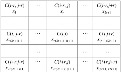
Table 1. The (2r+1)×(2r+1) neighbourhood

C(i-r, j-r)

x1

… _{C(i-r, j)}

xr

… _C(i-r,j+r)

x2r+1

… … … … …

C(i, j-r)

xr(2r+1)+1

… _C(i,j)

xr(2r+1)+(r+1)

… _C(i,j+r)

x(r+1)(2r+1)

… … …

C(i+r,j-r)

x2r(2r+1)+1

… _C(i+r,j)

x2r(2r+1)+(r+1)

… _C(i+r,j+r)

x(2r+1) (2r+1)

Following Chua and Roska (2002), let S_rt(i,j)be the sphere of influence of the radius r of cell

) , (i j

Ct , at the time instant t, defined as

} |} | |, {| max : ) , ( { ) , ( 1 ,

1 i p j q r j i C j i S J q I p t t

r = _{≤ ≤ ≤ ≤} − − ≤ (1)

where t=1,2, …, i=1,2, …, I, j=1,2, …, J, and r is a non-negative integer number indicating how many

neighborhood cells are involved in the evolution procedure. The sphereSrt(i,j) is sometimes referred

to as the (2r+1)×(2r+1) neighbourhood. Let s_i,j(t)∈Rbe the state variable representing the cell

) , ( ) ,

(i j S i j

Ct ∈ _rt . From the definition of S_rt(i,j), a total of (2r+1)2state variables are involved in (1),

see Table 1, where the symbol C(i,j) will be used to indicate cells at an arbitrary evolution time instant.

Let si_,j(t) be the (i,j)th cell to be updated at time t. A wide range of STE systems can be described

by the discrete-time, discrete-space and continuous-state spatio-temporal difference equation of the

form below )) ( , ), 2 ( ), 1 ( ( ) (

,j lag

i t f t t t n

s = s − s − L s −

, ), 1 ( , ), 1 ( , ), 1 (

( , − L , − L , − L

= f si−r j−r t sij t si+r j+r t

, ), 2 ( , ), 2 ( , ), 2 ( _{, ,}

, − − L − L + + − L

− t s t s t

s_{i rj r ij i r j r}

)) ( , ), ( , ), ( , ,

,j r lag ij lag i r j r lag r

i t n s t n s t n

s_{− −} − L − L _{+ +} − (2)

where f is some nonlinear function,n_lagis the time lag, defined as a positive integer, indicating how

many past images or patterns are involved in the evolution procedure, and s(t−k) is the state vector

formed by the (2r+1)2 state variables relative to the patterns at the time instant (t-k) with k=1,2, …,

lag

n , that is,

)] ( ), ( , ), ( [ )

(t−k = s_i−r,j−r t−k L s_i,j t−k s_i+r,j+r t−k

Note that the general lattice cell representation form (2) includes, as special cases, most typical

coupled map lattice models. For convenience of description, introduce d single-indexed variablesx_k(t)

as below

)] (

, ), 2 ( ), 1 ( [ )] ( , ), ( ), ( [ )

(t = x₁ t x₂ t x_d t = s t− s t− st−n_lag

x L L (4)

where s(t−k)=[x_{1+(k−1)(2r+1)}2(t),L ,x_k(2r+1)2(t)] for k=1,2, …, n_lag . For the case n_lag =1, the

description (4) is shown in Table 1. Also, let y(t) represent the state variable si_,j(t) corresponding to

the central cell Ct(i,j). Then, Eq. (2) becomes

)) ( ( )

(t f t

y = x = f(x₁(t),x₂(t),L ,xd(t)) (5)

In conventional coupled map lattice models, the nonlinear function f in model (2) is often assumed

to be known as some deterministic function. However, for real-word complex STE systems, a

pre-determined function f may not sufficiently characterise the underlying dynamics. It may be better to

learn, from available real observations, an appropriate model for a given STE system. The task of STE

system identification is to construct, based on available data, a model that can represent, as close as

possible, the observed evolution behaviour. Unlike constructing static models for typical data fitting,

the objective of dynamical modelling is not merely to seek a model that fits the given data well, it also

requires, at the same time, that the model should be capable of capturing the underlying system

dynamics carried by the observed data, so that the resultant model can be used in simulation, analysis,

and control studies.

2.2 The new MLC model

Inspired by the idea behind the traditional coupled map lattice models, the present study employs

an additive model structure to approximate the nonlinear function (5)

)) ( ( ˆ )

(t f t

y = x +e(t) = f1(x1(t))+ f2(x2(t))+L + fd(xd(t)) +e(t) (6)

where f_i(⋅) are some univariate nonlinear functions that need to be identified, and e(t) is some

modelling error that can be treaded as an independent identical distributed noise sequence. One

commonly used approach, for effectively reconstructing the nonlinear functions f_i(⋅), is to construct a

nonlinear approximator fˆ using some specific types of basis functions including polynomials, radial _i

basis functions, kernel functions, splines and wavelets (Leontaritis and Billings 1987, Chen and

Billings 1992, Brown and Harris 1994, Aguirre and Billings 1995, Murray-Smith and Johansen 1997,

Cherkassky and Mulier 1998, Harris et al. 2002, Wei and Billings 2004a, 2004b, Billings and Wei

2005a, 2005b). More often, models constructed using these methods can easily be converted into a

identification, because compared to nonlinear-in-the-parameters models, linear-in-the-parameters

models are simpler to analyze mathematically and quicker to compute numerically. The present study,

however, employs a family of shifted multiscale basis functions to approximate the nonlinear

maps f₁,f₂,L ,f_d in (6).

Now take a wavelet-based approximation as an example. Let ψ be a chosen mother wavelet.

Consider the family

      − = a b x a b x ψ

ψ( ; , ) (7)

where a∈R+, b∈R, and the waveletψ is admissible. The admissibility condition is depicted using

the Fourier transform ψˆ(ξ)of the function ψasC_ψ =

∫

these d functional components f_i(x_i) can now be represented as

∑∑

i x t w x t b a

f ( ( )) (_,)ψ( (); (_,), (_,)) (8)

where (,)

i j k

a and (,)

i j k

b are pre-determined scale and shift parameters, and (,)

i j k

w are the associated weight

coefficients. Equation (6) can now be written as

)) ( ( ˆ )

(t f t

y = x +e(t)

∑

=

= d

i i i x t

f

1

)) (

( +e(t)

∑∑∑

= d

i k j

i j k i j k i i j

k x t b a

w 1 ) ( , ) ( , ) (

,ψ( (); , ) +e(t) (9)

This is the initial full MLC model for the associated STE system (2). In this model the scale and shift

parameters a_k(i_,)_j and b_k(i_,)_j are restricted to a pre-specified non-dyadic lattice, which is directly

determined by using the information given by the original observation dataset. The weight

coefficientsw_k(i_,)_j, however, need to be estimated by solving the associated regression equation problem.

Some realization issues, relative to the construction of the MLC model (6), include:

• The determination of the scale and shift parameters a(_ki_,)_jand b_k(i_,)_j.

• The initial full model (9) is often redundant, so a key problem involves how to refine and improve

the model to produce a parsimonious model with good generalisation properties.

• The estimates of the weight coefficients ()

,

i j k

w are highly dependent on the given estimation dataset

3. The Determination of the Shift and Scale Parameters

3.1 The Histogram-Based Grouping Algorithm

Consider a given time series {x(t):t=1,2,L ,N₀}. Let 0

1 min min{ ()}

N t

t x

x = ₌ , 0

1 max max{ ()}

N t

t x

x = ₌

and R=[x_min,x_max]. Now the objective is to partition all the data points in the time series {x(t)}into K

groups. The grouping criterion and the associated partitioning procedure are as follows:

• Divide the interval R into k equally-spaced sub-intervals (bins); the kth bin is defined as

) ,

[ ₊₁

= k k k r r

R for k=1,2, …, K-1, and R_k =[r_k,r_k+1]for k=K, where r_k =x_min+(k−1)h and

K x x

h=( _max− _min)/ (h is referred to as the bin width).

• If x(t)∈R_k, then the t-th data point is included in the kth bin.

• Denote the number of data points contained in the kth binRkbygk.

These are the basic ideas of the commonly used histogram method. However, the determination of

the bin width and bin number K is still an open issue in histogram analysis (Wade 1997). The famous

Sturges’ rule (Sturges 1926), which has been used in default in some popular languages and software,

suggests that the total bin number be chosen to beK =1+log₂(N₀). It has been pointed out (Scott

1992) that the Sturges’ rule is more of a number-of-bins rule rather than a bin-width-oriented rule

itself, and it has been shown (Scott 1992) that the bin width produced by the Sturges’ rule leads to an

over-smoothed histogram, especially when the number of samples is large. Based on a

well-established theory (Scott 1992), two cross-validation (CV) criteria has been derived for bin width

choice. The biased CV and unbiased (least squares) CV functions are given below

∑

h (10)

∑

0 ( 1) ( )

1 ) ( ) 1 ( 2 )) ( (

UCV (11)

whereh(K)=(x_max−x_min)/Kis the bin width of K partitions. The bin width for the associated dataset

is defined to be the one that minimises the BCV or UCV vriteria. These cross validation criteria can be

used to determine the scale and shift parameters of the associated basis functions.

3.2 Choice of the Shift and Scale Parameters

For a given time series {x(t):t=1,2,L ,N0}, assume that a total of K groups have been determined

using the above histogram-based grouping algorithm, and let c_kbe the centre (midpoint) of the kth

It is known that wavelet basis functions are compactly supported or nearly compactly supported.

For example the B-splines and associated wavelets (Chui 1992, Unser et al. 1993, User 1999) are

compactly supported, while the Gaussian and the Mexican hat (or Marr) wavelets (Daubechies 1992,

Billings and Wei 2005a) are nearly compactly supported. Hence, to the wavelet transform (7), for any

scale and shift parameters a and b, there must exist a positive numberδsuch that

0 | ) , ; ( | ≈      − = a b x a b x ψ

ψ , for − ≥δ

a b x

(12)

For example, for the 1-D Mexican hat waveletψ(x)=(1−x2)exp(−x2/2) , |ψ(x)|≤0.0001 for

5 |

|x≥ δ= . Thus, for a fixed shift parameter b, the scale parameter a should not be chosen too small,

because a very scale will ‘disable’ many useful data points. On the other hand, the scale parameter a

should not be chosen too large, because a very large scale could make the associated functions become

too smooth to capture detailed dynamics of the signal.

From the above discussion, the shift and scale parameters b and a are chosen as follows:

• The number of wavelet shift parameters is chosen to be K, where K is defined using the

histogram-based grouping algorithm.

• The K shift parameters b₁,b₂,L ,b_K are chosen to be the centres of the K bins (groups).

• For each shift parameter bk, allocate a total of J scale parameters to the associated basis functions,

denote these scale parameters by a₁,a₂,L ,a_J , where a_j=2ja₀/4 for j=1,2, …, J and

K K h

a₀= ( )/ 2 .

Here, the idea of choosing a₀=h(K)/ 2K comes from Haykin (1999), where it is suggested that the

scale (bandwidth) parameter be chosen as bi bj K

K j i 2 / |} {| max 1 − = ≤ < ≤

σ . Applying the above procedure

to equation (6), yields,

∑ ∑∑

1 1 1

) ( ) ( ) ( , ( ( ); , ) )

( ψ +e(t)

∑ ∑ ∑

j ji

i k i i j k i a b t x w

1 1 1 () ) ( ) ( , ) (

ψ +e(t) (13)

where a(_ji) and b_k(i) are the scale and shift parameters, relative to the ith variablex_i(t). In model (14),

it is assumed that the time series {xi(t)}produced by the ith variablexi(t)has been partitioned intoKi

groups, and thus a total of K_i shift parameters are involved for the variablex_i(t); for each of these

initial full wavelet model (14) contains a total of M =J(K₁+L +K_d) basis functions. Model (14)

can easily be converted to a linear-in-the-parameters form below

∑

=

= M

m m

m t

t y

1

) ( )

( θ φ +e(t) =φT(t)θ+e(t) (14)

where { ( ; , (,)): 1,2, , ; 1,2, , ; 1,2, , }

) (

J j

K k

d i

a b

x i

i j k i k i

m∈ ψ = L = L = L

φ ,θ_mare model parameters, and

T M t t

t) [ (), , ( )] ( = φ1 L φ

φ and θ are the associated regressor and parameter vectors, respectively.

Notice that in most cases the initial full regression equation (14) might be highly redundant, some of

the regressors or model terms can thus be removed from the initial regression equation without any

effect on the predictive capability of the model, and this elimination of the redundant regressors

usually improves the model performance. Generally, only a relatively small number of model terms

need to be included in the regression model for most nonlinear dynamical system identification

problems. An efficient model term selection algorithm is thus highly desirable to detect and select the

most significant regressors.

4. Model Refinement Using the Forward Orthogonal Regression Algorithm

Letφm =[φm(1),L ,

T m(N)]

φ be a vector formed by the mth candidate model term in the initial full

model (15), where m=1,2, …, M. Let D={φ₁,L ,φ_M} be a dictionary composed of the M candidate

bases. From the viewpoint of practical modelling and identification, the finite dimensional set D is

often highly redundant. The model refinement problem amounts to finding, from the vector dictionary

D, a full dimensional subsetD_m ={p₁,L ,p_m} { , , }

1 im

i φ

φ L

= , where

k i

k φ

p = , i_k∈{1,2,L ,M} and

k=1,2, …, m (generally m<<M ), so that y can be satisfactorily approximated using a linear

combination of p1,p2,L ,pm as below

m m mp e

p

y=β1 1+L +β + (15)

where emis the associated model residual vector.

The orthogonal least squares (OLS) algorithm (Billings et al. 1989, Chen et al. 1989,) can be used

to determine model basis functions (model terms). In this study, however, a variation of the OLS

algorithm, called the forward orthogonal regression (FOR) algorithm, implemented using a mutual

information method (Billings and Wei 2007a, Wei and Billings 2007), is employed for model

refinement. Assume that x and y are two random discrete variables, with alphabet X andY ,

respectively, and with a joint probability mass function p(x, y) and marginal probability mass functions

) (x

p andp(y). The mutual information I(x,y) is the relative entropy between the joint distribution

  



=

∑∑

∈ ∈ ( ) ( )

) , ( log ) , ( )

, (

y p x p

y x p y

x p I

x Xy Y

y

x (16)

The mutual informationI(x,y)is the reduction in the uncertainty of y due to the knowledge of x, and

vice versa. Mutual information provides a measure of the amount of information that one variable

shares with another one. If y is chosen to be the system output (the response), and x is one regressor in

a linear model, I(x,y)can then be used to measure the coherence of x with y in the model. Several

algorithms have been proposed to estimate mutual information from observed data, see for example

Moddemeijer (1989, 1999), Darbellay and Vajda (1999), and Paninski (2003) and the references

therein.

Detailed discussions about the utility of the mutual information for model term selection can be

found in Billings and Wei (2007a) and Wei and Billings (2007). Now, let p₁,p₂,L ,p_nbe the n

selected linearly independent basis vectors after the nth step search, and letq₁,q₂,L ,q_n be a group of

orthogonal vectors, generated from the vectors p1,p2,L ,p_n , by means of some orthogonal

transformation. Following Billings et al. (1989), Chen et al. (1989), the error reduction ratio (ERR),

produced by including the nth basis vectorq_n, or equivalently by including p_n, is defined as

2 2 2

|| ||

|| || ERR

y qn n n

γ

= (17)

where 2

|| || /

, n n

n=<y q > q

γ . ERR can be used to measure the significance of individual model terms

in that it provides an index indicating the contribution made by each selected individual model term to

explain the total variance in the desired output signal.

Lete_nbe the residual vector produced at the nth search step. Similar to in the OPP algorithm, the

model residual vector e_ncan be used to form a criterion to terminate the search procedure. Following

the suggestion in Billings and Wei (2007b), the following adjustable prediction error sum of squares

(APRESS), also referred to as the adjustable generalised cross-validation (AGCV), will be used to

monitor the regressor search procedure

2

) / 1 (

) ( MSE APRESS

N n

n

n

λ −

= (18)

whereMSE(n) || n|| /N

2

e

= is the mean-square-error that is associated to the model of n model terms.

The number of regressors (wavelet functions) will be chosen as the value where APRESS arrives at a

minimum. Billings and Wei (2007b) suggest that the adjustable parameterλ be chosen between 5 and

10.

Following Billings and Wei (2007a) and Wei and Billings (2007), the mutual information based

The FOR-MI algorithm: Step 1: SetU₁={1,2,L ,M}; for j=1 to M

j

j φ

q(1) = ;

[ ] ( 0, (1))

) 1 ( j MI j

I = r q ; // Calculate the mutual information for all

// candidate basis vectors.// end for

₁ argmax{ (1)[]} 1 i I U i∈ =

l ; V₁={l₁};

1

1 φl

p = ; q₁=p₁; ₂

1 1 1 || || , q q y > < =

γ ; r₁=r₀−γ₀q₁;

2 2 1 2 1 || || || || ] 1 [ ERR y q γ = ; N N 2 1 2 || || ) / 1 ( 1 ] 1 [ APRESS r λ − = ;

Step n, n≥2: Forn=2 to M

U_n=U_n−1\V_n−1; for j∈Un

∑

I(n)[j]=MI(r_n−1,q(_jn)); //Calculate the mutual information for all // for all candidate basis vectors.// //{if ||q(_jn)||2≤ε,set I(n)[j]=0}// end for ( end loop for j )

argmax{I(n)[j]} U j n n ∈ =

l ; ={ } {arg(|| ( )||2<ε)}

∈ n j U j n n n

V l U q ;

n

n φl

p = ; qn=q(ln_n); 2

|| || , n n n q q y > < =

γ ; rn =rn−1−γnqn;

2 2 2 || || || || ] [ ERR y q_n n

n =γ ;

N N n n n 2 2 || || ) / 1 ( 1 ] [ APRESS r λ − = ;

for k=1 to n

_{, 2} || || , k k n n k r q q p > <

= , fork<n; rk,n=1, fork=n;

end for (end loop for k ) end for (end loop for n )

The FOR algorithm provides an effective tool for successively selecting significant model terms (basis

functions) in supervised learning problems. Terms are selected step by step, one term at a time. The

inclusion of redundant bases, which are linearly dependent on the previous selected bases, can be

efficiently excluded by eliminating the candidate basis vectors for which ||q(_jn)||2 are less than a

predetermined thresholdε, say 10

10−

≤

ε . Assume that a total of m significant vectors are selected,

from the triangular equation Rβ=γ , where R is an upper triangular matrix and

T m] , , , [γ1γ2L γ

=

γ with 2

|| || /

, i i

i=<yq > q

γ for i=1,2,…, m.

5. Applications

The new MLC modelling framework can be applied to identify some SPE phenomena, where the

true models are unknown and the initial full model involves a great number of ‘input’ or ‘independent’

variables. To illustrate the application of the new modelling method, the Belousov-Zhabotinsky

(Belousov 1959, Zhabotinsky 1964, Winfree 1972, Kuramoto 1984) reaction was considered here as

an example.

The BZ reaction, as an excitable medium (Adamatzky 2001, 2004), is representative of an

important class of chemical reactions exhibiting a spatio-temporal oscillatory behaviour. As a classical

example of nonequilibrium thermodynamics, the BZ reaction provides an interesting chemical model

of nonequilibrium phenomena, and the modelling and identification of these types of reactions is of

extreme interest for theoretical analysis of such phenomena.

By adopting the recipe given by Winfree (1972), an experiment resulting in a thin layer BZ

reaction was carried out in the laboratory, and a set of images were captured (sampled) with equal time

intervals during the experiment, using a digital video camera that is connected to a PC via a USB

socket. The sampled images were processed and saved as patterns with a resolution of 300 by 500

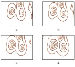
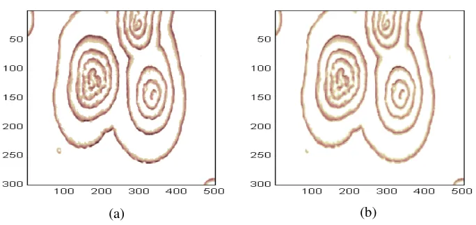
pixels. Some of these patterns are shown in Fig. 1.

The proposed MLC modelling framework was applied to these sampled images, and the objective

was to identify a mathematical model for the BZ reaction. Details of the identification procedure are

given below.

5.1 The initial model and the training data

Consider the model of the form (2), where the number of total model variables is determined by

two factors: the radius of the neighbourhood, r, and the time lag, n_lag. In the present study, the two

coefficients were chosen to be r=1, and n_lag=2. Thus, the model (2) involves a total of 18 model

variables.

The state variables_i,j(t), at the present time instant t, was initially assumed to be associated with

state variables in the past two adjacent neighbourhoods at the previous time instants t-1 and t-2. Any

two patterns, at the abutting time instants t and t-1 are called an adjacent pattern group. For an

arbitrary time instant, the data pair,{x(t),y(t)}, wherex(t)and y(t) are defined by (4) and (5), is called

a data pair. Notice that x(t)and y(t) are also implicitly associated with the spatial location indices i

and j (see Table 1). As a consequence, for any given time instant t, there would be a large number of

Fig. 1 Some snapshots for the BZ reaction at different time instants. The size of each template is 300×500(300 pixels in the vertical direction and 500 pixels in the horizontal direction). (a) t=10; (b) t=20; (c) t=30; (d) t=40.

A training dataset, consisting of a total of N=6000 data pairs, {x(k),y(k)}_k=1,2,...,_N, was generated

for model identification, where y(k) represents the value of the relevant central cell at the present time

instant, and x(k)=[x₁(k),x₂(k),L ,x₁₈(k)]T represent the values of the 18 involved cells on a squared

lattice, at the previous time instants. Data pairs {x(k),y(k)}in the training dataset were randomly

chosen from ten adjacent pattern groups that were also randomly selected from the first 40 sampled

patterns.

5.2 Determining the shift and scale parameters

Note that all the involved 18 variables come from the same system; in a statistical sense, these 18

variables, as well as the ‘output’ variable y(t), should obey the same distribution. Thus the 18 variables

could be allocated the same shift parameters. It was noticed that the values of a great number of

observations are exactly equivalent to the maximum value ymax=255. Thus, the one shift parameter was

in default chosen to be 255, and other shift parameters were determined by performing the

histogram-(c) (d)

based grouping algorithms on the associated time series {y(t)} with t=1,2, …, N, where data points

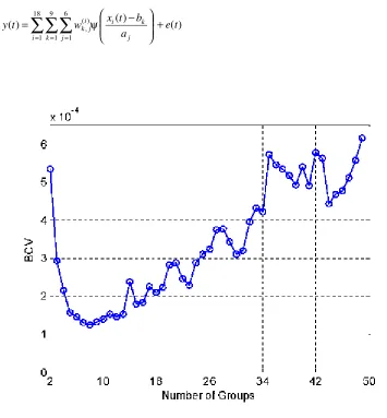
whose values are exactly equivalent to ymax, were excluded. The biased CV (BCV) criterion, shown in

Fig. 2, suggests that the optimal number of groups for the associated dataset should be chosen as 8.

Thus a total of 9 shift parameters b₁,b₂,L ,b₉ were chosen for the relevant dataset.

The Mexican hat wavelet function, defined as 2 2/2

) 1 ( )

(x = −x e−x

ψ , was used as the elementary

building block for constructing the MLC model, and the primary bandwidth for each group was

chosen to be a0=6.25. For each shift parameter bk, a total of 6 scales were to used to perform

associated wavelet transforms; denote these scale parameters by a1,a2,L ,a6, where 0

2

2 a

a_j= j− . The

initial full MLC model was thus of the form

∑∑∑

 

 

 ₋

= 18

1 9

1 6

1 ) (

,

) ( )

(

i k j j

k i i

j k

a b t x w t

y ψ +e(t) (19)

Fig. 2 The BCV criterion versus the number of groups, produced using the histogram-based clustering

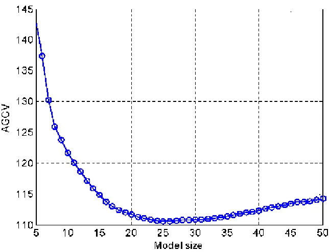
Fig. 3 The AGCV criterion versus the number of model terms (selected by using the FOR-MI algorithm).

5.3 Model refinement and performance evaluation

The initial full MLC model (19) contains a total of 972 model terms; most of the model candidate

model terms may be redundant. The initial full model thus needs to be refined. The FOR-MI algorithm

was performed, over the given training dataset, to select significant individual basis functions from the

initial model (19). The adjustable generalized cross-validation (AGCV), defined by (18) and where the

adjustable parameterλ=10, suggests that a total of 26 basis functions should be included in the final

model (see Fig. 3).

To evaluate the performance of the identified additive wavelet models, the short-term predictive

capability of the models was inspected. Denote the observation of the image (pattern) measured at the

time instant t by X(t). The k-step-ahead prediction, denoted byXˆ(t+k|X(t),X(t−1);f), where f

represents the identified nonlinear function, is the iteratively produced result by the identified model,

on the basis of X(t) and X(t-1), but without using information on observations for patterns at any other

time instants. As an example, the measurements at the time instants t=41 and 42 were used to calculate

Fig. 4 Model prediction (one step ahead) for the BZ reaction at time instant t=43. (a) Real measurement at t=43; (b) Predicted image from the model.

To quantitatively measure the performance of the identified models, the 2-D normalised

mean-square-error (NMSE), defined as below, was considered

∑∑

∑ ∑

= = = =

− − = _I

i J

j j i I

i J

j

j i j i

t s t s

t s t s t

1 1

2 ,

1 1

2 , ,

| ) ( ) ( |

| ) ( ˆ ) ( | )

(

NMSE (20)

wheresi,j(t) represent the observations at the time instant t, sˆi,j(t) represent the corresponding

predicted values from the given model, s(t)is the mean value of the patter at the time instant t, and I

and J define the size of the associated patterns. The predicted values at t=43 were compared with the

associated observations, and the normalised mean-square-error was calculated to be 0.0763.

From Fig. 4 and the NMSE value, it is clear that the identified MLC model can capture the main

spatio-temporal evolution dynamics from these real laboratory BZ reaction. The identified model can

provide very good short term predictions.

6. Conclusions

The multiscale lattice cell (MLC) model, by incorporating some multiscale approach into the

traditional lattice cell model, provides an enhanced powerful representation for spatio-temporal

evolutionary images. An initial full MLC model for a given model identification problem may involve

a great number of basis functions. Experience has shown that in general only a relatively small number

of basis functions are significant and need to be included in the model. Thus an efficient model term

selection algorithm is necessary to produce a parsimonious model with good generalisation properties.

Orthogonal least squares (OLS) type of algorithms, including the forward orthogonal regression aided

by mutual information (FOR-MI), have been proved to be quite effective for general model selection

problems.

The MLC model identification procedure is performed on some scaled and translated basis

functions, where two types of parameters need to be determined: the shift and the scale parameters.

Although the present study provides some tips for choosing these parameters, optimisation of these

parameters still need to be considered in a future study, to produce more efficient models for complex

spatio-temporal systems.

Acknowledgements

The authors gratefully acknowledge that this work was supported by the Engineering and Physical

Sciences Research Council (EPSRC), U.K. They gratefully acknowledge the help from Dr A. F. Routh

who supervised the B-Z experiments.

References

A. Adamatzky, Identification of Cellular Automata. London: Taylor & Francis, 1994.

A. Adamatzky, “Voronoi-like partition of lattice in cellular automata,” Math. Comput. Model., 23, 51–

66, 1996.

A. Adamatzky, “Automatic programming of cellular automata: Identification approach,” Kybernetes,

26, pp. 126–133, 1997.

A. Adamatzky, Computing in Nonlinear Media and Automata Collectives. Bristol: IOP Publishing,

2001.

A. Adamatzky, “Collision-based computing in Belousov–Zhabotinsky medium,” Chaos Solit. Fract.,

21, pp. 1259–1264, 2004.

A. Adamatzky and V. Bronnikov, “Identification of additive cellular automata,” J. Comput. Syst. Sci.,

28, pp. 47–51, 1990.

L.A. Aguirre and S. A. Billings, “Retrieving dynamical invariants from chaotic data using narmax

models”, Int J Bifurcation and Chaos, 5, pp.449-474, 1995.

L. Astic, V. Pellier-Monnin, and F. Godinot, “Spatio-temporal patterns of ensheathing cell

differentiation in the rat olfactory system during development,” Neuroscience, 84(1), pp.

295-307, May 1998.

J. Bascompte and R. V. Sole (ed.), 1998, Modelling Spatiotemporal Dynamics in Ecology. Berlin:

Springer, 1998.

B.P. Belousov, “A periodic reaction and its mechanism,” in Collection of Short Papers on Radiation

Medicine (in Russian), Medgiz, Moscow, pp.145-152, 1959.

R. Berezney, K. S. Malyavantham, A. Pliss, S. Bhattacharya, and R. Acharya, “ Spatio-temporal

dynamics of genomic organization and function in the mammalian cell nucleus,” Advances In

S. A. Billings, S. Chen, and M. J. Korenberg, “Identification of MIMO non-linear systems using a

forward-regression orthogonal estimator”, Int. J. Control, 49(6), pp. 2157-2189, 1989b.

S. A. Billings and D. Coca, “Discrete wavelet models for identification and qualitative analysis of

chaotic systems,” Int. J. Bifurcat. Chaos, 9(7), pp.1263-1284, July 1999.

S.A. Billings and D. Coca, ‘‘Identification of coupled map lattice models of deterministic distributed parameter systems,’’ Int. J. Sys. Sci., 33, pp. 623–634, 2002.

S. A. Billings, L. Z. Guo, and H. L. Wei, “Identification of coupled map lattice models for

spatio-temporal patterns using wavelets,” Int. J. Sys. Sci., 37(14), pp. 1021-1038, Nov 2006.

S. A. Billings and H. L. Wei, “A new class of wavelet networks for nonlinear system identification,”

IEEE Trans.Neural Networks, 16(4), pp. 862-874, July 2005a.

S. A. Billings and H. L. Wei, “The wavelet-NARMAX representation: A hybrid model structure

combining polynomial models with multiresolution wavelet decompositions,” Int. J. Syst. Sci.,

36(3), pp. 137-152, Feb. 2005b.

S. A. Billings and H. L. Wei, “Sparse model identification using a forward orthogonal regression

algorithm aided by mutual information,” IEEE Trans. Neural Networks, 18(1), pp. 306-310,

2007a.

S. A. Billings and H. L. Wei, “An adaptive orthogonal search algorithm for model subset selection and

nonlinear system identification,” Int. J. Control, 2007b (in press).

S.A. Billings and Y. Y. Yang, ‘‘Identification of the neighbourhood and CA Rules from

Spatio-temporal CA patterns,’’ IEEE Trans. Syst. Man Cybern. B, 33, pp. 332–339, 2003.

M. Brown and C.J. Harris, Neurofuzzy Adaptive Modeling and Control. Hemel Hempstead: Prentice Hall, 1994.

V. Cherkassky and F. Mulier, Learning from Data. New York:Wiley, 1998.

S. Chen, S. A. Billings and W. Luo, “Orthogonal least squares methods and their application to

nonlinear system identification”, Int. J. Control, 50(5), pp. 1873–1896, 1989.

L. O. Chua and L. Yang, “Cellular neural networks: Theory,” IEEE Trans. Circuits Syst. I, Fundam.

Theory Appl., 35(12), pp. 1257–1272, Dec. 1988a.

L. O. Chua and L. Yang, “Cellular neural networks: Applications,” IEEE Trans. Circuits Syst. I,

Fundam. Theory Appl., 35(12), pp. 1273–1290, Dec. 1988b.

L. O. Chua, M. Hasler, G. S. Moschytz, and J. Neirynck, “Autonomous cellular neural networks - a

unified paradigm for pattern-formation and active wave-propagation,” IEEE Trans. Circuits Syst.

I, Fundam. Theory Appl., 42(10), pp.559-577, 1995.

L. O. Chua and T. Roska, Cellular Neural Networks and Visual Computing. Cambridge: Cambridge

University Press, 2002.

C. K. Chui, An Introduction to Wavelets. New York: Academic, 1992.

T. M. Cover and J. A. Thomas, Elements of Information Theory. New York: John Wiley & Sons, 1991.

K. R. Crounse and L. O. Chua, “Methods for image-processing and pattern-formation in cellular

neural networks - a tutorial,” IEEE Trans. Circuits Syst. I, Fundam. Theory Appl., 42(10),

pp.583-601, 1995.

T. Czaran, Spatiotemporal Models of Population and Community Dynamics. London: Chapman &

Hall, 1998.

G.A. Darbellay and I. Vajda, “Estimation of the information by an adaptive partitioning of the

observation space,” IEEE Transactions on Information Theory, 45(4), pp.1315-1321, 1999.

I. Daubechies, Ten Lectures on Wavelets. Philaelphia, Pennsylvania: Society for Industrial and

Applied Mathematics, 1992.

D. S. Dimitrova and R. Berezney, “The spatio-temporal organization of DNA replication sites is

identical in primary, immortalized and transformed mammalian cells,” J. Cell Science, 115(21),

pp.4037-4051, Nov. 2002.

Y. Dolak and C. Schmeiser, “Kinetic models for chemotaxis: Hydrodynamic limits and

spatio-temporal mechanisms,” J. Math. Bio., 51(6), pp.595-615. Dec. 2005.

C. J. Harris, X. Hong, and Q. Gan, Adaptive Modelling, Estimation and Fusion from Data : A

Neurofuzzy Approach. Berlin ; London : Springer-Verlag, 2002.

S. Haykin, Neural Networks—A Comprehensive Foundation (2nd ed.). New Jersey: Prentice Hall,

1999.

A. Ilachinski, Cellular Automata: A Discrete Universe, New Jersey : World Scientific, 2001.

B. Jahne, Spatio-Temporal Image Processing: Theory and Scientific Applications. Berlin:

Springer-Verlag, 1993.

K. Kaneko, “Spatiotemporal chaos in one- and two-dimensional coupled map lattices,” Physica D 37,

pp.60–82, 1989.

K. Kaneko, Theory and Application of Coupled Map Lattices. New York: Wiley, 1993.

Y. Kuramoto, Chemical Oscillations, Waves, and Turbulence. Berlin: Springer, 1984.

I. J. Leontaritis and S. A. Billings, “Experimental design and identifiability for nonlinear systems”, Int.

J. Systems Sci., 18, pp.189-202, 1987.

S. G. Mallat, “A theory for multiresolution signal decomposition: The wavelet representation,” IEEE

Trans. Pattern Anal. Mach. Intell., 11, pp. 674–693, Jul. 1989.

S. Mallat, A Wavelet Tour of Signal Processing. San Diego: Academic Press, 1998.

S. Mandelj, I. Grabec and E. Govekar, ‘‘Statistical approach to modeling of spatiotemporal dynamics,” Int. J. Bifurcation and Chaos, 11, pp. 2731–2738, 2001.

R. Moddemeijer, “On estimation of entropy and mutual information of continuous distributions,”

Signal Processing, 16(3), pp. 233-246, 1989.

R. Moddemeijer, “A statistic to estimate the variance of the histogram-based mutual information

R. Murray-Smith and T.A. Johansen, Multiple Model Approaches to Modeling and Control. London: Taylor and Francis, 1997.

L. Paninski, “Estimation of entropy and mutual information,” Neural Computation, 15, pp.1191-1253,

2003.

T. Roska and L. O. Chua, “The CNN universal machine - an analogic array computer,” IEEE Trans.

Circuits Syst. II, Analog Digital Sign. Proc., 40(3), pp. 163–173, 1993.

D. W. Scott, Multivariate Density Estimation. New York: John Wiley, 1992.

F. L. Silva, J. C. Principe, and L. B. Almeida (ed.), Spatiotemporal Models in Biological and Artificial

Systems. Washington: IOS Press, 1997.

A. Sitz, J. Kurths, and H. U. Voss, “Identification of nonlinear spatio-temporal systems via partitioned

filtering,” Physical Review E, 68, 016202, 2003.

H. Spors and A. Grinvald, “Spatio-temporal dynamics of odor representations in the mammalian

olfactory bulb,” Neuron, 34(2), pp.301-315, Apr. 2002.

H. Sturegs, “The choice of a class-interval,” J. Amer. Statisst. Assoc., 21, pp. 65-66, 1926.

P. Thiran, K. R. Crounse, L. O. Chua, and M. Hasler, “Pattern-formation properties of autonomous

cellular neural networks,” IEEE Trans. Circuits Syst. I, Fundam. Theory Appl., 42(10),

pp.757-774, 1995.

M. Unser, “Splines: A perfect fit for signal and image processing,” IEEE Signal Process. Mag., vol.

16, no. 6, pp. 22–38, Nov. 1999.

M. Unser and A. Aldroubi, and M. Eden, “A family of polynomial spline wavelet transforms,” Signal

Processing, 30(2), pp.141-162, Jan. 1993.

H. L. Wei and S. A. Billings, “A unified wavelet-based modelling framework for nonlinear system

identification: the WANARX model structure,” Int. J. Control, 77(4), pp.351-366, Mar. 2004a.

H. L. Wei and S. A. Billings, “Identification and reconstruction of chaotic systems using

multiresolution wavelet decompositions,” Int. J. Syst. Sci, 35(9), pp. 511-526, July 2004b.

H. L. Wei and S. A. Billings, “Long term prediction of nonlinear time series using multiresolution

wavelet models,” Int. J. Control, 79(6), pp. 569-580, June 2006.

H. L. Wei, S. A. Billings and M. A. Balikhin, “Wavelet based nonparametric NARX models for

nonlinear input-output system identification,” Int. J. Syst. Sci, 37(15), pp.1089-1096, Dec. 2006.

H. L. Wei and S. A. Billings, “Model structure selection using an integrated forward orthogonal search

algorithm assisted by squared correlation and mutual information,” Int. J. Modelling,

Identification and Control, 2007 (in press).

A. T. Winfree, “Spiral waves of chemical activity,” Science, 175(4022), pp. 634-636, 1972.

S. Wolfram, Cellular Automata and Complexity. New York: Addison-Wesley, 1994.

Y. X. Yang and S. A. Billings, “Identification of the neighborhood and CA rules from spatio-temporal