Identification of partial differential equation models for a class of multiscale spatio-temporal dynamical systems

This is a repository copy of Identification of partial differential equation models for a class of multiscale spatio-temporal dynamical systems.

White Rose Research Online URL for this paper: http://eprints.whiterose.ac.uk/74604/

Monograph:

Guo, L.Z., Billings, S.A. and Coca, D. (2006) Identification of partial differential equation models for a class of multiscale spatio-temporal dynamical systems. Research Report. ACSE Research Report no. 945 . Automatic Control and Systems Engineering, University of Sheffield

[email protected] https://eprints.whiterose.ac.uk/ Reuse

Unless indicated otherwise, fulltext items are protected by copyright with all rights reserved. The copyright exception in section 29 of the Copyright, Designs and Patents Act 1988 allows the making of a single copy solely for the purpose of non-commercial research or private study within the limits of fair dealing. The publisher or other rights-holder may allow further reproduction and re-use of this version - refer to the White Rose Research Online record for this item. Where records identify the publisher as the copyright holder, users can verify any specific terms of use on the publisher’s website.

Takedown

If you consider content in White Rose Research Online to be in breach of UK law, please notify us by

Identification of Partial Differential Equation Models for a Class

of Multiscale Spatio-Temporal Dynamical Systems

Guo, L. Z., Billings, S. A., and Coca, D.

Department of Automatic Control and Systems Engineering

University of Sheffield

Sheffield, S1 3JD

UK

Identification of partial differential equation

models for a class of multiscale spatio-temporal

dynamical systems

Guo, L. Z., Billings, S. A., and Coca, D.

Department of Automatic Control and Systems Engineering

University of Sheffield

Sheffield S1 3JD, UK

Abstract

In this paper, the identification of a class of multiscale spatio-temporal dynamical sys-tems, which incorporate multiple spatial scales, from observations is studied. The proposed approach is a combination of Adams integration and an orthogonal least squares algorithm, in which the multiscale operators are expanded, using polynomials as basis functions, and the spatial derivatives are estimated by finite difference methods. The coefficients of the polynomials can vary with respect to the space domain to represent the feature of multiple scales involved in the system dynamics and are approximated using a B-spline wavelet multi-resolution analysis (MRA). The resulting identified models of the spatio-temporal evolution form a system of partial differential equations with different spatial scales. Examples are provided to demonstrate the efficiency of the proposed method.

1

Introduction

multiscale problems can be contemplated. ” Whilst most of the current models of multiscale dynamical systems are derived from first principles, the identification problem of such systems should not be ignored.

The identification of conventional spatio-temporal dynamical systems has received a lot of at-tention recently. This has mainly been driven by the need to determine high quality models, which can be used as a basis for analysis and control of this class of systems with high accu-racy. Although partial differential equation (PDE) or coupled map lattice (CML) models for such systems can sometimes be derived by analytic modelling methods, often a large number of assumptions have to be made in order to obtain such models. There is a need therefore to develop identification methods to refine, update and validate these models. The identification of CML models of spatio-temporal dynamical systems has been extensively studied over the past few years. Various methods for the identification of local CML models from spatio-temporal observations have already been proposed (Billings and Coca 2002, Mandelj, Grabec and Govekar 2001, Marcos-Nikolaus, Martin-Gonzalez and S´ole 2002, Grabec and Mandeji 1997, Parlitz and Merkwirth 2000). Coca and Billings (2002a,b,c) have also investigated identifying finite element discrete time models of distributed parameter systems based on observations of the evolution of the system and the forcing function. But there are many instances where it would be valuable to be able to determine continuous models such as a system of PDEs to describe continuous spatio-temporal systems. Obviously such models may easily be related to the original system parameters that can provide a clear physical explanation. The identification of PDE models of continuous spatio-temporal systems has been studied by several authors (Coca and Billings 2000, Fioretti and Jetto 1989, Voss, Bunner, and Abel 1998, Travis and White 1985, Phillipson 1971, Niedzwecki and Liagre 2003, Guo and Billings 2006). It is worth noting that while all of the above mentioned methods are for single scale spatio-temporal dynamical systems, there are a few results about the identification and estimation problem of multiscale systems (Digalakis and Chou 1993, Daoudi, Frakt, and Willsky 1999, Le 1995). However, very little has been done for the PDE model identification problem of multiscale systems directly from observations. The objective of this paper is to tackle this problem.

then be estimated. This is achieved by using a polynomial estimation of the operator and an orthogonal least squares algorithm (Chen, Billings, and Luo 1989).

The paper is organised as follows. Section 2 introduces the basic idea of the proposed approach and presents the derivation of the system of algebraic equations by using Adams-Moulton formula. The identification algorithm is given in section 3. Section 4 illustrates the proposed approach, and finally conclusions are given in section 5.

2

Problem description

Consider a class of multiscale spatio-temporal dynamical system whose evolution is governed by a system of partial differential equations as follows

∂y

∂t =Lx(y), x∈Ω, t∈T (1)

where y(x, t)∈Rn _{is the state variable of the system, L}

x(·) is an unknown differential operator with respect to space variable x. Ω ⊂ Rd _{is the spatial domain with boundary ∂Ω. Note that} the subscript x in the operator Lx indicates the operator is of multiple scales with respect to x. Assume that the initial and boundary conditions for eqn.(1) are

g(y(0, x)) = yi(x) (2)

and

h(y(x, t)) = yb(x, t), x∈∂Ω (3)

For such a continuous spatio-temporal system, experimental measurements are often available in the form of a series of snapshotsy(x, n∆t),n= 0,1,2,· · ·,x∈Ω, where ∆t is the time sampling interval. In this paper, it is assumed that all the components of the vector y(x, t) ∈ Rn _{at one} location x are measurable. The objective is to determine the multiscale differential operator

Lx in eqn. (1) from these discrete measured values and no other a priori knowledge. To this end, the Adams-Moulton formula (Press, Flannery, Teukolsky, and Vetterling 1992) is used to obtain a discrete representation of eqn. (1). Consider a point x in the spatial domain Ω, let

yn(x) =y(x, n∆t), then it follows

yn+1(x) =yn(x) +

Z (n+1)∆t

n∆t

∂y(x, t)

∂t dt=yn(x) +

Z (n+1)∆t

n∆t Lx(y(x, t))dt (4)

The Adams-Moulton formula of orderpis obtained by integrating a polynomial that interpolates

yn+1(x) =yn(x) + ∆t p−1

X

j=0

αjLx,n+1−j(x) (5)

where Lx,n+1−j(x) =Lx(yn+1−j(x)).

Note that eqn. (5) reduces to Euler integration when p= 1. The advantages of Adams-Moulton integration over Euler integration is the former should provide a better fit for less data than the latter and the latter works well only when the sampling interval ∆t is small which might amplify any possible noise.

Unlike the numerical problem, in our case yn(x), n = 1,2,· · ·, is given, and the task is to determine the unknown operator Lx in eqn. (5). If the form of Lx is known then the task is reduced to determining the multiscale parameters only. However, when the form of Lx is unknown, it is necessary to expandLx using a known set of basis functions or regressors belonging to a given function class. In this paper, the regressor class of polynomial functions is used. Approximating the nonlinear function Lx in (1) using the polynomial approximation space

Lx(y(x, t)) = M X

i=1

βi(x)pi(x) (6)

yields the following representation of (5)

yn+1(x) =yn(x) + ∆t p−1

X

j=0

αj M X

i=1

βi(x)pin+1−j(x) (7)

where M denotes the order of the polynomial, βi(x) is the coefficient of the ith polynomial term, and pi

n+1−j(x) = pi(yn+1−j(x)) is the corresponding monomial which is the product of different spatial derivatives of yn+1−j(x) at x. These spatial derivatives are difficult to measure in practice therefore they are replaced by their finite difference approximations when applying the identification algorithm. Due to the property of multiple scales, the coefficients βi(x), i = 1,2,· · ·, M are functions ofxor its scaled versionx/ǫ,0< ǫ <1, which need to be approximated. There are many methods can be used to approximate these coefficient functions. In this paper, a B-spline wavelet based multiresolution analysis is used. This method has the advantage that the multiresolution analysis naturally deals with signals in a multiple scale manner.

Let Vl ⊂ L2(Rd), l ∈ Z be a multiresolution analysis with a scaling function φ and a wavelet functionψ. In this paper, the scaling function φ is chosen as a B-spline function of order m. An approximation to the βi(x), i= 1,2, . . . , M in Vl+1 = Vl⊕Wl, where Wl is the complementary subspace ofVl in Vl+1, yields (Chui 1992)

βi(x) = X

k

c(l,ki)φl,k(x) + X

k

By the property of a multiresolution analysis, βi(x) can be further decomposed into the following form

βi(x) = X

k

c(_l0i),kφl0,k(x) +

X

l≥l0

X

k

d(_l,ki)ψl,k(x) (9)

Substituting (9) into (6) yields

Lx(y(x, t)) = M X

i=1

(X k

c(l0i),kφl0,k(x) +

X

l≥l0

X

k

d(l,ki)ψl,k(x))pi(x) (10)

= M X i=1 X k

c(l0i),kφl0,k(x)p

i (x) +

M X

i=1

X

l≥l0

X

k

d(l,ki)ψl,k(x)pi(x)

The following algebraic equation can then be obtained

yn+1(x) =yn(x)+ M X

i=1

X

k c(_l0i),k(

p−1

X

j=0

∆tαjpin+1−j(x))φl0,k(x)+

M X

i=1

X

l≥l0

X

k d(_l,ki)(

p−1

X

j=0

∆tαjpin+1−j(x))ψl,k(x)

(11)

Note that the k and l in eqns (8) to (11) run from−∞ to +∞. However, due to the property of compact supports of B-spline wavelets, the summations in these equations are always finite. In principle, both the parameters αj, c

(i)

l0,k, and d

(i)

l,k should be calculated during identification. For the sake of simplicity, the values of theαj are the ones originally dictated by the Adams-Moulton formula. Therefore c(_l0i),k, and d

(i)

l,k are the only parameters that need to be determined. For the implementation of the identification algorithm, equation (11) needs to be discretised in the space variable x. Note that pi

n+1−j(x) contains some spatial neighbour terms of y(x, n+ 1−j) like y(x−1, n+ 1−j) and y(x+ 1, n+ 1−j) etc. which depend on the highest order of the spatial derivatives. Therefore, eqn. (11) can be regarded as an implicit Coupled Map Lattice (CML) model representation of the continuous spatio-temporal dynamical system (1). It follows that the orthogonal least squares algorithm proposed by Chen, Billings, and Luo (1989) can then be applied to select the suitable terms and to determine the corresponding coefficients.

3

Identification algorithm

In this section, the identification problem of (11) is considered. Given regression equation (11), all the termsPpj=0−1∆tαjpin+1−j(x)φl0,k(x), and

Pp−1

Forward Regression algorithm (OFR) (Chen, Billings, and Luo 1989) is applied, which involves a stepwise orthogonalisation of the regressors and a forward selection of the relevant terms based on the Error Reduction Ratio criterion (Billings, Chen, and Kronenberg 1988). The algorithm provides the optimal least-squares estimate of the coefficients c(_l0i),k and d

(i)

l,k.

For a given candidate regressor set G={ϕi}Mi=1, the OFR algorithm can be outlined as follows

Step 1

I1 =IM ={1,· · ·, M}

wi(t) =ϕi(t),ˆbi = wT

i y wT

i wi

(12)

l1 =argmax

i∈I1 (ˆb2i

wT i y

yT_y) =argmax_i∈I1(erri) (13)

w0₁ =wl1, c

0

1 =

w0T

1 y

w0T

1 w10

(14)

a1,1 = 1 (15)

Step j, j >1

Ij =Ij−1\lj−1 (16)

wi(t) =ϕi(t)− j−1

X

k=1

w0T k y w0T

k wk0

w_k0,ˆbi = wT

i y wT

i wi

(17)

lj =argmax i∈Ij

(ˆb2i wT

i y

yT_y) =argmax_i∈Ij(erri) (18)

w0j =wlj, c

0

j = w0T

j y w0T

j w0j

(19)

ak,j = w0T

k ϕlj w0T

k w0k

, k= 1,· · ·, j −1. (20)

The procedure is terminated at the Ms-th step when the termination criterion

1−

Ms X

i=1

is met, where ρ is a designated error tolerance, or when a given number of terms in the final model is reached.

The estimated coefficients are calculated from the following equation

     

θl1

θl2 .. .

θlMs       =       

1 a1,2 · · · a1,Ms 0 1 ... a2,Ms

..

. ... . .. ... 0 0 · · · 1

       −1       c0 1 c0 2 .. . c0 Ms       (22)

and the selected terms are ϕl1,· · ·, ϕl_Ms.

4

Numerical simulation and analysis

Consider the following hyperbolic model equation in one space dimension

∂y

∂t +a(x) ∂y

∂x =f(x, t) (23)

with x∈Ω = [0,1], and initial condition

y(x,0) = (

sin2(4πx), 0≤x≤0.25

0, otherwise (24)

and boundary condition y(0, t) = 0. Note that here a backward difference operator is used in a fourth-order Runge-Kutta method to obtain a numberical solution so that the other boundary condition y(1, t) is not necessary.

To test the proposed identification algorithm, three cases are investigated.

Case 1. Periodic coefficient

a(x) = 2−cos(5/2πx) (25)

Case 2. Coefficient with a continuum of scales

a(x) = 2−sin(πtan(πx)) (26)

x

t

50 100 150 200 250 300 350 400 450 500

10 20 30 40 50 60 70 80 90 100

0.1 0.2 0.3 0.4 0.5 0.6 0.7 0.8 0.9

Figure 1: Data y(x, t) for case 1

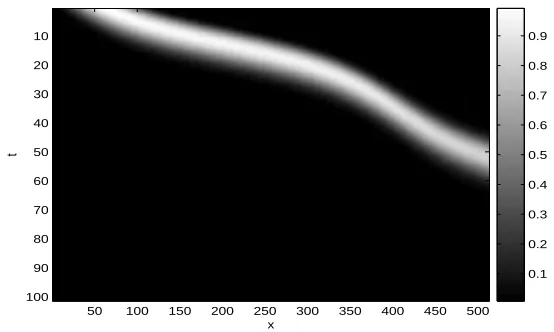
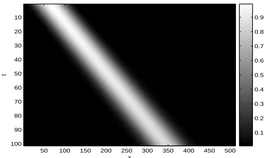
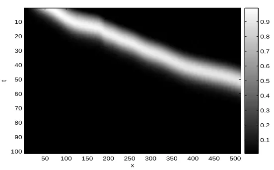
For the purpose of identification using the proposed approach, the PDE (23) with f(x, t) ≡ 0, were numerically solved for all three cases by a fourth-order Runge-Kutta method with a space step ∆x = 1/512. The data with a time length 1 and a time step ∆t = 0.01 are plotted in Figs.(1) to (3).

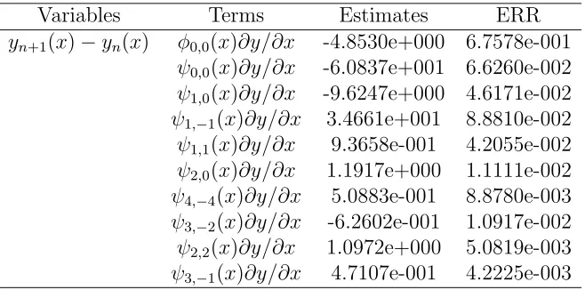
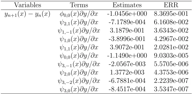
A set of 3000 spatio-temporal observations randomly selected out of 513×101 data points was used for the identification. In the simulation, the highest order of the derivatives with respect to the spatial variables was set to be 1. The 3rd Adams-Moulton integration formula was used and the polynomial expansion of order 2 was used. The order of B-spline was set to be 3, 3, 2, initial scale was 0, 0, 0, and the maximal resolution was 3, 4, 3 for the three cases, respectively. In order to obtain simple models, the number of final model terms was set to be 10. The identified terms and parameters using the orthogonal least squares algorithm for all the three cases are listed in Tables (1) to (3), where ERR denotes the Error Reduction Ratio. The corresponding approximated coefficient functions are

Case 1

˜

a(x) = 3.0446φ0,0(x) + 96.774ψ0,0(x)−63.173ψ1,−1(x) + 13.015ψ1,0(x) (27) −1.9225ψ1,1(x) + 0.62128ψ2,−3(x)−0.11742ψ2,−1(x) + 0.031824ψ2,0(x) −0.15484ψ2,2(x)−0.16752ψ3,2(x)

Case 2

˜

a(x) = 4.853φ0,0(x) + 60.837ψ0,0(x)−34.661ψ1,−1(x) + 9.6247ψ1,0(x) (28) −0.93658ψ1,1(x)−1.1917ψ2,0(x)−1.0972ψ2,2(x) + 0.62602ψ3,−2(x)

x

t

50 100 150 200 250 300 350 400 450 500

10 20 30 40 50 60 70 80 90 100

0.1 0.2 0.3 0.4 0.5 0.6 0.7 0.8 0.9

Figure 2: Data y(x, t) for case 2

x

t

50 100 150 200 250 300 350 400 450 500

10 20 30 40 50 60 70 80 90 100

0.1 0.2 0.3 0.4 0.5 0.6 0.7 0.8 0.9

Variables Terms Estimates ERR

yn+1(x)−yn(x) φ0,0(x)∂y/∂x -3.0446e+000 5.1278e-001

ψ0,0(x)∂y/∂x -9.6774e+001 1.3036e-001

ψ1,−1(x)∂y/∂x 6.3173e+001 1.2241e-001

ψ1,0(x)∂y/∂x -1.3015e+001 2.0299e-001

ψ1,1(x)∂y/∂x 1.9225e+000 3.0368e-002

ψ2,−1(x)∂y/∂x 1.1742e-001 6.0335e-004

ψ2,−3(x)∂y/∂x -6.2128e-001 1.0961e-004

ψ2,2(x)∂y/∂x 1.5484e-001 5.2546e-005

ψ2,0(x)∂y/∂x -3.1824e-002 1.4463e-005

ψ3,2(x)∂y/∂x 1.6753e-001 1.0272e-005

Table 1: The terms and parameters of the final model for case 1

Variables Terms Estimates ERR

yn+1(x)−yn(x) φ0,0(x)∂y/∂x -4.8530e+000 6.7578e-001

ψ0,0(x)∂y/∂x -6.0837e+001 6.6260e-002

ψ1,0(x)∂y/∂x -9.6247e+000 4.6171e-002

ψ1,−1(x)∂y/∂x 3.4661e+001 8.8810e-002

ψ1,1(x)∂y/∂x 9.3658e-001 4.2055e-002

ψ2,0(x)∂y/∂x 1.1917e+000 1.1111e-002

ψ4,−4(x)∂y/∂x 5.0883e-001 8.8780e-003

ψ3,−2(x)∂y/∂x -6.2602e-001 1.0917e-002

ψ2,2(x)∂y/∂x 1.0972e+000 5.0819e-003

ψ3,−1(x)∂y/∂x 4.7107e-001 4.2225e-003

Table 2: The terms and parameters of the final model for case 2

Case 3

˜

a(x) = 1.0456φ0,0(x) + 1.1490ψ0,0(x)−0.31879ψ1,−1(x) + 0.38996ψ1,0(x) (29) −0.39072ψ1,1(x)−0.0013772ψ2,0(x)−0.00071789ψ2,1(x) + 0.00067881ψ3,−2(x)

+0.0020567ψ3,−1(x) + 0.00084517ψ3,0(x)

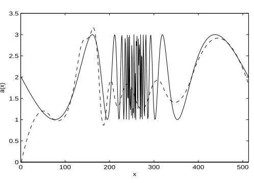
The identified coefficient function ˜a(x) and the original coefficient function a(x) are shown in Figs. (4) to (6) for the three cases. From (27), it can be observed that the wavelet components with low frequencies have large wavelet coefficients while the high frequency components have small coefficients (the coefficients are all less than 1.0 for all of the 22_{- and 2}3_{−components).}

Variables Terms Estimates ERR

yn+1(x)−yn(x) φ0,0(x)∂y/∂x -1.0456e+000 8.3695e-001

ψ2,1(x)∂y/∂x -7.1789e-004 6.1608e-002

ψ1,−1(x)∂y/∂x 3.1879e-001 3.6343e-002

ψ1,0(x)∂y/∂x -3.8996e-001 4.2967e-002

ψ1,1(x)∂y/∂x 3.9072e-001 2.0281e-002

ψ0,0(x)∂y/∂x -1.1490e+000 9.0303e-005

ψ3,−1(x)∂y/∂x -2.0567e-003 5.5705e-006

ψ2,0(x)∂y/∂x 1.3772e-003 4.3753e-006

ψ3,−2(x)∂y/∂x -6.7881e-004 2.2239e-007

ψ3,0(x)∂y/∂x -8.4517e-004 3.5347e-007

Table 3: The terms and parameters of the final model for case 3

that the signal is essentially nonlinear which is coincident with the property of the original signal a(x) = 2−sin(πtan(πx)). Moreover, it is interesting to notice from Fig.(5), for the fast oscillating part (in the middle of the plot) of a(x) the ˜a(x) look like a smoothed or averaged version of the original signal. This seems to indicate that the obtained PDE can be considered as a homogenisation of the original PDE, which represents the coarse behaviour of the underlying system. This happens for case 3 as well (see Fig. (6)) while note that since a(x) in this case is a random signal so that it is not possible to identify the signal itself. One of the reasons for this phenomenon may be from the selected approximation space for the a(x), which isV5 and V4 for

case 2 and case 3 while the frequency ranges of the orignal signal a(x) are 256 = 28_{Hz and ∞}

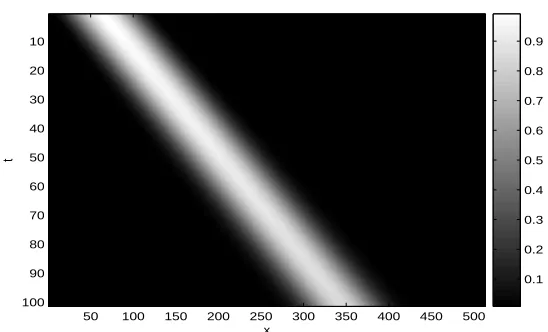
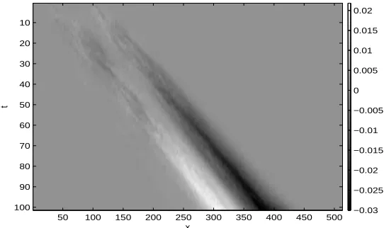
for case 2 and case 3, respectively. To further verify the identified results, the hyperbolic model equation (23) were numerically simulated using a fourth-order Runge-Kutta method again but with ˜a(x) for case 2 and case 3. The simulation results and the errors are plotted in Figs. (7) to (10), which show good performance for all two cases. Moreover, Figs. (8) and (10) show that the evolutions from the identified models are slightly slower than the original systems, which reflects the influence of the rapidly osillatory parameters on the behavior of the systems at an coarse scale.

5

Conclusions

0 100 200 300 400 500 0

0.5 1 1.5 2 2.5 3 3.5

x

a(x)

Figure 4: ˜a(x) (dashed) and a(x) (solid) for case 1

0 100 200 300 400 500

0 0.5 1 1.5 2 2.5 3 3.5

x

a(x)

0 100 200 300 400 500 0

0.1 0.2 0.3 0.4 0.5 0.6 0.7 0.8 0.9 1

x

a(x)

Figure 6: ˜a(x) (dashed) and a(x) (solid) for case 3

x

t

50 100 150 200 250 300 350 400 450 500

10 20 30 40 50 60 70 80 90 100

0.1 0.2 0.3 0.4 0.5 0.6 0.7 0.8 0.9

x

t

50 100 150 200 250 300 350 400 450 500

10 20 30 40 50 60 70 80 90 100

−0.2 −0.1 0 0.1 0.2 0.3

Figure 8: Error for case 2

x

t

50 100 150 200 250 300 350 400 450 500

10 20 30 40 50 60 70 80 90 100

0.1 0.2 0.3 0.4 0.5 0.6 0.7 0.8 0.9

x

t

50 100 150 200 250 300 350 400 450 500

10 20 30 40 50 60 70 80 90

100 _−0.03

−0.025 −0.02 −0.015 −0.01 −0.005 0 0.005 0.01 0.015 0.02

Figure 10: Error for case 3

6

Acknowledgement

The authors gratefully acknowledge financial support from EPSRC (UK).

References

[1] Basseville, M., Benveniste, A., Chou, K., Golden, S., Nikoukhah, R., and Willsky, S., (1992) Modelling and estimation of multiresolution stochastic processes, IEEE Trans. Inform. Theory, Vol. 38, pp. 766-784.

[2] Billings, S. A., Chen, S., and Kronenberg, M. J., (1988) Identification of MIMO nonlinear systems using a forward-regression orthogonal estimator, Int. J. Contr., Vol. 49, pp. 2157-2189.

[3] Billings, S A, and Coca D, (2002) Identification of coupled map lattice models of deterministic distributed parameter systems, Int J Systems Science, Vol. 33, pp. 623-34.

[4] Billings, S. A. and Coca, D., (2002a) Finite element Galerkin models and identified finite element models-a comparative study, 15th IFAC World Congress, Barcelona, Spain, pp. 2263-2268.

[5] Chen, S., Billings, S. A., and Luo, W., (1989) Orthogonal least squares methods and their application to non-linear system identification, International Journal of Control, Vol. 50, No. 5, pp. 1873-1896.

[7] Coca, D. and Billings, S. A., (2000) Direct parameter identification of distributed parameter systems, Int. J. Systems Sci., Vol. 31, No.1, pp. 11-17.

[8] Coca, D. and Billings, S. A., (2002b) Identification of finite dimensional models of infinite dimensional dynamical systems, Automatica, Vol. 38, pp. 1851-1856.

[9] Coca, D. and Billings, S. A., (2002c) Identification of finite dimensional models for distributed parameter systems, 15th IFAC World Congress, Barcelona, Spain, pp. 2256-2261.

[10] Daoudi, K., Frakt, A., and Willsky, S., (1999) Multiscale autoregressive models and wavelets, IEEE Trans. Inform. Theory, Vol. 45, No. 3, pp. 828-845.

[11] Digalakis, V.V. Chou, K.C., (1993), Maximum likelihood identification of multiscale stochastic models using the wavelet transform and the EM algorithm, Proceedings of 1993 IEEE International Conference on Acoustics, Speech, and Signal Processing, Vol. 4,pp. 93-96.

[12] E, W., Engquist, B., (2003) Multiscale modelling and computation, Notice of the AMS, Vol. 50, No. 9, pp.1062-1070.

[13] E, W., Engquist, B., Li, X., Ren, W., and Vanden-Eijnden, E., (2005) The heteroge-neous multiscale method: A review, http:// www.math. princeton. edu/ multiscale /review.pdf, pp.1-97.

[14] Fioretti, S. and Jetto, L., (1989) Accurate derivative estimation from noisy data: a state-space approach, Int. J. Systems Sci., Vol. 20, No. 1, pp.33-53.

[15] Guo, L. Z. and Billings, S. A., (2006), Identification of partial differential equation models for continuous spatio-temporal dynamical systems, IEEE Trans. Circuits & Systems-II: Express Briefs, Vol. 53, No. 8, pp. 657-661.

[16] Le, D. K., (1995) Multiscale system identification and estimation, Proceedings of

SPIE – Vol 2563: Advanced Signal Processing Algorithms, Franklin T. Luk, Editor,

pp. 470-481

[17] Mandelj, S., Grabec, I., and Govekar, E, (2001) Statistical approach to modeling of spatiotemporal dynamics, Int. J. Bifurcation & Chaos, Vol. 11, No. 11, pp. 2731-2738.

[18] Marcos-Nikolaus, P., Martin-Gonzalez, J. M. and S´ole, R. V., (2002) Spatial forcast-ing: detecting determinism from single snapshots, Int. J. Bifurcation and Chaos, Vol. 12, No. 2, pp. 369-376.

[19] Niedzwecki, J. M. and Liagre, P. -Y. F., (2003) System identification of distributed-parameter marine riser models, Ocean Engineering, Vol. 30, No. 11, pp. 1387-1415.

[21] Phillipson, G. A., (1971) Identification of distributed systems, American Elsevier, New York.

[22] Press, W. H., Flannery, B. P., Teukolsky, S. A., and Vetterling, W. T., (1992)

Numerical Recipes in FORTRAN: The Art of Scientific Computing, 2nd ed.

Cam-bridge, England: Cambridge University Press.

[23] Travis, C. C. and White, H. H., (1985) Parameter identification of distributed pa-rameter systems, Mathematical Bioscience, 77, pp. 341-352.

[24] Voss, H., Bunner, M. J., and Abel, M., (1998) Identification of continuous, spa-tiotemporal systems, Physical Review E, Vol. 57, No.3, pp. 2820-2823.