Abstract—As a recent approach for time series analysis, singular spectrum analysis (SSA) has been successfully applied for feature extraction in hyperspectral imaging (HSI), leading to increased accuracy in pixel-based classification tasks. However, one of the main drawbacks of conventional SSA in HSI is the extremely high computational complexity, where each pixel requires individual and complete singular value decomposition (SVD) analysis. To address this issue, a fast implementation of SSA (F-SSA) is proposed for efficient feature extraction in HSI. Rather than applying pixel-based SVD as conventional SSA does, the fast implementation only needs one SVD applied to a representative pixel, i.e. either the median or the mean spectral vector of the HSI hypercube. The result of SVD is employed as a unique transform matrix for all the pixels within the hypercube. As demonstrated in experiments using two well-known publicly available data sets, almost identical results are produced by the fast implementation in terms of accuracy of data classification, using the support vector machine (SVM) classifier. However, the overall computational complexity has been significantly reduced.
Index Terms—Data classification, fast singular spectrum analysis (F-SSA), feature extraction, hyperspectral imaging (HSI), support vector machine (SVM).
I. INTRODUCTION
ITH both spatial and spectral data simultaneously acquired forming a hypercube structure, hyperspectral imaging (HSI) has provided enhanced capabilities in data analysis and mining. Having spectral range covered from visible band to (near) infrared, HSI can be used in characterizing minor difference or changes among materials in terms of temperature, moisture and chemical components. As a result, HSI has been successfully applied in a number of emerging tasks such as food quality assessment, verification of faked documents and land-cover analysis in remote sensing [1-4].
Manuscript received July 30th 2014, revised October 15th 2014. Partial of the work is co-funded by National Nature Science Foundation of China under projects (#61202165, #61272381, #61003201) and an Exchange Project with Royal Society of Edinburgh (#6121130125).
J. Zabalza, J. Ren*, and S. Marshall are all with the Centre for excellence in Signal and Image Processing, Dept. of Electronic and Electrical Engineering, University of Strathclyde, Glasgow, U.K. (Emails: [email protected],
[email protected], [email protected], phone for corresponding author, Dr. J. Ren: +44-141-5482384).
Z. Wang is with School of Computer Software, Tianjin University, Tianjin, China (Email: [email protected]).
H. Zhao is with School of Electronics and Information, Guangdong Polytechnic Normal University, China (Email: [email protected]).
J. Wang is with School of Electronic and Information Engineering, Beijing Univ. of Aeronautics & Astronautics, China (Email: [email protected]).
In HSI, classification of the pixels from a scene can be accurate thanks to the dimension of features (spectral bands) provided, especially for powerful classifiers as support vector machine (SVM) [4-5]. Usually a feature extraction stage is implemented in the spectral domain prior to feeding the classifier. For feature extraction in HSI, projection based methods such as principal component analysis (PCA) [6] have been widely used, where several variations can also be found in [7-9]. Other well-known techniques include independent component analysis (ICA) [10], maximum noise fraction (MNF) [11] and nonnegative matrix factorization (NMF) [12-13]. Approaches for sparse representation of data [14-15] and spatial feature extraction [16-18] also become of interest in recent years.Nonetheless, since HSI data is prone to noise, it is encouraging the idea of a potential decomposition in the spectral domain of the pixels so noise can be avoided. Regarding this idea, an inspiring research for us is [19], where the empirical mode decomposition (EMD) technique applied in 1-D to the pixels is briefly evaluated for classification tasks.
Being part of the Hilbert Huang transform (HHT) for non-linear and non-stationary data analysis, EMD decomposes a 1-D signal into few components called intrinsic mode functions (IMFs) for a later reconstruction by only specific IMFs [20]. Although the reconstruction aim was to achieve higher accuracy in classification tasks, [19] showed deterioration. Unlike EMD, singular spectrum analysis (SSA) technique evaluated in a similar way is able to produce better results [21-22] as it enhances the spectral pixels, becoming a promising feature extraction technique in the HSI field.
However, in conventional SSA, pixel-based implementation of the SVD is required [21-22], which inevitably results in extremely high computational complexity in its implementation. To this end, a fast solution of SSA implementation in HSI is proposed in this paper, where SVD is only needed once. Actually, this unique SVD is applied to either the median or the mean spectral profile of the hypercube, whose results are then taken as a unique transform matrix for all the pixels in the hypercube. In this paper, we evaluate and compare the performance derived from PCA, ICA, MNF, and NMF with EMD, SSA and the fast implementation of SSA (F-SSA), where it is found that SSA surpass the rest of methods, and that F-SSA produces almost the same results as SSA, yet the computational complexity has been greatly improved.
The remaining parts of the paper are organized as follows. Section II describes the conventional SSA algorithm, with our proposed F-SSA discussed in Section III. Experiments and
Fast Implementation of Singular Spectrum
Analysis for Effective Feature Extraction
in Hyperspectral Imaging
J. Zabalza, J. Ren, member, IEEE, Z. Wang, H. Zhao, J. Wang and S. Marshall
results are discussed in Section IV, followed by some concluding remarks drawn in Section V.
II. CONVENTIONAL SINGULAR SPECTRUM ANALYSIS As a recent technique for time series analysis and forecasting, SSA [23] also allows interesting possibilities in other applications. SSA is able to decompose an original series into several independent components that are interpretable as varying trend, oscillations or noise. In fact, extractions of trends, periodic components or smoothing, as summarized in [23], are some of the main capabilities of SSA.
Given a 1-D signal defined as N
N
x x
x
[ 1, 2,, ]
x , the
SSA algorithm can be applied in the following steps. A. Embedding
Defining a window size LZ where L[1,N] , the trajectory matrix X of the vector x can be constructed as
K
N L L K K x x x x x x x x x C C C
X 1, 2, ,
1 1 3 2 2 1
. (1)
Columns of X are Ck[xk,xk1,xkL1]TL, lagged vectors where k[1,K] and KNL1. Matrix X has equal values in the anti-diagonals, i.e. is Hankel type.
Based on properties of the matrix X [23], SSA algorithm can be implemented symmetrically in two intervals, i.e.
)] 2 / ( , 1
[ round N
L and L[ceil((N1)/2),N]. For a given
L, the equivalent implementation can be found for another
K
L' , leading to the same results. B. Singular Value Decomposition
Defining a matrix S from the trajectory matrix X as
T
X X
S , the eigenvalues of S and their respective eigenvectors are then denoted respectively as
1
2
L
and
U1,U2,,UL
.The SVD of the matrix X is formulated below. Although the
d is equal to the rank of X, we consider dL for simplicity
d
X X
X
X 1 2 . (2)
Thus, the trajectory matrix X is actually built by the addition of several matrices Xi|i[1,d], which are called elementary
matrices, related to the respective eigenvalue as defined by
i i T i T i i i
i UV , V X U /
X . (3)
Matrices U and V are called matrix of empirical orthogonal functions and matrix of the principal components, respectively
K L L L L L V V V V U U U U , , , , , , 2 1 2 1 . (4)
C. Grouping
The total set of L individual components is now grouped into M disjoint sets denoted as I1,I2,,IM , where
Im L and m[1,M]. Let I
i1,i2,,ip
be one of the disjoint sets, the matrix XI related to I is then defined byip i
i
I X X X
X 1 2 . After the grouping, trajectory matrix X is represented as
IM I
I X X
X
X 1 2 . (5)
Please note that the basic grouping is the one with M L, and p1, where each set is made of just one component. D. Diagonal Averaging
After grouping, matrices XIm,m[1,M] obtained above are not necessarily Hankel type as the original trajectory matrix. Therefore, each one of these matrices needs to be hankelised (averaged in their anti-diagonals) for the projection into 1-D signals, as values in the anti-diagonals of each XIm contribute to the same element in the derived 1-D vector.
Denoting aj,nj1 as the elements of XIm , it can be projected to the 1-D signal zm[zm1,zm2,,zmN]N by
means of the diagonal averaging below
N n K a n N K n L a L L n a n z L K nj jn j
L
j jn j n
j jn j
mn
1, 1
1 , 1
1 , 1
1 1
1
1 1
. (6)
Finally, repeating this for every matrix XIm, the original 1-D signal x can be expressed as
M m m M 1 21 z z z
z
x , (7)
where the original signal can be reconstructed by using specific components, discarding those insignificant or prone to noise. E. SSA Application and Parameter Selection in HSI
formed by data embedding, thus can help to extract the local structures within the pixel vector.
SSA application in HSI is based on selecting some components and discarding the rest. As noisy artefact is usually located in the less significant eigenvalues, a reconstruction where these components are evaded, leads to enhanced spectral profiles and, therefore, better results. Hence, the feature enhancement provided by SSA is related to avoidance of noise. According to this fact, the next step is to determine what parameters use to avoid the noise. SSA application is governed by two parameters. The first is the window size L, which states the total number of components extracted in the decomposition stage. The second is the eigenvalue grouping (EVG), which denotes the selected combination of extracted components used for a desired reconstruction.
Selected parameters should ensure that reconstruction keeps the useful information of the spectral profiles while, at the same time, noisy content is discarded. As shown in [21], if EVG is small in relation to L, not only noise is removed but also some useful information (lossy region). On the opposite case, when EVG is large in relation to L, then some noise still remains in the reconstruction (noisy region). To this end, EVG must be related to L, so it would be appropriate to select EVG=1 for L=5 (or L=10), EVG=2 for L=20, or EVG=5 for L=40. This is further validated by the new results as reported in Section IV.D.
III. PROPOSED FAST SSA FOR HYPERSPECTRAL DATA ANALYSIS
Although SSA technique introduces added value to the data analysis by enhanced information extracted from the spectra, one remarkable drawback it has is the extremely high computational complexity required for pixel-based SVD. To address this problem, a fast implementation that requires only a single SVD is proposed as presented in detail below.
Our fast implementation of SSA is based on the common embedding process applied to every pixel before the SVD, which leads to similar transformation matrices so eventually a single matrix can be commonly applied to all the pixels. Moreover, this transformation matrix is obtained by a unique SVD that can be applied to a representative signal from the whole data set to be transformed.
A. F-SSA Concept
Conventional SSA application in HSI [21-22] works individually in each pixel. However, window size L in the embedding stage and components selected in the grouping stage are commonly applied to all the pixels. This fact allows our alternative F- SSA implementation.
As the embedding process is equal for all pixels, the assembly of lagged vectors and trajectory matrix structure is common for each individual case. As such, the orthonormal basis obtained from a unique SVD is able to transform the spectral profiles just in the same terms.
In addition, as all pixels in a hypercube are acquired by the same sensor under the same conditions, the distribution of general, system and/or environmental, noise tends to be
consistent (also other aspects, such as the water absorption regions location). Consequently, a set of eigenvectors can perfectly project the spectral profiles into reconstructed ones were noise is commonly avoided.
Regarding Eq. (2), the SVD of a signal results on different elements derived from the corresponding eigenvalues (or singular values). These elements Xi are dependent on Vi, both outputs from the SVD. However, according to Eq. (3), it is possible to substitute Vi in Xi, and therefore the elements from SVD can also be expressed in terms of inputted trajectory matrix and eigenvectors Ui as
X U U
Xi i Ti . (8)
In Eq. (8) we have just rearranged some basic SSA formulation so first, it is mathematically proved that F-SSA is feasible, and second, we can implement it in that manner. Consequently, any signal embedded with the adequate window
L in a trajectory matrix X can be transformed into several SSA components through some predefined eigenvectors. This key fact allows the use of a single set of eigenvectors to transform all pixels on a given data set.
B. Single SVD Analysis
[image:3.612.316.546.529.622.2]Since a unique set of eigenvectors can be employed to transform all Q pixels in a hypercube, an issue arises regarding which signal the single SVD has to be applied to. As the mean and the median computations over general sets of pixels have been intensively used in HSI related applications for feature extraction and data classification [24-25], these are employed here for obtaining the representative spectral profile of the data set, where it is simply computed as the average (or median) pixel from all those Q found in the hypercube (Fig. 1). In both cases, a unique pixel is introduced to represent the overall data set and this is considered to be an appropriate input to the SVD. Obviously, this input pixel needs to be embedded by the corresponding window L, same as the one requested in the analysis, leading to the representative trajectory matrix R.
Fig. 1. HSI hypercube with Q pixels (left) and the representative pixels (right) by the mean and the median computation from the whole hypercube.
C. Grouping
L p ipi i I
T I I I
U U U U
X U U X
, ,
, 2
1
. (9)
Therefore, after the SVD analysis, those eigenvectors selected for the reconstruction of the pixels are included in the columns of transformation matrix T
I IU
U .
D. Workflow of F-SSA
To highlight the difference between SSA and F-SSA, their workflows are illustrated in Fig. 2 for comparison. As can be seen, in F-SSA only the embedding, transformation and diagonal averaging procedures are required for all Q pixels, yet the transformation matrix derived from the representative pixel is commonly used to all of them. This can highly reduce the complexity of SSA when applied in HSI, as only an initial SVD analysis is demanded, which is carried out on a representative pixel, i.e. either the mean or the median spectral profile of the hypercube. The efficiency and efficacy of F-SSA are compared with SSA as detailed in the next section.
IV. EXPERIMENTS AND RESULTS
To evaluate both the conventional SSA and our proposed F-SSA, SVM-based data classification on two publicly available remote sensing data sets are used for comparison. A complete description of the data employed, experimental settings used and results achieved are detailed as follows. A. Data Description
Two remote sensing data sets with available ground truth for land-cover classification purposes are employed in our experiments. The first is the AVIRIS 92AV3C data set [26], which is a subscene acquired from Indiana, USA. With 145×145 pixels in 220 spectral reflectance bands, this data set contains elements in 16 labeled classes. The second is the ROSIS Pavia CA data set, a subscene extracted from a largest data set [27]. This was taken over Pavia, Northern Italy, made of 150×150 pixels and 102 spectral bands with elements labeled in a total of 7 classes. Spectral images with corresponding ground
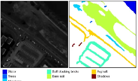
[image:4.612.94.518.49.231.2] [image:4.612.323.557.296.449.2]truth and elements to be classified are illustrated in Fig. 3 and Fig. 4, respectively.
Fig. 3. One band image at wavelength 667nm (left) and the ground truth maps (right) for the 92AV3C data set.
Fig. 4. One band image wavelength 521nm (left) and the ground truth maps (right) for the Pavia CA data set.
For data conditioning, as recommended by others [5, 19, 27], some bands are discarded, which results in the number of bands reduced from 220 to 200 and from 115 to 102, for the 92AV3C and Pavia CA data sets, respectively.
[image:4.612.322.557.497.636.2]B. Experimental Settings
Initially, the straight use of the original spectra from pixels is introduced as a Baseline reference for benchmarking. Then, several classical techniques such as PCA, ICA, MNF and NMF are also studied. After that, two main techniques, EMD and SSA, are evaluated for enhanced feature extraction and noise removal using reconstructed pixels in the HSI scene. Finally, our F-SSA proposal is implemented under same conditions for comparisons with conventional SSA.
In order to implement the classical techniques, MATLAB offers appropriate libraries for PCA, ICA and NMF, while for MNF we use an implementation based on Green’s method [11], where in all of them the main parameter is the dimension of features (f). For the decomposition techniques, on one hand we use the code available in [28] for EMD, adopting default (α) and experimentally determined (θ2=10×θ1) stop threshold values
[29], while in the reconstruction, combinations of the first, the first to second and the first to third IMFs are selected as suggested in [19]. On the other hand, for both SSA and F-SSA, several combinations of window L and EVG, as summarized in Table I, are selected to evaluate the corresponding performance.
TABLEI
FEATURE EXTRACTION METHODS AND PARAMETERS
Method Parameters Values adopted
Baseline N/A N/A
PCA
Dimension of features (f)
from 5 to original dimensionality in steps of 5 features (best one) ICA
MNF NMF
EMD Thresholds θ1, θ2, and α 0.8, 8, and 0.05 IMF grouping (IMFG) 1st, 1-2nd, 1-3rd
SSA / F-SSA EV grouping (EVG) Window size L 1st , 1-25, 10, 20, and 40 nd, 1-5th, 1-10th
Once the corresponding features are extracted, they are inputted to an SVM for data classification, as SVM is widely used in HSI [4-5] and remote sensing even in embedded systems [30-31]. LibSVM library [32] with Gaussian RBF kernel [4-5, 19] is used here, with penalty c and gamma γ parameters optimally determined through a grid search.
Every experiment is repeated ten times, varying the subsets for training and testing, in order to avoid systematic errors. Data partitions are randomly selected by stratified sampling, using an equal sample rate of 5% in each class for training. Finally, the mean results from classifying the testing partitions over the ten repetitions including McNemar’s tests [33] are reported.
Apart from the classification performance, we also compare the results from SSA and F-SSA in enhancing spectral profiles from pixels and evaluate their computational complexity. C. Enhancing Spectral Pixels with SSA and F-SSA
With both SSA and F-SSA, a spectral pixel in HSI can be reconstructed by selecting the main eigenvalue components, discarding those less representatives that usually contain noise and useless information. As stated in Section II.E, for data reconstruction two important parameters are needed in SSA: the window size L and the EVG (or selected components).
[image:5.612.337.536.124.276.2]For a given pixel-based spectral profile from 92AV3C data set, Fig. 5 illustrates the SSA reconstructed pixels using different EVG with L=10. As can be seen, the new profiles preserve the trend of the original signal but with potential reduction of noise.
Fig. 5. The original and reconstructed profiles by SSA for one pixel in HSI, with L=10 and EVG set as the 1st and the 1-5th eigenvalue component(s).
[image:5.612.336.536.380.532.2]Actually, the reconstructed spectral profile from F-SSA is almost the same as the one extracted from SSA. This has been clearly shown in Fig. 6, where almost identical results of reconstruction are produced using either the median or the mean spectral profile as the representative pixel.
Fig. 6. The original and reconstructed profiles using SSA and the two F-SSA schemes for one pixel in HSI, where L=10 and the EVG is set as the 1-5th eigenvalue components.
To take a closer look at the spectral profiles reconstructed from F-SSA and SSA, the relative difference │(xn-xn’)/xn│
between each reconstructed profile and the original profile is compared in Fig. 7. As can be seen, both SSA and the proposed F-SSA produce really similar profiles and result in same level of relative difference in comparison to the original profile.
several cases as shown in Table II. As can be seen, dissimilarity increases with the window size L, and decreases for larger EVGs. Nevertheless, in all cases, profiles from both the conventional SSA and proposed F-SSA are similar enough for a proper feature extraction in HSI.
Fig. 7. Relative difference (%) between the original profile and the ones reconstructed using SSA and the two F-SSA schemes, where L=10 and the EVG is set as the 1-5th eigenvalue components.
TABLEII
MEAN COSINE SIMILARITY SCORES TO QUANTIFY THE DIFFERENCE BETWEEN THE ORIGINAL AND RECONSTRUCTED PROFILES BY SSA AND F-SSAFROM THE
92AV3CDATA SET
Conventional SSA
L\EVG 1st 1-2nd 1-5th 1-10th
5 99.7514 99.9092 100 N/A 10 99.3228 99.7716 99.9367 100 20 98.4455 99.3706 99.8411 99.9408 40 97.5394 98.4087 99.5434 99.8438
F-SSA (mean)
L\EVG 1st 1-2nd 1-5th 1-10th
5 99.7513 99.9091 100 N/A 10 99.3228 99.7716 99.9365 100 20 98.4472 99.3732 99.8411 99.9410 40 97.5342 98.3275 99.5489 99.8433
F-SSA (median)
L\EVG 1st 1-2nd 1-5th 1-10th
5 99.7513 99.9091 100 N/A 10 99.3226 99.7716 99.9362 100 20 98.4469 99.3730 99.8411 99.9412 40 97.5356 98.3392 99.5506 99.8434
D. Results of Data Classification
For the two data sets 92AV3C and Pavia CA, the results of data classification are evaluated in this group of experiments. Features extracted from F-SSA are benchmarked with those from the Baseline, PCA, ICA, MNF, NMF, EMD [19-20] and conventional SSA [21-22] approaches. First of all, for the Baseline, classical techniques, and EMD, results of the mean overall accuracy (MOA) and mean McNemar’s test (MMT) are given in Table III, in comparison with those using SSA and F-SSA as given in Table IV and Table V.
As shown in Table III and Table IV, the Baseline approach has a MOA of 78% for the 92AV3C data set, and this has been improved to over 82% by using SSA or F-SSA, surpassing the
best case of the rest of methods evaluated. The classical methods provide limited accuracy in comparison with the SSA techniques and also present some other drawbacks; for instance, ICA and NMF are influenced by the initial values for iterations, and MNF is dependent on the algorithm to estimate the noise. Meanwhile, the SSA techniques are reliable, consistent and provide better classification accuracy.
TABLEIII
MEAN OVERALL ACCURACY (%) AND MEAN MCNEMAR’S TEST [Z] OF THE
BASELINE,PCA,ICA,MNF,NMF,EMD, AND SSAAPPROACHES
Method Parameters 92AV3C Pavia CA Baseline N/A 78.07 [-0.00] 97.10 [-0.00]
PCA f=15, and f=5 77.01 [-2.36] 97.06 [-0.15] ICA f=20, and f=5 76.90 [-2.61] 96.93 [-0.74] MNF f=10, and f=5 78.03 [-0.13] 97.16 [+0.12] NMF f=70, and f=10 78.58 [+1.28] 97.15 [+0.25]
EMD
IMFG=1st 48.33 [-47.2] 68.23 [-40.7] IMFG=1-2nd 52.28 [-41.8] 79.55 [-30.7] IMFG=1-3rd 65.40 [-24.2] 90.71 [-16.6] SSA L=10 EVG=1st 82.13 [+10.9] 97.35 [+1.19]
TABLEIV
MEAN OVERALL ACCURACY (%) AND MEAN MCNEMAR’S TEST [Z] FOR THE
92AV3CDATA SET USING SSA AND F-SSA Parameters SSA F-SSA
(mean)
F-SSA (median)
L EVG
5 1st 82.15 [+11.1] 82.12 [+11.2] 82.13 [+11.2] 5 1-2nd 80.68 [+7.58] 80.54 [+7.17] 80.54 [+7.16] 10 1st 82.13 [+10.9] 82.19 [+10.9] 82.17 [+11.0] 10 1-2nd 81.67 [+9.78] 81.94 [+10.8] 82.06 [+11.0] 10 1-5th 79.68 [+4.85] 79.85 [+5.50] 79.73 [+5.06] 20 1st 80.82 [+7.40] 80.86 [+7.44] 80.87 [+7.44] 20 1-2nd 82.15 [+10.9] 82.06 [+10.7] 82.05 [+10.5] 20 1-5th 81.67 [+9.86] 81.63 [+9.85] 81.49 [+9.51] 20 1-10th 79.13 [+3.29] 79.47 [+4.39] 79.47 [+4.38] 40 1st 79.46 [+3.74] 78.61 [+1.48] 78.61 [+1.47] 40 1-2nd 80.29 [+5.67] 80.64 [+6.90] 80.65 [+6.82] 40 1-5th 82.56 [+12.0] 82.19 [+11.1] 82.39 [+11.6] 40 1-10th 81.52 [+9.65] 81.14 [+8.58] 81.15 [+8.59] Overall mean 81.07 [+8.21] 81.02 [+8.15] 81.02 [+8.13]
TABLEV
MEAN OVERALL ACCURACY (%) AND MEAN MCNEMAR’S TEST [Z] FOR THE
PAVIA CADATA SET USING SSA AND F-SSA
Parameters
SSA (mean) F-SSA (median) F-SSA
L EVG
[image:6.612.319.562.333.527.2] [image:6.612.319.561.553.733.2]This, on one hand, has clearly indicated that SSA and F-SSA improves the discriminant ability of extracted features. In addition, as McNemar’s tests having Baseline as a reference show statistical significance at a confidence level of 95% when │Z│> 1.96, this also validates the improvement of SSA and F-SSA. On the other hand, it is found that F-SSA using either the mean or the median spectral profile of the hypercube yields almost the same results as those from SSA, where the overall mean value from all the configurations also proves the similarity in the results obtained from these three SSA approaches.
For the Pavia CA data set, similar findings can be observed from the associated results in Table III and Table V. Although MOA from the Baseline is already as high as 97.1%, SSA and F-SSA can still improve it to over 97.35%, where the two F-SSA schemes have generated almost the same results. Depending on the selected parameters, occasionally SSA and F-SSA slightly degrade MOA to 96.8% but in most cases they beat the other methods results.
TABLEVI
CLASS-BY-CLASS ACCURACIES (%) FOR THE 92AV3CDATA SET OBTAINED FROM THE BASELINE,SSA(L=10,EVG=1ST) AND F-SSA(L=10,EVG=1ST)
APPROACHES AS WELL AS THE NUMBER OF SAMPLES (NOS) IN EACH CLASS
Class NoS Baseline SSA (mean) F-SSA (median) F-SSA
54 37.84 75.29 75.29 74.71 1434 74.71 81.57 81.67 81.28 834 60.71 69.04 70.03 69.57 234 54.01 65.09 64.59 64.37 497 87.25 89.66 89.56 89.34 747 93.06 93.23 93.30 93.26 26 57.08 82.08 82.08 82.08 489 96.88 96.29 96.42 96.42 20 22.11 44.74 43.68 44.21 968 66.55 72.71 72.76 72.72 2468 81.19 82.92 82.94 83.19 614 68.70 81.87 82.35 82.18 212 95.27 96.22 96.07 96.12 1294 94.71 94.84 94.31 94.62 380 44.68 44.02 43.99 44.27 95 82.89 84.89 85.22 84.89 Average accuracy 69.85 78.40 78.39 78.33 Overall accuracy 78.07 82.13 82.19 82.17
TABLEVII
CLASS-BY-CLASS ACCURACIES (%) FOR THE PAVIA CADATA SET OBTAINED FROM THE BASELINE,SSA(L=10,EVG=1ST) AND F-SSA(L=10,EVG=1ST)
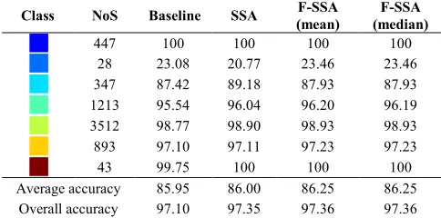
APPROACHES AS WELL AS THE NUMBER OF SAMPLES (NOS) IN EACH CLASS
Class NoS Baseline SSA F-SSA (mean)
F-SSA (median)
447 100 100 100 100
28 23.08 20.77 23.46 23.46 347 87.42 89.18 87.93 87.93 1213 95.54 96.04 96.20 96.19 3512 98.77 98.90 98.93 98.93 893 97.10 97.11 97.23 97.23 43 99.75 100 100 100 Average accuracy 85.95 86.00 86.25 86.25
Overall accuracy 97.10 97.35 97.36 97.36
Although the MOA and MMT measurements above have validated the effectiveness of SSA and F-SSA approaches in improved data classification, the class-by-class results are given in Table VI and Table VII for more detailed comparisons. For both 92AV3C and Pavia CA data sets, SSA and F-SSA clearly show as well a general increment in average and class-by-class accuracies.
E. Computational Complexity for SSA and F-SSA
Although the spectral profiles reconstructed from SSA and F-SSA are almost identical and produce similar results in data classification, the fast solution proposed in F-SSA is more efficient as analyzed in detail below.
As only a single SVD analysis is required in F-SSA, the saving factor in SVD stage is Q, i.e. the number of pixels in the given hypercube. Nevertheless, the saving factor for data embedding and diagonal averaging is still 1. For data grouping, although the transformation matrix needs to be computed only once, the overall saving factor remains closely to 1. This is because the unchanged grouping transformation part dominates the computational cost in this stage due to K p.
According to an introductory computational complexity analysis of the SSA algorithm in [35], step-wise complexity of the techniques presented in terms of multiplicate-accumulates (MACs) is given in Table VIII for comparisons. The embedding stage only consists of relocating the elements from a vector array into a matrix, so no MACs are involved. In relation to the second stage, even though SSA algorithm is normally formulated with the use of the SVD [23, 35], the SVD of the trajectory matrix X can be more easily implemented by an equivalent formulation applying eigenvalue decomposition (EVD) to SXXT, which is faster and more efficient than the
SVD complexity (L2KLK2K3) suggested in [35-36]. Accordingly, we use EVD for both methods applied to S.
The grouping stage is divided in two parts, referring first to EVG-based calculation of the single transformation matrix
T I IU
U and second to the transformation applied to every pixel. Finally, the diagonal averaging stage, although expressed in terms of multiplications and additions (N and LK for each pixel, respectively), can be approximated to a total number of
N MACs per pixel, where the final relocating process (from Hankel matrix to vector array) has no MACs associated, same as that in the first stage of data embedding.
TABLEVIII
COMPUTATIONAL COMPLEXITY (MACS) IN THE SSADIFFERENT STAGES
Stage SSA F-SSA Saving factor
Embedding - - 1
SVD [ L2K + L3 ] × Q [ L2K + L3 ] ×1 Q
Grouping Matrix UUT [L2p] × Q [ L2p ] ×1 Q Transformation [ L2K ] × Q [ L2K ] × Q 1 Diagonal Averaging [ N ] × Q [ N ] × Q 1
[image:7.612.51.293.603.723.2]analysis and transformation matrix obtainment. However, due to the cost for data transformation is at the same magnitude of pixel-based SVD, the overall saving factor becomes about 2.
For the two data sets 92AV3C and Pavia CA, the MACs required under different experimental settings are further compared in Table IX. In general, F-SSA has a saving factor of 2.0-2.7 in our experiments, which validates the analysis above. It is worth noting that the implementation of SVD without the optimized complexity, as suggested by Golub and Reinsch [35-36], results in much high computational cost of SVD. As a result, the cost for SVD stage is much higher than those for data transformation. To this end, the saving factor of F-SSA becomes significant, where the overall computational cost can be reduced to less than 5%.
TABLEIX
COMPUTATIONAL COMPLEXITY (MACS) FOR THE TWO DATA SETS IN
DIFFERENT CONFIGURATIONS (L=5,EVG=1ST),(L=40,EVG=1-10TH)
92AV3C Pavia CA
L= 5 40 5 40
EVG= 1st 1-10th 1st 1-10th
SSA 213e6 12.5e9 116e6 6.3e9 F-SSA 107e6 5.4e9 57e6 2.3e9 Saving factor 1.99 2.31 2.02 2.79
V. DISCUSSIONS AND CONCLUSIONS
Although SSA has been proved to be effective in feature extraction and data classification in HSI, it suffers from extremely high computational cost for pixel-based SVD analysis. By selecting a representation pixel using the median or the mean spectral profile of a given hypercube, a fast implementation of SSA, F-SSA, is proposed in determining the transformation matrix for data reconstruction.
It is found that the two F-SSA schemes actually produce almost the same reconstructed profiles as the conventional SSA does. Using the reconstructed profiles as features, these two F-SSA approaches are benchmarked with conventional SSA, EMD, classical techniques as PCA, ICA, MNF or NMF, and also the Baseline approach where the original spectral profiles are used. The results of SVM-based data classification validate the efficacy of the proposed F-SSA approaches. As only a unique SVD analysis is required in the proposed F-SSA, the overall computational cost has been significantly reduced.
Further research is ongoing for alternative implementations of the SSA techniques, where a particular approach with interesting potential can be the use of variable window sizes for object-oriented and saliency-based feature extraction [37-39].
REFERENCES
[1] T. Kelman, J. Ren, and S. Marshall, “Effective classification of Chinese tea samples in hyperspectral imaging,” Artificial Intelligence Research, 2(4): 87-96, 2013.
[2] J. Ren, S. Marshall, C. Craigie, and C. Maltin, “Quantitative assessment of beef quality with hyperspectral imaging using machine learning techniques,” 3rd Int. Conf. Hyperspectral Imaging, 2012.
[3] K. Gill, J. Ren, S. Marshall, S. Karthick, and J. Gilchrist, “Quality-assured fingerprint image enhancement and extraction using hyperspectral imaging,” 4th Int. Conf. Imaging for Crime Detection and Prevention, 2011.
[4] F. Melgani, and L. Bruzzone, “Classification of hyperspectral remote sensing images with support vector machines,” IEEE Transactions on Geoscience and Remote Sensing, 42(8): 1778–1790, August 2004. [5] R. Archibald, and G. Fann. “Feature selection and classification of
hyperspectral images with support vector machines.” IEEE Geoscience and Remote Sensing Letters, 4(4): 674-677, October 2007.
[6] I. Jlliffe, Principal Component Analysis. New York: Springer-Verlag, 1986.
[7] J. Ren, J. Zabalza, S. Marshall, and J. Zheng, “Effective feature extraction and data reduction in remote sensing using hyperspectral imaging,” IEEE Signal Processing Magazine, 31(4): 149-154, July 2014.
[8] J. Zabalza, J. Ren, M. Yang, Y. Zhang, J. Wang, S. Marshall, and J. Han, “Novel Folded-PCA for improved feature extraction and data reduction with hyperspectral imaging and SAR in remote sensing,” ISPRS Journal of Photogrammetry and Remote Sensing, 93:112-122, July 2014. [9] J. Zabalza, J. Ren, J. Ren, Z. Liu, and S. Marshall, “Structured covariance
principal component analysis for real-time onsite feature extraction and dimensionality reduction in hyperspectral imaging,” Applied Optics, 53(19): 4440-4449, July 2014.
[10] A. Hyvrinen, J. Karhunen, and E. Oja, Independent Component Analysis. New York: Wiley, 2001.
[11] A. A. Green, M. Berman, P. Switzer, and M. D. Craig, “A transformation for ordering multispectral data in terms of image quality with implications for noise removal,” IEEE Transactions on Geoscience and Remote Sensing, 26(1): 65-74, January 1988.
[12] S. A. Robila, and L. G. Maciak, “Sequential and parallel feature extraction in hyperspectral data using nonnegative matrix factorization,” IEEE Systems, Applications and Technology Conference, May 2007. [13] X. Huang, and L. Zhang, “An adaptive mean-shift analysis approach for
object extraction and classification from urban hyperspectral imagery,” IEEE Transactions on Geoscience and Remote Sensing, 46(12): 4173-4185, December 2008.
[14] C. Zhao, X. Li, J. Ren, and S. Marshall, “Improved sparse representation using adaptive spatial support for effective target detection in hyperspectral imagery,” Int. J. Remote Sensing, 34(24): 8669-84, 2013. [15] H. Zhang, J. Li, Y. Huang, and L. Zhang, “A nonlocal weighted joint
sparse representation classification method for hyperspectral imagery,” IEEE Journal of Selected Topics in Applied Earth Observations and Remote Sensing, 7(6): 2057-2066, June 2014.
[16] X. Huang, and L. Zhang, “A comparative study of spatial approaches for urban mapping using hyperspectral ROSIS images over Pavia City northern Italy,” International Journal of Remote Sensing, 30(12): 3205-3221, 2009.
[17] X. Huang, and L. Zhang, “An SVM ensemble approach combining spectral, structural, and semantic features for the classification of high-resolution remotely sensed imagery,” IEEE Transactions on Geoscience and Remote Sensing, 51(1): 257-272, January 2013. [18] H. Yuan, Y. Y. Tang, Y. Lu, L. Yang, and H. Luo, “Spectral-spatial
classification of hyperspectral image based on discriminant analysis,” IEEE Journal of Selected Topics in Applied Earth Observations and Remote Sensing, 7(6): 2035-2043, June 2014.
[19] B. Demir, and S. Ertürk, “Empirical mode decomposition of hyperspectral images for support vector machine classification,” IEEE Trans. on Geoscience and Remote Sensing, 48(11): 4071-4084, 2010. [20] N. E. Huang, Z. Shen, S. R. Long, M. C. Wu, H. H. Shih, Q. Zheng, N.-C.
Yen, C. C. Tung, and H. H. Liu, “The empirical mode decomposition and the Hilbert spectrum for nonlinear and non-stationary time series analysis”, Proceedings of the Royal Society Mar. 1998.
[21] J. Zabalza, J. Ren, Z. Wang, S. Marshall, and J. Wang, “Singular spectrum analysis for effective feature extraction in hyperspectral imaging,” IEEE Geoscience and Remote Sensing Letters, 11(11): 1886-1890, 2014.
[22] J. Zabalza, J. Ren, and S. Marshall, “Singular spectrum analysis for effective noise removal and improved data classification in hyperspectral imaging,” in Proc. WHISPERS, June 2014.
[23] N. Golyandina, and A. Zhigljavsky, Singular Spectrum Analysis for Time series, Springer, 2013.
[25] S. Piqueras, J. Burger, R. Tauler, and A. de Juan, “Relevant aspects of quantification and sample heterogeneity in hyperspectral image resolution,” Chemometrics and Intelligent Laboratory Systems, 117: 169-182, August 2012.
[26] Pursue's university multispec site: June 12, 1992 aviris image Indian Pine Test Site [Online]. Available:
https://engineering.purdue.edu/~biehl/MultiSpec/hyperspectral.html
[27] Hyperspectral Remote Sensing Scenes [Online]. Available:
http://www.ehu.es/ccwintco/index.php?title=Hyperspectral_Remote_Se nsing_Scenes
[28] G. Rilling. Matlab/C codes for EMD and EEMD with examples [Online]. Available: http://perso.ens-lyon.fr/patrick.flandrin/emd.html
[29] G. Rilling, P. Flandrin, and P. Gonçalvés. “On empirical mode decomposition and its algorithms.” IEEE-EURASIP Workshop on Nonlinear Signal and Image Processing NSIP, 3, 2003.
[30] J. Zabalza, J. Ren, C. Clemente, G. Di Caterina, and J. J. Soraghan, “Embedded SVM on TMS320C6713 for signal prediction in classification and regression applications,” in 5th European DSP Education and Research Conf., Amsterdam, Sept. 2012.
[31] J. Zabalza, C. Clemente, G. Di Caterina, J. Ren, J. J. Soraghan, and S. Marshal, “Robust pca micro-doppler classification using SVM on embedded systems,” IEEE Trans. Aerospace and Electronic Systems, 50(3), July 2014.
[32] C-C. Chang, and C-J. Lin, LIBSVM: library for support vector machines. [Online]. Available: http://www.csie.ntu.edu.tw/~cjlin/libsvm
[33] G. M. Foody, “Thematic map comparison: Evaluating the statistical significance of differences in classification accuracy,” Photogramm. Eng. Remote Sens., 70(5): 627–633, May 2004.
[34] F. van der Heiden, R. P. W. Duin, D. de Ridder, and D. M. J. Tax, Classification, Parameter Estimation and State Estimation: An Engineering Approach Using MATLAB. Chichester, U.K.: Wiley, 2004. [35] A. Korobeynikov, “Computation-and space-efficient implementation of
SSA,” arXiv preprint arXiv: 0911.4498, 2009.
[36] G. Golub, and C. Reinsch, “Singular value decomposition and least squares solutions,” Numer. Math. 14, 403-420, 1970.
[37] J. Han, P. Zhou, D. Zhang, G. Cheng, L. Guo, Z. Liu, S. Bu, and J. Wu, “Efficient, simultaneous detection of multi-class geospatial targets based on visual saliency modeling and discriminative learning of sparse coding,”ISPRS Journal of Photogrammetry and Remote Sensing, 89: 37-48, 2014.
[38] G. Cheng, J. Han, L. Guo, X. Qian, P. Zhou, X. Yao, and X. Hu, “Object detection in remote sensing images using a discriminatively trained mixture model,” ISPRS Journal of Photogrammetry and Remote Sensing, 11, 2013.
![TABLE MEAN OVERALL 92AV3CACCURACY DATA (%)SIV AND MEAN MCNEMAR’S TEST [Z] FOR THE ET USING SSA AND F-SSA](https://thumb-us.123doks.com/thumbv2/123dok_us/1620615.115148/6.612.319.561.553.733/table-mean-overall-caccuracy-data-mean-mcnemar-using.webp)