On the correct implementation of Fermi–Dirac statistics and electron trapping in
nonlinear electrostatic plane wave propagation in collisionless plasmas
Hans Schamel and Bengt Eliasson
Citation: Physics of Plasmas 23, 052114 (2016); doi: 10.1063/1.4949341
View online: http://dx.doi.org/10.1063/1.4949341
View Table of Contents: http://scitation.aip.org/content/aip/journal/pop/23/5?ver=pdfcov
Published by the AIP Publishing
Articles you may be interested in
How electronic dynamics with Pauli exclusion produces Fermi-Dirac statistics J. Chem. Phys. 142, 134113 (2015); 10.1063/1.4916822
Linear electrostatic waves in a three-component electron-positron-ion plasma Phys. Plasmas 21, 122119 (2014); 10.1063/1.4905067
Small amplitude nonlinear electrostatic waves in a collisional complex plasma with positively charged dust Phys. Plasmas 17, 102901 (2010); 10.1063/1.3482213
Nonlinear electromagnetic wave equations for superdense magnetized plasmas Phys. Plasmas 16, 072114 (2009); 10.1063/1.3184571
On the correct implementation of Fermi–Dirac statistics and electron
trapping in nonlinear electrostatic plane wave propagation in collisionless
plasmas
HansSchamel1,a)and BengtEliasson2,b)
1
Physikalisches Institut, Universit€at Bayreuth, D-95440 Bayreuth, Germany
2
SUPA, Physics Department, University of Strathclyde, John Anderson Building, Glasgow G4 0NG, Scotland, United Kingdom
(Received 17 March 2016; accepted 1 April 2016; published online 19 May 2016)
Quantum statistics and electron trapping have a decisive influence on the propagation characteristics of coherent stationary electrostatic waves. The description of these strictly nonlinear structures, which are of electron hole type and violate linear Vlasov theory due to the particle trapping at any excitation amplitude, is obtained by a correct reduction of the three-dimensional Fermi-Dirac distribution function to one dimension and by a proper incorporation of trapping. For small but finite amplitudes, the holes become of cnoidal wave type and the electron density is shown to be described by a/ðxÞ1=2rather than a /ðxÞexpansion, where/ðxÞis the electrostatic potential. The general coefficients are presented for a degenerate plasma as well as the quantum statistical analogue to these steady state coherent structures, including the shape of/ðxÞand the nonlinear dispersion relation, which describes their phase velocity.
VC 2016 Author(s). All article content, except where otherwise noted, is licensed under a Creative
Commons Attribution (CC BY) license (http://creativecommons.org/licenses/by/4.0/). [http://dx.doi.org/10.1063/1.4949341]
I. INTRODUCTION
Plasmas support a large number of nonlinear structures such as shocks, double layers, solitons, envelop solitons, and vortices. A particular class of nonlinear structures occurs due to particle trapping, where ions or electrons are trapped in the self-consistent potential wells in the plasma. Such struc-tures arise naturally in streaming instabilities or other not necessarily large amplitude perturbations. Typically, the trapping leads to excavated regions in the phase (velocity, coordinate) space, and hence, they are often referred to as ion and electron holes.1–7Electron and ion holes have been observed in the laboratory8–11 and by satellite observations in space.12–14At much smaller scales and in dense plasmas, the electron density is so high that quantum effects must be taken into account.15,16 The reason is that the inter-particle distance is small enough that the wave-functions of the elec-trons start to overlap, and Pauli’s exclusion principle dictates that two electrons, which are fermions, cannot occupy the same quantum state. This changes the equilibrium distribu-tion of the electrons from a Maxwell-Boltzmann distribudistribu-tion to a more general Fermi-Dirac (FD) distribution that takes into account electron degeneracy effects. In the limiting case of zero temperature, the equilibrium distribution for the Fermi gas is a flat-topped distribution in momentum space (or in velocity space for non-relativistic particles). At very small scales, there are also effects due to electron tunneling, and in this case, the dynamics of a single electron is described by the Schr€odinger or Pauli equation, and statisti-cal models are based on the Wigner equation. Some works have taken into account the first-order electron quantum
tunneling effects in the description of electron holes,17,18but in this paper, we will neglect these effects. We deal with the general framework of structures within the Vlasov-Poisson (VP) description for which Bernstein, Greene, and Kruskal (BGK)20presented the first mathematically correct solution. Physically, however, another method, the pseudo-potential method19 has proven preferential, as it is mathematically as general and correct but allows from the outset the selection of additional physically relevant solutions that are not possi-ble to obtain within BGK theory.20 Hence, our model is semi-classical in that it takes into account the modification of the equilibrium electron distribution function to a Fermi-Dirac distribution, while we consider structures large enough that electron tunneling effects can be neglected.
II. CONSERVED QUANTITIES AND REDUCTION OF DIMENSIONALITY
For pedagogic reasons, we here briefly review some ba-sic properties of the Vlasov-Poisson system which will be of importance in Sections III–VII. For brevity, we restrict the discussion to electrons, but the results are easily extended to include one or more ion species. The Vlasov equation
@tþv r þ
e me
r/ rv
fe¼0 (1)
describes the evolution of the electron distribution function
fein 3 spatial and 3 velocity dimensions, plus time, wheree
is the magnitude of the electron charge, and me is the
elec-tron mass. The electrostatic potential / is obtained from Poisson’s equation
r2/¼ e 0
ni
ð
fed3v
; (2)
a)[email protected] b)
where ni is assumed to be an immobile and homogeneous
neutralizing ion background density. Using that the Vlasov and Poisson equations are Galilei invariant, stationary waves in an inertial frame moving with the phase velocity of the wave can be obtained by setting the time-derivative to zero in Eq.(3), giving time-independent Vlasov equation
v r þ e
me
r/ rv
fe¼0: (3)
Solutions of Eq.(3)areconstantalong particle trajectories in ðr;vÞ space, given by E ¼mev2=2e/¼ constant, where
v2¼v2
xþv2yþv2z, and hence a solution can be expressed as
fe¼f0ðEÞ, wheref0ðEÞ is any function of one argument. (f0 can also be a multi-valued, as discussed below.) The con-served energyEis essentially due to reversal and translational symmetries of the Vlasov equation in time. Depending on the shape of the potential /, there may exist additional symme-tries leading to other conserved quantities. The most important case for our purposes is when/depends only one spatial vari-able, which we will take to be in thex-direction. In this case, there is a translational symmetry along theyandzdirections, which leads to that theyandzcomponents of the particle mo-mentum (and velocity) are conserved (vy¼constant and vz¼constant along the particle’s trajectory) and can be used
to eliminate these quantities inE, so that a “one-dimensional” conserved energy can be found, Ex¼mev2x=2e/
¼ constant. Hence, the solution of the time-independent Vlasov equation for this case can be writtenfe¼f0ðEx;vy;vzÞ,
wheref0is a function of three arguments. A last step to reduce the two velocity dimensions perpendicular to thexaxis is to integrate the distribution function as
fe1DðExÞ ¼
ð ð
f0ðEx;vy;vzÞdvydvz: (4)
This one-dimensional distribution function is a solution of the one-dimensional (1D) Vlasov equation
vx@xþ
e me
/ð Þx@vx
fe1Dðx;vxÞ ¼0; (5)
obtained by integrating Eq.(3)overvyandvz, and where/is
governed by the 1D Poisson equation
@
2/
@x2 ¼
e
0
ni
ð
fe1Ddvx
: (6)
If the potential instead has a rotational symmetry (spher-ical or cylindr(spher-ical), an additional conserved quantity toE is the angular momentum with respect to the rotation axis, which can be used to construct classes of time-independent solutions of the Vlasov equation.21 Various extensions including a constant external magnetic field can be found in Refs.22–24and relativistic effects in Refs.25and26.
III. GENERAL FORMULATION OF ELECTRON TRAPPING
Consider a collisionless plasma, in which the unper-turbed homogeneous electron distribution function isf~0ð~vÞ,
with an equilibrium number densityn0and an electron tem-perature Te. The plasma frequency xpe¼
ffiffiffiffiffiffiffiffiffiffiffiffiffiffiffiffiffiffiffiffi
n0e2=me0
p
, the thermal velocityvthe¼ ffiffiffiffiffiffiffiffiffiffiffiffiffiffiffiffiffikBT0=me
p
, and the Debye screening lengthkDe¼vthe=xpe will be used for normalization of the
dependent variables, here temporarily being denoted by tilde, into their dimensionless form through t¼xpe~t;x¼~x=kDe; v¼~v=vthe;/¼e/~=kBT0, andf0ðvÞ ¼ ðvthe=n0Þf~0ð~vÞ, which
we will use below.
Consider next the underlying 1D Vlasov-Poisson (VP) system(5) and(6), which is perturbed by a coherent plane wave structure/ðx;tÞ ¼/ðxv0tÞthat propagates with
ve-locity v0 in the lab frame. It is then constant in time in a frame moving with the wave. In this wave frame, the normal-ized Vlasov equation hence becomes
½v@xþ/ðxÞ@vfeðx;vÞ ¼0; (7)
where we, for brevity, have dropped the superscript “1D” on
feand have writtenvx¼v. For our purposes, we write the
so-lution of Eq.(7)as
feðx;vÞ ¼f0ðnÞhðÞ þftðnÞhðÞ; (8)
where¼v2=2/ðxÞis the single particle energy andhðxÞ
is the Heaviside step function. The separatrix, which divides the phase space into a trapped and untrapped particle region, is given by ¼0. The unperturbed distribution function is thereby extended, as a consequence of/ðxÞ, to the inhomo-geneous distribution f0ðnÞ, which represents the untrapped
(or free) particles. The new argumentnis a generalized ve-locity27and is defined by
n¼hðÞsgnðvÞp2ffiffiffiffiffiþhðÞpffiffiffiffiffiffiffiffiffi2: (9)
The solution involves a two-parametric (sgnðvÞ,) constant of motion of (7), such that (8) solves (7). Note that n¼v
when/¼0 and that sgnðvÞis a constant of motion only for the untrapped particles. Hence, for >0,f0becomes multi-valued with respect toand depends also on sgnðvÞ. In Eq.
(8),ftðnÞrepresents the trapped electron distribution, which
is restricted to the trapped region,pffiffiffiffiffiffi2/vpffiffiffiffiffiffi2/, corre-sponding to 0. Here, we already have adopted a non-negative/. The electron density is thus obtained as
neð/Þ ¼
ð1
1
fedv¼
ðpffiffiffiffi2/
1
f0ð
ffiffiffiffiffi 2 p
Þdv
þ ð ffiffiffiffip2/
pffiffiffiffi2/
ftð
ffiffiffiffiffiffiffiffiffi
2
p
Þdvþ ð1
ffiffiffiffi
2/ p f0ð
ffiffiffiffiffi 2 p
Þdv: (10)
IV. HALF-POWER EXPANSION OF THE ELECTRON DENSITY
assumption that feðx;vÞ is continuous across the separatrix
and thatftðnÞis an analytic function innthat
neð Þ ¼/ 1þ
k2 0w
2 þa/þb/ 3 2þc/
2
2 þ ; (11)
wherek0will later be a measure of the wave’s wavenumber, and the coefficients are
a¼ P ð1
v@vf0ð Þv dv; (12)
b¼2
5=2
3 @
2
vf0jv¼0þ@ 2
nftjn¼0
; (13)
and
c¼ P ð 1
v@v
2
f0ð Þvdv; (14)
wherePdenotes the principal value. In(12)–(14), we made use of v¼n when /¼0, which is valid for untrapped electrons.
Deviations from continuity and analyticity have recently been treated in Ref.29. The coefficientcin Eq.(14)is given for completeness only and will not be used below. Trapping is manifested by theb/3=2term in Eq.(11). Equation(11)is hence a half-powerexpansion in/, in which the /1=2 term vanishes due to continuity at ¼0.29 This provides the for-mal background under which a wide range of collisionless plasmas can be treated formally on the same footing.
V. THE MAXWELLIAN CASE
We start with the general degenerated state and perform subsequently the classical Maxwellian limit, as follows. For fermions in a degenerate state, the unperturbed single parti-cle distribution is given by the Fermi–Dirac (FD) distribu-tion, which in the three-dimensional (3D) velocity space reads in dimensional units30
~
FFDð Þ ¼E~ 2m
3
e
h3
1
eðE~~lÞ=kBT0þ1
; (15)
where ~l is the chemical potential and E~¼ ð~v2xþ~v
2
y
þ~v2zÞ=2¼~v2=2 is the single particle energy in the 3D veloc-ity space (in lab frame). In the limit T0!0, one obtains
~
l¼~eF¼ ðh2=8meÞð3n0=pÞ 2=3
, which is the Fermi energy andhis Planck’s constant.
Returning to dimensionless quantities, we can hence write
FFDð Þ ¼E 1
A eð Elþ1Þ; (16)
where the normalization constant A¼n0h3=½2ðmekBT0Þ3=2
is proportional to n0. Moreover, l is now the normalized chemical potential and E¼ ðv2
xþv
2
yþv
2
zÞ=2¼v
2=2 is the
normalized single particle energy in the 3D velocity space (in the lab frame). Assuming a unit equilibrium density, the
relation betweenlandAis found by a 3D velocity integra-tion using spherical coordinates in velocity space
A¼ ð2pÞ3=2Li3=2ðelÞ; (17)
where
Linð Þ ¼z
X1
k¼1
zk
kn; jzj<1 (18)
is the polylogarithm function with indexn. By a 2D velocity integration overðvy;vzÞ-space, using cylindrical coordinates, we get the reduced, 1D distribution in the lab frame
f0FDð Þ ¼vx
ð ð
FFDð ÞE dvydvz¼2p
A ln 1þe
v2 x=2þl
: (19)
The Maxwellian case is formally (for more details, see later) obtained in the limit l! 1, which by the small value expansion LiðxÞ x gives A! ð2pÞ3=2el, which together with lnð1þev2
x=2þlÞ !ev2x=2þl give the Maxwellian distribution
f0Mð Þ ¼vx 1ffiffiffiffiffiffi 2p
p ev2x=2: (20)
The free particle distribution function in the wave frame, introducingv¼vxv0, then reads
f0ð Þ ¼v
1 ffiffiffiffiffiffi 2p
p eðvþv0Þ2=2: (21)
For the trapped particles, we use
ftð Þ ¼n
ev20=2 ffiffiffiffiffiffi 2p
p 1þb
2n
2
: (22)
Note that continuity at the separatrix wheren¼0 for fi-nite/is automatically guaranteed by Eqs.(21)and(22), and that(22)uses the lowest order terms of the Taylor expansion ofebj/¼0. This latter exponential expression was used
ear-lier for finite amplitude waves, e.g., in Refs.1–3and19, but the results are the same as long as w1. Insertion of expressions (21) and (22) into Eqs. (12) and (13), respec-tively, then yields
a¼aM
1 2Z
0
r v0=
ffiffiffi 2 p
; (23)
and
b¼bM¼
4 1bv2 0
3pffiffiffip e v2
0=2¼:4
3bðb;v0Þ; (24)
with
Zrð Þ ¼u
1 ffiffiffi p p P
ð expðt2Þ
tu dt; (25)
Zr0ð Þ ¼ u
2 ffiffiffi p p P
ðtexpðt2Þ
which are familiar expressions found in many earlier papers of Schamel and coworkers. We note again that theb -depend-ence offtand ofbMis a crucial ingredient of getting suited
trapped particle equilibria. If, as done by Landau and Lifshitz,31bis assumed zero, corresponding to a completely flat trapped particle distribution, then no solitary electron holes would exist theoretically,1 to give an example of its limited application (besides its restriction to v0¼0). The
hollow nature of the trapped particle vortices found in phase space, being a general feature of all numerically observed phase space structures, demands the incorporation of a b<0. The question is now how in a quantum statistical set-ting the corresponding structural equilibria turn out to be.
VI. THE FERMI–DIRAC CASE
For fermions in a degenerate state, we got (16) as the dimensionless Fermi-Dirac distributionFFDðEÞin 3D veloc-ity space, from which the reduced 1D distributionfFD
0 ðvxÞin
the lab frame(19)was obtained.
The reduced free particle distribution function for 0 in the wave frame, introducingv¼vxv0, then reads
f0FDð Þ ¼v
2p
A ln 1þe
ðvþv0Þ2=2þl: (27)
For the trapped particle distribution with <0, we choose the same function as in the Maxwellian case but with a dif-ferent factor that accounts for continuity at ¼0 (and at n¼0)
ftFDð Þ ¼n
2p
A ln 1þe
v2 0=2þl
1þb 2n
2
: (28)
Equations(27)and(28)are the two desired functions needed to deriveaandbfor the density expression (11)in the FD case. By insertion of(27)into(12), we first get
a¼aFDð Þ v0
1 2Z
l
r0 v0=
ffiffiffi 2 p
; (29)
where we defined the Fermi-Dirac plasma dispersion function
Zrlð Þ u
23=2p
A P
ðln 1 þelt2
tu dt; (30)
which is by definition real valued and whose derivative is given by
Zrl0ð Þ ¼ u
25=2p
A P
ð
t
1þet2l
ð ÞðtuÞdt: (31)
The generalized complex plasma dispersion function ZlðuÞ with a complex argumentuwould then be a one in which the principal value is replaced by the Landau contour.
We note thatZl
rðuÞ !ZrðuÞandZlr0ðuÞ !Zr0ðuÞin the
classical limitl 1. In the case of a standing wave pat-tern,v0 ¼0;aFD can be obtained by a direct integration and
can be expressed in terms of a polylogarithm function as
aFDð Þ ¼ 0
2p ð Þ3=2
A Li1=2 e
l
ð Þ: (32)
The function Li1=2ðxÞ is real-valued and negative for x<0.
On the other hand, for high phase velocitiesv01, we have
the asymptotic expansion
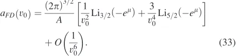
aFDð Þ ¼v0
2p ð Þ3=2
A
1
v2 0
Li3=2ðelÞ þ
3
v4 0
Li5=2ðelÞ
þO 1
v6 0
: (33)
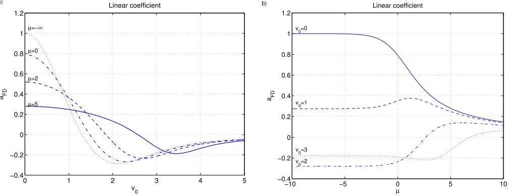
Figure1shows line-plots ofaFDðv0Þgiven by(29)for
differ-ent values ofv0andl. WhileaFDðv0Þis a decreasing
func-tion oflforv0¼0, the dependence ofaFDðv0Þonlis more
complicated for larger values ofv0with either local maxima or minima (cf. Fig.1(b)).
To obtainbFD, the two functionsf0FDðvÞandf
FD
t ðvÞhave
to be differentiated twice and, according to (13), the result has to be evaluated at v¼0 and n¼0, respectively. After some algebra, we get
b¼bFDð Þ v0
27=2p 3A
r v2
01r
1þr
ð Þ2 þbln 1ð þrÞ
" #
; (34)
where we definedr¼elv20=2. For a wave with zero velocity with respect to the lab frame, v0¼0, we hence get with
r0 ¼el
bFDð Þ ¼0
27=2p 3A
r0
1þr0
þbln 1ð þr0Þ
; (35)
a relative simple expression, which stands for the electron trapping nonlinearity in case of a non-propagating wave pat-tern in a degenerate plasma. The dependence ofbFDðv0Þon
v0,l, andbis shown in Fig.2.
VII. CNOIDAL ELECTRON HOLES AND THEIR SPEED
To close the system, i.e., to find self-consistent solutions for both systems, we have to solve the second part, the Poisson equation, which in the immobile ion limit becomes
/00ðxÞ ¼ ð
fðx;vÞdv1¼ V0ð/Þ: (36)
In the second step, we have introduced the pseudo-potential Vð/Þ. Its knowledge allows by a quadrature to find the final shape of the potential structure/ðxÞvia the pseudo-energy
1 2/
0
x
ð Þ2þ Vð Þ ¼/ 0; (37)
where we without loss of generality have assumedVð0Þ ¼0. Insertion of the electron density(11)into Eq.(36)and a subsequent/-integration yield
Vð Þ ¼/ k
2 0
2w/þ 1 2a/
2þ2
5b/
5=2þ : (38)
[image:5.607.324.559.141.197.2]The speed of the potential structure is obtained from the non-linear dispersion relation (NDR),VðwÞ ¼0, which becomes
k20þaþ
4b
5 ffiffiffiffi w p
þ:::¼0: (39)
Eliminatingain Eq.(38)by Eq.(39)we get
Vð Þ ¼/ k
2 0
2/ wð /Þ 2b
5 /
2 ffiffiffiffi
w p
pffiffiffiffi/
þ:::: (40)
It represents a typical cnoidal wave solution, a one being rep-resented by Jacobian elliptic functions such as cnðxÞ or snðxÞ. The first term in (40) represents a purely harmonic wave, and the second one is a solitary wave, provided that
b<0. The general two-parametric solution, which involves both terms, has been analyzed in Refs.32and33. It is a peri-odic function with an in general high content of Fourier har-monics. As said before, its phase velocity v0 is determined by the NDR(39).
In case of a Maxwellian unperturbed plasma, where we have to replace (a;b) by (aM; bM), the NDR can be written
as6,27–29,32,33
k20
1 2Z
0
r v0=
ffiffiffi 2 p
¼ 4 5bM
ffiffiffiffi w p
16
15bðb;v0Þ ffiffiffiffi w p
; (41)
where we used(24)in the last step to show coincidence with the previous result. In the more general degenerate electron state, we replace (a;b) by (aFD;bFD) in Eq. (39) to obtain
the NDR
k02
1 2Z
l
r0 v0=
ffiffiffi 2 p
¼ 4 5bFDð Þv0
ffiffiffiffi w p
; (42)
withbFDðv0Þgiven by (34).
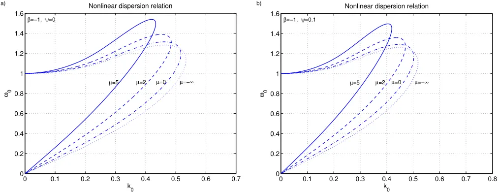
Figure 3shows plots of the NDR (42), where we used x0¼k0v0, for b¼ 1 and different values of l. Both the
[image:6.607.54.558.60.255.2] [image:6.607.54.556.545.744.2]zero amplitude limit w’0þ in Fig.3(a)and the small am-plitude casew¼0:1 in Fig.3(b)show similar features with FIG. 1. The linear coefficientaFDfor different values ofv0andl. Note thataFD!aMin the classical limitl 1.
the typical thumb shape of the dispersion curves in the (x0,
k0) space. In general, the wave frequency increases with increasing values ofl. The high-frequency Langmuir branch takes the frequencyx0!1 ask0!0 as can also be shown
by using the NDR (39)together with the asymptotic expan-sion(33)for a¼aFDtogether with Eq.(17)for A, and that
b¼bFD!0 in the limitv0! 1.
We note that the character of the dispersion relation changes and becomes “non-dispersive” with a lower cut-off fork0in the high frequency branch when the right hand side of the NDR is fixed rather than bandw(see Fig. 5 of Ref.
33). In case of a Maxwellian plasma, denoting the right hand side of(41) byBM, this cut-off is given byk^0:¼ ffiffiffiffiffiffiffiBM
p and
the phase velocity v0diverges as v20k21
0BM ask0!
^
kþ0. A
fixed BM then corresponds to a b¼ 15
ffiffi p p
16pffiffiffiwBMexpðv
2 0=2Þ,
which assumes extremely large negative values. In such a situation, the trapped electron range is more or less empty.
VIII. CONCLUSION
In conclusion, we have presented a general framework of weak coherent structures in partially Fermi-Dirac degen-erate plasmas. These coherent structures are necessarily determined by the electron trapping nonlinearity and hence are beyond any realm of linear Vlasov theory. This implies that even in the infinitesimal amplitude limit, linear Landau and/or van Kampen theory fail as possible descriptive approaches to these structures.29,33The spatial profiles of the potential /ðxÞ in the small amplitude limit are of cnoidal hole character, similar is in the classical case, and are given by the already known expressions (see Ref.33 and referen-ces therein). The NDR on the other hand is for given b;w again of thumb shape type but appears to be rather sensitive to the electron degeneracy characterized by the normalized chemical potential l. An important aspect of the nonlinear theory in the small but finite amplitude limit is that the elec-tron density is described by half-power expansions of the electrostatic potential. Different results34 not giving rise to
half-power expansions of the potential, which we find ques-tionable, are found by not following the recipe of first defin-ing trapped and free populations of electrons before calculating the electron density and by an incorrect reduction in the distribution function from 3D to 1D.
Finally, a mention on the validity of the present approach is necessary. We note that hot and non-degenerate plasmas are characterized by knkdB, wherekn ¼ ð4pn0=3Þ
1=3
is the mean particle distance andkdB ¼h=ðmevtheÞis the
ther-mal de Broglie wavelength with the reduced Planck’s con-stant h¼h=ð2pÞ, while cold and degenerate plasmas are characterized byknⱗkdB. In the latter limit, the equilibrium
distribution changes from a Maxwell-Boltzmann distribution to a Fermi-Dirac distribution. Moreover, the collisionless na-ture of the plasma requires that the mean kinetic energy of the particles is much larger than the mean potential energy due to Coulomb interactions between the particles. For a Maxwell-Boltzmann distributed plasma, this leads to the requirement 3kBT=2>e2kn=ð4p0Þ, or kn<kDe, while in
the cold limit of Fermi-Dirac distributed electrons, we have 3EFe=5>e2kn=ð4p0Þ, which is fulfilled for sufficiently
high densities n0ⲏa03 where a0¼4p0h2=ðmee2Þ 5:3
1011m is the Bohr radius, giving n0ⲏ6:31030m3.
This is larger than typical densities of conduction electrons in metals, 51028m3, but this restriction may be relaxed
due to Pauli blocking reducing the collisionality of the elec-trons.35,36 The use of the Vlasov approach against the more general Wigner framework of quasi-distributions6 necessi-tates the semi-classical limitDxDvh=me, whereDxis the
spatial length-scale of the structure and Dv is the velocity scale. As an example, ifDx1=k0is the typical length-scale
of a periodic wave-train and the velocity scale in an ultra-cold plasma is the Fermi speedDvvFe¼ ffiffiffiffiffiffiffiffiffiffiffiffiffiffiffiffi2EF=me
p
, then the Wigner approach has to be used when the wavelength k¼2p=k0 is small enough to be comparable to the
inter-particle distancekn. If the velocity scale is instead given by
the thermal speed vthein a warm, Maxwellian plasma, then
[image:7.607.51.558.58.253.2]the Wigner approach would only be necessary at extremely short wavelengths when k is comparable to kdBkn. The FIG. 3. The nonlinear dispersion relation (NDR) for (a)w¼0þand (b)w¼0:1, and different values oflwithb¼ 1, usingx0¼v0k0. The classical, non-degenerate case corresponds tol¼ 1.
Maxwellian limitl! 1is only a formal one, since rela-tivistic effects have to be taken into account when kBT
becomes comparable to the electron rest mass energymec2,
which occurs at temperatures higher than 109K, and in which case relativistic effects have to be taken into account in the treatment of electron holes.25 A similar constraint applies to very high densities when the electron Fermi energy
EF becomes comparable to mec2, which happens when the
knⲏkC, where kC¼h=ðmecÞ is the Compton wavelength;
this happens at densities n0ⲏ1034m3 that exist in dense
astrophysical bodies such as white dwarf stars.37,38
Planned future extensions of the theory are to take the above mentioned relativistic effects into account. A detailed examination of the NDR(42)is also delegated to a forthcom-ing paper where analytic expressions will be presented for the ldependence of the Langmuir branch, x01;k0 1,
and the slow electron acoustic branch x0/k0;k01. As
Fig. 3 shows, the slow branch is especially sensitive to l. Another extension is the replacement of the phase velocity
v0 by ~vD:¼vDv0, where vD is the drift velocity, in the
above expressions to handle a current in the electronic system.6,32,39,40
ACKNOWLEDGMENTS
B.E. acknowledges the support from the Engineering and Physical Sciences Research Council (EPSRC), UK, Grant No. EP/M009386/1. No data are associated with this article.
1H. Schamel, “Theory of electron holes,”Phys. Scr.20, 336 (1979). 2S. Bujarbarua and H. Schamel, “Theory of finite-amplitude electron and
ion holes,”J. Plasma Phys.25, 515 (1981).
3
H. Schamel, “Electron holes, ion holes and double layers,”Phys. Rep.
140, 161 (1986).
4B. Eliasson and P. K. Shukla, “Dynamics of electron holes in an
electron-oxygen-ion plasma,”Phys. Rev. Lett.93, 045001 (2004).
5
B. Eliasson and P. K. Shukla, “Production of non-isothermal electrons and Langmuir waves because of colliding ion holes and trapping of plasmons in an ion hole,”Phys. Rev. Lett.92, 095006 (2004).
6
A. Luque and H. Schamel, “Electrostatic trapping as a key to the dynamics of plasmas, fluids and other collective systems,”Phys. Rep.415, 261 (2005).
7B. Eliasson and P. K. Shukla, “Formation and dynamics of coherent structures
involving phase-space vortices in plasmas,”Phys. Rep.422, 225–290 (2006).
8K. Saeki, P. Michelsen, H. L. P
ecseli, and J. J. Rasmussen, “Formation and coalescence of electron solitary holes,”Phys. Rev. Lett.42, 501–504 (1979).
9G. Petraconi and H. S. Maciel, “Formation of electrostatic double-layers
and electron holes in a low pressure mercury plasma column,”J. Phys. D: Appl. Phys.36, 2798–2805 (2003).
10H. L. Pecseli, J. Trulsen, and R. J. Armstrong, “Experimental observation
of ion phase-space vortices,”Phys. Lett. A81, 386–390 (1981).
11H. L. P
ecseli, J. Trulsen, and R. J. Armstrong, “Formation of ion phase-space vortices,”Phys. Scr.29, 241–253 (1984).
12J. F. Drake, M. Swisdak, C. Cattell, M. A. Shay, B. N. Rogers, and A.
Zeiler, “Formation of electron holes and particle energization during mag-netic reconnection,”Science299, 873–877 (2003).
13
C. Cattell, J. Domebeck, J. Wygant, J. F. Drake, M. Swisdak, M. L. Goldstein, W. Keith, A. Fazakerley, M. Andr, E. Lucek, and A. Balogh,
“Cluster observations of electron holes in association with magnetotail reconnection and comparison to simulations,” J. Geophys. Res. 110, A01211, doi:10.1029/2004JA010519 (2005).
14J. P. McFadden, C. W. Carlson, R. E. Ergun, F. S. Mozer, L. Muschietti, I.
Roth, and E. Moebius, “FAST observations of ion solitary waves,”
J. Geophys. Res.108, 8018, doi:10.1029/2002JA009485 (2003).
15
P. K. Shukla and B. Eliasson, “Nonlinear aspects of quantum plasma phys-ics,”Phys. -Usp.53, 51–76 (2010).
16
P. K. Shukla and B. Eliasson, “Nonlinear collective interactions in quan-tum plasmas with degenerate electron fluids,” Rev. Mod. Phys. 83, 885–906 (2011).
17A. Luque, H. Schamel, and R. Fedele, “Quantum corrected electron
holes,”Phys. Lett. A324, 185–192 (2004).
18
D. Jovanovic´ and R. Fedele, “Coupling between nonlinear Langmuir waves and electron holes in quantum plasmas,” Phys. Lett. A 364, 304–312 (2007).
19
H. Schamel, “Stationary solitary, snoidal and sinusoidal ion acoustic waves,”Plasma Phys.14, 905 (1972).
20
I. B. Bernstein, J. M. Greene, and M. D. Kruskal, “Exact nonlinear plasma oscillations,”Phys. Rev.108, 546 (1957).
21
C. S. Ng and A. Bhattacharjee, “Bernstein-Greene-Kruskal modes in a three-dimensional plasma,”Phys. Rev. Lett.95, 245004 (2005).
22B. Eliasson and P. K. Shukla, “Localized kinetic structures in magnetized
plasmas,”Phys. Scr.T113, 38 (2004).
23C. S. Ng, A. Bhattacharjee, and F. Skiff, “Weakly collisional Landau
damping and three-dimensional Bernstein-Greene-Kruskal modes: New results on old problems,”Phys. Plasmas13, 055903 (2006).
24
B. Eliasson and P. K. Shukla, “Theory for two-dimensional electron and ion Bernstein-Greene-Kruskal modes in a magnetized plasma,”J. Plasma Phys.73(5), 715 (2007).
25
B. Eliasson and P. K. Shukla, “Theory of relativistic electron holes in hot plasmas,”Phys. Lett. A340(1–4), 237–242 (2005).
26
P. K. Shukla and B. Eliasson, “Localization of intense electromagnetic waves in a relativistically hot plasma,” Phys. Rev. Lett. 94, 065002 (2005).
27H. Schamel, “Analytic BGK modes and their modulational instability,”
J. Plasma Phys.13, 139 (1975).
28
J. Korn and H. Schamel, “Electron holes and their role in the dynamics of current-carrying weakly collisional plasmas. Part 1. Immobile ions,”
J. Plasma Phys.56, 307 (1996).
29
H. Schamel, “Particle trapping: A key requisite of structure formation and stability of Vlasov-Poisson plasmas,”Phys. Plasmas22, 042301 (2015).
30
L. D. Landau and E. M. Lifshitz,Statistical Physics, Part 1 (Butterworth-Heinemann, Oxford, 1980).
31
L. D. Landau and E. M. Lifshitz,Physical Kinetics(Pergamon, UK, 1981).
32
H. Schamel, “Hole equilibria in Vlasov-Poisson systems: A challenge to wave theories of ideal plasmas,”Phys. Plasmas7, 4831 (2000).
33
H. Schamel, “Cnoidal electron hole propagation: Trapping, the forgotten nonlinearity in plasma and fluid dynamics,” Phys. Plasmas19, 020501 (2012).
34H. A. Shah, M. N. S. Qureshi, and N. Tsintsadze, “Effect of trapping in
degenerate quantum plasmas,”Phys. Plasmas17, 032312 (2010).
35G. Manfredi, “How to model quantum plasma,” Fields Inst. Commun.46,
263 (2005); e-printarXiv:quant-ph/0505004.
36S. Son and N. J. Fisch, “Current drive efficiency in degenerate plasma,”
Phys. Rev. Lett.95, 225002 (2005).
37
S. Chandrasekhar, “The highly collapsed configurations of a stellar mass (Second paper),”Mon. Not. R. Astron. Soc.95, 207 (1935).
38
D. Koester and C. Chanmugam, “Physics of white dwarf stars,”Rep. Prog. Phys.53, 837 (1990).
39
J.-M. Grießmeier, A. Luque, and H. Schamel, “Theory of negative energy holes in current carrying plasmas,”Phys. Plasmas9, 3816 (2002).
40