Hardware Validation for Control of Three-Phase Grid-Connected Microgrids Using Artificial Neural Networks

      

City, University of London Institutional Repository

Citation

:

Li, S., Alonso, E., Fairbank, M., Jaithwa, I. and Wunsch, D. C. (2015). Hardware

Validation for Control of Three-Phase Grid-Connected Microgrids Using Artificial Neural

Networks. Paper presented at the 12th International Conference on Applied Computing

2015, 24-10-2015 - 26-10-2015, Maynooth, Ireland.

This is the accepted version of the paper.

This version of the publication may differ from the final published

version.

Permanent repository link:

http://openaccess.city.ac.uk/12776/

Link to published version

:

Copyright and reuse:

City Research Online aims to make research

outputs of City, University of London available to a wider audience.

Copyright and Moral Rights remain with the author(s) and/or copyright

holders. URLs from City Research Online may be freely distributed and

linked to.

Hardware Validation for Control of Three-Phase Grid-Connected

Microgrids Using Artificial Neural Networks

Shuhui Li

1

, Eduardo Alonso

2

, Xingang Fu

1

, Michael Fairbank

2

, Ishan Jaithwa

1

, and Donald C. Wunsch

3

1_{Department of Electrical and Computer Engineering, The University of Alabama, Tuscaloosa, AL, USA}

2_{School of Mathematics, Computer Science and Engineering, City University London, London, UK}

3_{Department of Electrical and Computer Engineering, Missouri University of Science and Technology, Rolla, MO, USA}

ABSTRACT

This paper presents a strategy for controlling inverter-interfaced DERs within a microgrid using an artificial neural network. The neural network implements a dynamic programming algorithm and is trained with a new Levenberg-Marquardt backpropagation algorithm. Hardware experiments were conducted to evaluate the performance of the neural network vector control method. They showed that the neural network control technique performs well for DER converter control if the controller output voltage is below the converter’s PWM saturation limit. If the controller’s output voltage exceeds the PWM saturation limit, the neural network controller automatically turns into a state by maintaining a constant dc-link voltage as its first priority, while meeting the reactive power control demand as soon as possible. Under variable, unbalanced, and distorted system conditions, the neural network controller is stable and reliable.

KEYWORDS

microgrid, distributed energy sources, neural network control, dynamic programming, Levenberg-Marquardt backpropagation

1

INTRODUCTION

A microgrid primarily consists of four parts: a low-voltage (LV) distribution network, distributed generation units, energy storage units, and controllable and uncontrollable loads [1]. In a microgrid, distributed generated resources (DG) are normally small sources of energy located at or near the point of use. Typical DG units include photovoltaic (PV) arrays, wind turbines, fuel cells, and microturbines [2]. Distributed storage (DS) units are also used when the microgrid’s generation and loads do not match exactly. In order to convert energy into grid-compatible ac power, DG and DS units normally require power electronic converters for grid interfaces.

control to improve power quality.

One important issue in microgrid operation is how to control the inverter-interfaced distributed energy resources (DERs). Conventionally, these DERs are controlled using standard vector control technology (mostly, Proportional Integral, PI, controllers). Within this framework, different solutions for connecting them to and disconnecting them from the main network have been proposed [3]. Specifically, implementing a fast and accurate grid voltage synchronization algorithm [4] is crucial, though this usually involves a complicated process.

Recent studies have shown that an artificial neural network can be trained and used to control a grid-connected converter [5]. In [5], the neural network’s performance was evaluated mainly for d- and q-axis current tracking control of a grid-connected converter in a vector control condition. Compared to conventional vector control methods, the neural network yielded an extremely fast response time, low overshoot, and, in general, the best performance. The purpose of this paper is to investigate how to implement more practical DER control requirements within a microgrid using the neural network vector control approach. The paper makes the following contributions: 1) a neural network vector control strategy for inverter-interfaced DERs, 2) a neural network design and training algorithm that can handle DER control properly under physical system constraints, and 3) investigation of neural network vector control for a microgrid network.

2

NEURAL

NETWORK

CONTROL

The control objective of a DER is to manage the active power transferred from the dc side to the ac side and to control the reactive power absorbed from the ac grid. This active and reactive power control usually is transformed into d- and q-axis current control [6]. In the d-q reference frame and using the motor sign convention, the voltage balance across the grid filter is:

v_d v_q

⎡

⎣ ⎢ ⎢

⎤

⎦ ⎥ ⎥=Rf

i_d i_q

⎡

⎣ ⎢ ⎢

⎤

⎦ ⎥ ⎥+Lf

d dt

i_d i_q

⎡

⎣ ⎢ ⎢

⎤

⎦ ⎥ ⎥+ωsLf

−i_q i_d

⎡

⎣ ⎢ ⎢

⎤

⎦ ⎥ ⎥+

v_d1

v_q1

⎡

⎣ ⎢ ⎢

⎤

⎦ ⎥ ⎥

(1)

in which vdand vq represent the Point of Common Coupling (PCC) d- and q-axis voltages, idand iq are the d- and

q-axis currents from the grid to the DER, ωs is the angular frequency of the PCC voltage, and vd1and vq1 are the

inverter’s d- and q-axis output voltages. Lf and Rfare the inductance and resistance of the grid filter, respectively.

Using the PCC voltage-oriented frame [5, 6], the instant active and reactive powers absorbed by the DER from the grid are proportional to the grid's d- and q-axis currents, respectively, as shown by Eqs. (2) and (3):

p

(

t

)

=

v

_d

i

_d

+

v

_q

i

_q

=

v

_d

i

_d

q

(

t

)

=

v

_q

i

_d

−

v

_d

i

_q

=

−

v

_d

i

_q

(2) (3)

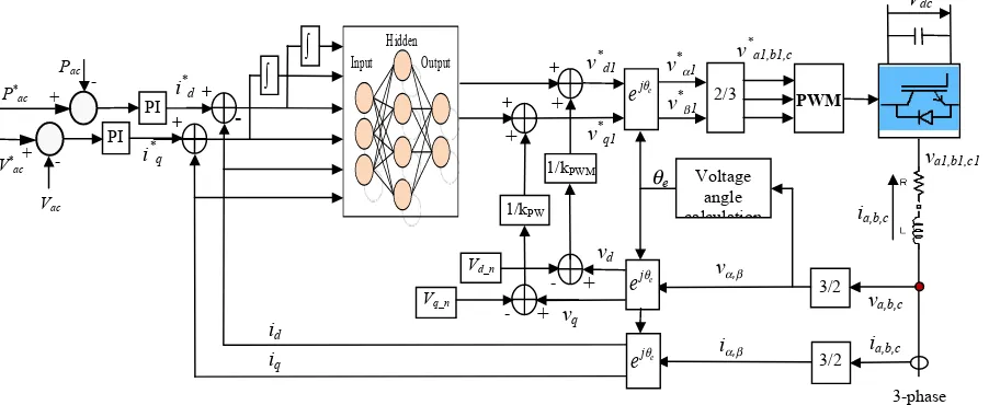
Following [6], and as in Fig. 1, our neural network vector control structure of a DER a d-axis loop is used for active power control and a q-axis loop is used for reactive power, or grid voltage support, control. The error signal between the measured and reference active power generates a d-axis current reference to the neural network through a PI controller, while the error signal between the actual and desired reactive power generates a q-axis current reference. The neural network, known here as the action network, is applied to the DER inverter through a pulse width modulation (PWM) mechanism to regulate the DER output voltage in the three-phase ac system. The ratio of the inverter output voltage to the output of the action network is a gain of kPWM, which equals Vdc/2 if the amplitude

The integrated DER system, described by Eq. (1), is rearranged into the standard state-space representation using Eq. (4), in which the system statesare idand iq, PCC voltages vdand vq normally are constant, and converter output

voltages vd1and vq1 are the control voltages to be specified by the output of the action network. For digital control

implementation and offline training of the neural network, the discrete equivalent of the continuous system state-space model, Eq. (4), must be obtained using Eq. (5), in which Ts represents the sampling period, k is an integer

time step, F is the system matrix, and G is the matrix associated with the control voltage. In this paper, a zero-order-hold discrete equivalent [8] is used to convert the continuous state-space model of the system in Eq. (4) to the discrete state-space model in Eq. (5). In all experiments, Ts=1ms.

d dt i_d i_q ⎡ ⎣ ⎢ ⎢ ⎤ ⎦ ⎥ ⎥=−

R_f L_f −ω_s ω_s R_f L_f

⎡ ⎣ ⎢ ⎢ ⎤ ⎦ ⎥ ⎥ i_d i_q ⎡ ⎣ ⎢ ⎢ ⎤ ⎦ ⎥ ⎥− 1 L_f

v_d1 v_q1

⎡ ⎣ ⎢ ⎢ ⎤ ⎦ ⎥ ⎥+ 1 L_f v_d v_q ⎡ ⎣ ⎢ ⎢ ⎤ ⎦ ⎥ ⎥ (4)

i_d

(

kT_s+T_s

)

i_q

(

kT_s+T_s

)

⎡ ⎣ ⎢ ⎢ ⎢ ⎤ ⎦ ⎥ ⎥ ⎥

=F id

( )

kTs

i_q

( )

kT_s

⎡ ⎣ ⎢ ⎢ ⎢ ⎤ ⎦ ⎥ ⎥ ⎥

+G vd1

( )

kTs −vd

v_q1

( )

kT_s −v_q ⎡ ⎣ ⎢ ⎢ ⎢ ⎤ ⎦ ⎥ ⎥ ⎥ (5)

The action network is a fully connected multi-layer perceptron [9] with six input nodes, two hidden layers having six nodes each, two output nodes, and shortcut connections between all pairs of layers, with hyperbolic tangent functions at all nodes. These six input components correspond to 1) the d- and q-axis current signals, 2) the two error signals of the d- and q-axis currents, and 3) the two integrals of the error signals. To simplify the expressions, the discrete system model in Eq. (5) is represented by:

!

i_dq

( )

k+1 =F⋅i!_dq

( )

k +G⋅

(

v!_dq1

( )

k -v!_dq

)

(6)

For a reference dq current,the control action applied to the system is expressed by:

PWM 3/2 3-phase supply 2/3 - +

v*a1,b1,c 1

vα,β

v* α1 v* β1 i* d Vdc va,b,c e j eθ - + i* q 3/2

iα,β ia,b,c

e j eθ id iq va1,b1,c1

∫

∫

Voltage angle calculation

Fig.1. Neural network vector control structure of DER converter. va1,b1,c1 represents the converter’s

output voltage in the three-phase ac system, and the corresponding voltages in the dq-reference frame are vd1 and vq1. va,b,c is the three-phase PCC voltage, and the corresponding voltages in the dq-reference

frame are vd and vq. ia,b,c represents the three-phase current flowing from the PCC to the converter, and

the corresponding currents in the dq-reference frame are id and iq. v*d1 and v*q1 are the d- and q-axis

voltages from the neural network controller, and the corresponding control voltage in the three-phase domain is v*

a1,b1,c1. ia,b,c θe + + + + v* d1 v* q1 +

[image:4.612.89.540.79.264.2]

!

v_dq1

( )

k =k_PWM⋅A

(

!i_dq

( )

k ,!i_dq

( )

k −!i_{dq_ref}

( )

k ,s!_dq(k),w!

)

(7)

in which

w

!

represents the weight vector of the action network, and

s

!

_dq

(

k

)

represents the network’s integral input vector defined by s(k)! =

(

!i_dq

( )

t −i!_{da_ref}

( )

t

)

dt

0

k

∫

.

3

NEURAL NETWORK TRAINING

Unlike the conventional standard vector controller, the neural network controller is produced through training using Dynamic Programming (DP). DP employs Bellman’s Principle of Optimality [10] and is a very useful tool for solving optimal control problems [11, 12]. The typical structure of discrete-time DP includes a discrete-time system model and a performance index or cost associated with the system [13]. The DP cost function associated with the vector-controlled system is defined as:

C i

(

!"!_dq

( )

j ,w"

)

= γk−j_U(e dq

! "!

(k))

k=j

∞

∑

,j>0,0<γ ≤1 (8)

in which γ is a discount factor, e! "_dq!(k)=

(

e_d(k),e_q(k)

)

=

(

i_d(k)−i_{d_ref}(k),i_q(k)−i_{q_ref}(k)

)

and U is defined as:

U(e! "!_dq(k))= e_d2_(k)+e q 2_(k)

⎡⎣ ⎤⎦α =

{

⎡⎣i_d(k)−i_{d_ref}(k)⎤⎦2+⎡⎣i_q(k)−i_{q_ref}(k)⎤⎦2

}

α

,α>0 (9)

in which

α

_{is a constant. The function} C(⋅), depending on the initial time jand the initial state i!"!_dq(j), is referred to as the cost-to-go of state i!"!_dq(j) of the DP problem. The objective of the neural network controller is to solve a current tracking problem, i.e., to hold the existing state i!_dq near a given (possibly moving) target state !i_dq*

so that the function C(⋅) _{in Eq. (11) is minimized. The current-loop action network was trained to minimize the}

DP cost in Eq. (11) using Levenberg-Marquardt backpropagation (LMBP) [9]. LMBP, a variation of Newton’s method, minimizes a function that is the sum of squares of a nonlinear function. Using LMBP with a general value for α requires a modification for the cost functionC( )⋅ defined in Eq. (8). Consider the cost function

C= γk−j_U(e

dq ! "!

(k))

k=j

∞

∑

, in which γ =1, j=1, and

k

=

1, , .

K

N

_Then, C can be written as:

C= U(e! "_dq!(k)) k=1

N

∑

=

( )

V(k) 2 k=1

N

∑

(10)

in which V(k)= U(e! "!_dq(k)) and the gradient ∂C/∂w!" can be written in matrix form as:

∂C ∂w!" =

∂

( )

V(k)2 k=1

N

∑

∂w!" = 2V(k) ∂V(k)

∂w!" k=1

N

∑

=2J(w!")T_V!"

in which V!"=⎡_⎣ V(1) … V(N) ⎤_⎦T, and the Jacobian matrix

J

(

w

!"

)

_is:

J(w!")=

∂V(1) ∂w1

! ∂V(1)

∂w_M

! " !

∂V(N)

∂w₁ !

∂V(N) ∂w_M ⎡

⎣ ⎢ ⎢ ⎢ ⎢ ⎢ ⎢ ⎢

⎤

⎦ ⎥ ⎥ ⎥ ⎥ ⎥ ⎥ ⎥

(12)

Therefore, the process of updating the weights using LMBP for a neural network controller can be expressed as:

Δw!"=−⎡J(w!")T_J(w!"_)+µI

⎣ ⎤⎦

−1

J(w!")T_V!" (13)

The parameterµwas dynamically adjusted to ensure that the training followed the decreasing direction of the cost function. When µincreased, (13) approached the steepest descent algorithm with a small learning rate, while as µ decreased, the algorithm (13) approached Gauss-Newton, which typically provides faster convergence. In order to increase the speed of computation, the weight update in Eq. (13) was conducted using Cholesky factorization, which is roughly twice as efficient as lower-upper decomposition for solving systems of linear equations [14].

To train the action network, the system data associated with Eq. (4) had to be specified. The training procedure for the current-loop action network involved: 1) randomly generating a sample initial state idq(j); 2) randomly

generating a changing sample reference dq current time sequence; 3) unrolling the trajectory of the system from the initial state; 4) training the current-loop neural network based on Eq. (13); and 5) repeating the process for all of the sample initial states and reference dq currents until reaching a stop criterion associated with the DP cost. All of the network weights initially were randomized using a uniform distribution with zero mean and 0.1 variance. The generation of the reference current considered the physical constraints of a practical DER inverter system. The randomly generated d- and q-axis reference currents first were chosen uniformly from [-Irated,Irated], in which Irated

represents the rated inverter line current. Then, these randomly generated d- and q-axis current values were checked and modified to ensure that their resultant magnitude did not exceed the inverter’s rated current limit and/or the control voltage did not exceed the converter’s PWM saturation limit. From the neural network standpoint, the PWM saturation constraint indicates the maximum positive or negative voltage that the action network can output. Therefore, if a reference dq current requires a control voltage that exceeds the acceptable voltage range of the action network, it is impossible to reduce the cost during the training of the action network.

The neural network controller is trained offline, and no training occurs in the real-time control stage. Without online training, a real-time control action can be computed very quickly using modern DSP chips. The most important issue is the sampling time. However, an optimal neural network controller can be trained using a large sampling time based on the DP principle, while tuning a conventional controller for the same sampling time could be very difficult or impossible. Therefore, the neural network controller actually has lesser sampling and computing power requirements during the real-time control process.

4

HARDWARE EXPERIMENT AND RESULTS

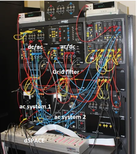
dSPACE digital control system [15]. The control system collects the dc-link voltage and three-phase currents and voltages at the PCC, and sends out control signals to the converter according to different control demands.

Fig. 2. Hardware laboratory testing and control systems

To ensure proper functioning of the neural network and conventional controllers, the test system was evaluated through computer simulation first before the hardware experiment. The simulation time step for the controllers was the same as the sampling time used in the dSPACE digital control system. Despite conducting simulation verification, the actual system performance in the hardware experiment environment could deteriorate due to unexpected disturbances, such as unbalanced grid-filter inductance, unbalanced and distorted grid voltage, and the deviation of system parameters from pre-measured values.

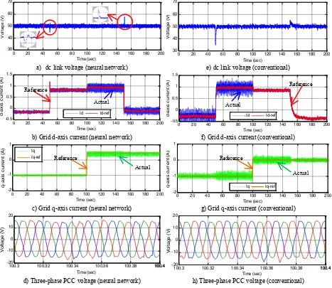
The test sequence was scheduled as follows, with t=0sec serving as the starting point for data recording. Around t=50sec, the active power transferred from the DER converter to the dc-link capacitor decreased. Around t=100sec, the value of the q-axis reference current changed from negative to positive, which corresponds to the reactive power reference changing from absorbing to generating. Around t=150sec, the active power transferred from the DER converter to the dc-link capacitor increased. The system data were not only collected by the dSPACE system, but also monitored by oscilloscopes and/or meters.

Fig. 3 shows the hardware experiment results. Compared to the standard vector control method, the neural network vector control approach demonstrated superior performance across various areas of functionality. When the dc-link voltage dropped due to a reduction of the active power transferred from the DER converter to the dc-link capacitor at approximately t=50sec, the controller quickly regulated the actual voltage to the reference value (Fig. 3a). As the reactive power demand changed from absorbing to generating around t=100sec, the actual q-axis current rapidly adjusted to the new q-axis current reference (Fig. 3c), and the oscillation of the dc-link voltage was very small. The converter was operating around the PWM saturation at this moment due to the generating reactive power; therefore, the q-axis current was unable to follow the reference current any better, causing the d- and q-axis currents to oscillate more because of the increased harmonic distortion. When the dc-link voltage increased due to a boost of active power transferred from the DER converter to the dc-link capacitor at approximately t=150sec, the controller quickly stabilized the dc-link capacitor voltage to the reference value (Fig. 3a). The neural network controller demonstrated great performance under all other conditions, even under the distorted PCC voltage in the laboratory condition (Fig. 3d).

[image:7.612.196.419.112.361.2]

the neural network based vector controller (Fig. 3a). In addition, the generation of the q-axis current reference for the conventional vector controller must assure that the converter operates well below the PWM saturation limit. Otherwise, the conventional vector control approach will go into a malfunction state. Other researchers also have reported the similar results, especially for converters in low-voltage applications [16-18].

a) dc link voltage (neural network) e) dc link voltage (conventional)

b) Grid d-axis current (neural network) f) Grid d-axis current (conventional)

c) Grid q-axis current (neural network) g) Grid q-axis current (conventional)

d) Three-phase PCC voltage (neural network) h) Three-phase PCC voltage (conventional)

Fig. 3. Hardware experiment evaluation using the conventional and neural network vector control mechanisms

Regarding the PCC voltage as shown in Figs. 3d and 3h, several factors contributed to the PCC voltage distortion. First, before conducting the experiment, we found that the three-phase voltage of the ac system was not perfectly sinusoidal. This voltage distortion resulted in more current harmonics during the vector control process. Second, the current harmonics generated by the power converter caused more PCC voltage distortion because of the equivalent ac system impedance. Third, the impact of the equivalent ac system impedance was significant in the low-voltage laboratory system.

5

CONCLUSIONS

This paper presented a neural network vector control mechanism for the control of a microgrid and the distributed energy sources within the microgrid. This controller, which implements dynamic programming, was trained with a

0 20 40 60 80 100 120 140 160 180 200 30 40 50 60 70 Time (sec) Vo lt a g e ( V)

0 20 40 60 80 100 120 140 160 180 200

30 40 50 60 70 Time (sec) Vo lta g e (V )

0 20 40 60 80 100 120 140 160 180 200

-0.5 0 0.5 1 1.5 Time (sec) d -a x is c u rre n t (A ) Id Id-ref

0 20 40 60 80 100 120 140 160 180 200

-0.5 0 0.5 1 1.5 Time (sec) d-ax is cu rren t (A ) Id Id-ref

0 20 40 60 80 100 120 140 160 180 200 -2 -1 0 1 Time (sec) q -a x is c u rre n t (A ) _Iq Iq-ref

0 20 40 60 80 100 120 140 160 180 200

-2 -1 0 1 Time (sec) q-ax is cu rren t (A ) Iq Iq-ref

100.3 100.32 100.34 100.36 100.38 100.4100.4

-20 -10 0 10 20 Time (sec) Vo lt a g e (V )

[image:8.612.74.541.134.539.2]

Levenberg-Marquardt backpropagation algorithm. Hardware experiments were conducted to evaluate the performance of the neural network vector control method. They showed that the neural network control technique performs well for DER converter control if the controller output voltage is below the converter’s PWM saturation limit. If the controller’s output voltage exceeds the PWM saturation limit, the neural network controller automatically turns into a state by maintaining a constant dc-link voltage as its first priority, while meeting the reactive power control demand as soon as possible. Under variable, unbalanced, and distorted system conditions, the neural network controller is stable and reliable.

REFERENCES

[1] A. Peças Lopes, C. L. Moreira, and A. G. Madureira, “Defining control strategies for microgrids islanded operation,” IEEE Trans. on Power Systems, vol. 21, no. 2, May 2006, pp. 916-924.

[2] B. Kroposki, R. Lasseter, T. Ise, S. Morozumi, S. Papatlianassiou, and N. Hatziargyriou, “Making microgrids work,” IEEE Power and Energy Magazine, vol. 6, issue 3, May-June 2008, pp. 40-53.

[3] F. Blaabjerg, R. Teodorescu, M. Liserre, and A. V. Timbus, “Overview of control and grid synchronization for distributed power generation systems,” IEEE Trans. Ind. Electron., 53: 5, pp. 1398–1409, 2006.

[4] P. Rodríguez, A. Luna, R. S. Muñoz-Aguilar, I. Etxeberria-Otadui, R. Teodorescu, and F. Blaabjerg, “A stationary reference frame grid synchronization system for three-phase grid-connected power converters under adverse grid conditions,” IEEE Trans. Power Electron., 27: 1, pp. 99–112, 2012.

[5] S. Li, M. Fairbank, C. Johnson, D. C. Wunsch and E. Alonso, “Artificial neural networks for control of a grid-connected rectifier/inverter under disturbance, dynamic and power converter switching conditions,” IEEE Trans. on Neural Net. and Learning Systems, 25: 4, pp. 738–750, 2014.

[6] S. Li, T.A. Haskew, Y. Hong, and L. Xu, “Direct-current vector control of three-phase grid-connected rectifier-inverter,”

Electric Power System Research (Elsevier), 81: 2, 2011, pp. 357-366.

[7] J. Rocabert, G. M. S. Azevedo, A. Luna, J. M. Guerrero, J. I. Candela, and P. Rodríguez, “Intelligent connection agent for three-phase grid-connected microgrids,” IEEE Trans. on Power Electronics, 26: 10, 2011, pp. 2993-3005.

[8] N. Mohan, T. M. Undeland, and W. P. Robbins, Power Electronics: Converters, Applications, and Design, 3rd ed., John Wiley & Sons Inc., 2002.

[9] G. F. Franklin, J. D. Powell, M. L. Workman, Digital Control of Dynamic Systems, 3rd ed., Addison-Wesley, 1998. [10]M. T. Hagan, H. B. Demuth, and M. H. Beale, “Neural Network Design,” Boston: PWS, 2002, ch. 12, pp. 19-23. [11]R. E. Bellman, Dynamic Programming. Princeton, NJ: Princeton Univ. Press, 1957.

[12]S. N. Balakrishnan and V. Biega, “Adaptive-critic-based neural networks for aircraft optimal control,” J. Guidance, Control, and Dynamics, 19: 4, pp. 893–898, 1996.

[13]H. He, N. Zhen, and F. Jian, “A three-network architecture for on-line learning and optimization based on adaptive dynamic programming,” Neurocomputing, 78: 1, pp. 3-13, 2012.

[14]F.Y. Wang, H. Zhang, and D. Liu, "Adaptive dynamic programming: An introduction," IEEE Comput. Intell. Mag., pp. 39–47, 2009.

[15]Embedded Success dSPACE DS1103 PPC Controller Board, available from:

tp://www.dspaceinc.com/en/inc/home/products/hw/singbord.cfm.

[16]M. Durrant, H. Werner, and K. Abbott, “Model of a VSC HVDC terminal attached to a weak ac system,” Proc.IEEE Conference on Control Applications, Istanbul, 2003.

[17]L. Zhang, “Modeling and control of VSC-HVDC links connected to weak ac systems,” Ph.D. dissertation, Royal Institute of Technology, Stockholm, Sweden, 2010.