Determining a new alignment scoring matrix for disordered proteins

(1)

Theses

Thesis/Dissertation Collections

2013

Determining a new alignment scoring matrix for

disordered proteins

Adam Handen

Follow this and additional works at:

http://scholarworks.rit.edu/theses

Part of the

Bioinformatics Commons

This Thesis is brought to you for free and open access by the Thesis/Dissertation Collections at RIT Scholar Works. It has been accepted for inclusion in Theses by an authorized administrator of RIT Scholar Works. For more information, please [email protected].

Recommended Citation

(2)

Determining a new alignment

scoring matrix for disordered

proteins

By

Adam Handen

A Thesis Submitted in Partial Fulfillment of the

Requirements for the Degree of Master of Bioinformatics

School of Life Sciences

College of Science

Rochester Institute of Technology

Rochester, NY

(3)

Committee:

Michael Osier, PhD

Gregory Babbitt, PhD

Gary Skuse, PhD

(4)

Abstract ... 3

Introduction ... 2

Materials and Methods ... 6

Results ... 16

Discussion ... 20

References ... 22

Table of Figures

Fig. 1. ATP Synthase ……….. 2

Fig. 2. Tp53 ……...……….. 4

Fig. 3. Structural Alignment of Tp53 ……….. 4

Fig. 4. Interactome of Tp53 ……...……….. 5

Fig. 5. GA Flowchart .……….. 7

Fig. 6. Sequence Alignment ...……….. 9

Fig. 7. Alignment Accuracy ………..………….. 11

Fig. 8. Beta Curve ...………..….. 13

Fig. 9. Matrix Recombination .……….... 14

Fig. 10. Matrix Mutation ...……….. 15

Fig. 11. Fitness Curve ...………17

Fig. 12. Generated Substitution Matrix ………... 18

Fig. 13. Non-Homologous Alignment Scores ..……….……….. 19

(5)

Abstract

Intrinsically disordered proteins (IDPs) are polypeptide sequences that do not form a rigid three

dimensional structure when isolated in the cytosol of the cell. These sequences are very common in most

genomes, and usually are involved in many protein-protein interactions. IDPs also play a key role in many

diseases, including cancer and Huntington’s disease. However, IDPs are difficult to study because of their

amorphous shape, high mutation rate, and unique amino acid composition. These obstacles make

homology studies especially difficult.

This study focused on generating a new substitution matrix designed to aid in homology studies

of IDPs. The matrix was generated using a genetic algorithm (GA). GAs are alternative hill-climbing

methods for finding solutions in complex problem spaces. To achieve this goal, a GA models the

evolutionary process found in nature by “breeding” solutions to the problem until one of sufficient quality

is produced.

The GA implemented in this study produced a substitution matrix for use in differentiation

between homologous and non-homologous proteins containing disordered regions. The matrix showed

some correlation to the patterns of evolution found in disordered proteins and their general sequence

makeup. However, when compared to a commonly used substitution matrix, BLOSUM, the GA’s

solution did not show significant improvement. But the results here do show a general proof of concept,

and that given modifications to the GA, more time, or more resources, a substitution matrix capable of

(6)

[image:6.612.189.397.240.507.2]

Fig. 1. 3D structure of ATP synthase from PDB [6]

a

b

Introduction

A proteins structure has traditionally been strongly associated with its function. One of the best

examples of this is ATP synthase. Each piece is able to function because of the shape it forms. The F0

subunit has pockets for protons to fit into, the axel is shaped to interlock with the F1 subunit, which in

turn opens and closes around ADP and inorganic phosphate (Figure 1) [1]. These rigid structures are what

allow ATP synthase to function, and this is true for most proteins as well.

The correlation between structure and function has led proteomics to focus on the rigid shape

polypeptides form. The Protein Data Bank, which stores 3D structures, has seen an exponential increase

in content, now numbering over 90,000 proteins [2]. Numerous computational methods have been

employed to try to predict the structures of proteins that have not been experimentally analyzed by X-ray

crystallography or NMR [3-5]. Some of these algorithms, such as I-TASSER, even make predictions of a

protein's function based on the assumed structure [3]. But what these methods cannot analyze, and what

(7)

Intrinsically disordered proteins (IDPs) are polypeptides that do not form a rigid structure when

isolated in the cytosol of the cell [7, 8]. The favored methods of studying the structure of proteins (x-ray

crystallography and NMR) do not provide much understanding of these polypeptides aside from

identifying them as disordered [9, 10, 11]. Because of this, many of the traditional methods for the study

of proteins cannot be applied to IDPs.

The amorphous shape of IDPs is because of their sequence. A high content of soluble amino acids

increases the sequences affinity to water, leading to the proteins flexibility [12, 13]. IDPs tend to have

very few hydrophobic amino acids, which usually form the interior of globular proteins, and also usually

lack bulkier amino acids [14]. This pattern was first observed in 1989 when it was found that unstructured

proteins also played a role in transcription regulation, making IDPs nothing new [15].

But despite having knowledge of IDPs for nearly 25 years, it is only recently that their

significance has been seriously analyzed. This is because of the historic concept that a protein requires a

rigid structure in order to function. Without a secondary or tertiary structure, IDPs have sometimes been

seen as filler for the proteome, assumed to be without use as non-coding DNA once was. The following

examples show the significance that IDPs may play in the proteome.

Knowing the general sequence signature of IDPs, many algorithms have been developed to

predict the proteome’s content of disordered regions. Predictive studies using these algorithms have

shown IDPs make up a significant portion of proteomes. One such study showed that two popular

prediction softwares, IUPred[16] and PONDR[17], both agreed that about 13% of E. coli’s proteome is

disordered, and nearly 60% of S. cerevisiae’s proteome[18]. Other estimates have suggested that up to

30% of proteins in eukaryotes could contain unstructured regions [19]. It would go against most

understanding of biology to assume that such a high proportion of the proteome would be without

function and still be retained.

Continued focus on IDPs has shown them to have significant functions within the cell. For

(8)

2). Homology studies have shown exactly how significant these disordered regions are to tp53’s function.

Overlaying the structures of tp53 and six of its homologues shows that the globular regions are nearly

identical (Figure 3). However, each of these proteins has very different functions. The homology study

concluded that the dramatic difference in the homologues functions was due to the differences in the

sequences at the N-terminus of each protein, an intrinsically disordered region [20]. Further studies on the

disordered region located at the N-terminus of tp53 have experimentally validated its significance,

showing that mutations in the sequence dramatically decrease tp53’s binding affinity to the other proteins

[image:8.612.92.254.275.470.2]

used for cell repair [21, 22].

Fig. 2. Structure of Tp53[23] Fig. 3. Structural alignment of Tp53 and seven of its homologues[20]

Another common feature between all of the tp53 homologues is their promiscuity. Tp53 is a

known hub in the human interactome, communicating with many other proteins to control the cell’s

activity when DNA damage is detected (Figure 4). This appears to be common among most IDPs, to be

highly interactive with other proteins [24]. This suggests that not only do IDPs have specific biological

(9)

[image:9.612.140.494.74.367.2]

Fig. 4. Interactome of Tp53 [25]

Given the high interactivity of IDPs, it comes as no surprise that they are also related to numerous

diseases. Mutations in tp53 are found in more than half of all cancers [26]. A myriad of other diseases,

such as Parkinson’s disease, mytonic dystrophy, Huntington’s disease, Machado-Joseph disease, and

numerous cancers are all related to mutations in disordered protein sequences [27, 28, 29]. The necessity

of functioning IDPs is at least as significant as that of globular proteins.

Though these conclusions have been drawn to show that IDPs are a necessity of cell life, there is

still very little known about them. This is mostly because the historical focus on a protein’s 3D structure

cannot be applied to IDPs. Furthermore, what is generally known about rigid proteins cannot be

transferred to IDPs. For example, the mutation rate of IDPs has been found to be significantly higher than

that of globular proteins, making homology studies difficult [30]. The specific amino acid mutation

frequencies also differ between these two classes of proteins, obviously because of their different needs

(10)

proteins, using the substitution matrices PAM and BLOSUM, are not nearly as effective on disordered

proteins [31].

The goal of this work was to create a method for generating a new substitution matrix that could

be used on disordered proteins to produce more accurate alignments and aid in homology studies among

disordered proteins.

Materials and Methods

To determine a new substitution matrix for disordered proteins, a genetic algorithm (GA) was

used. A GA is alternative to the general hill-climbing algorithm for finding a solution in a problem space.

The short coming of the hill-climbing algorithm is that it may easily be trapped in a local maximum,

never finding potentially higher quality solutions. GAs attempt to avoid this by modeling the evolutionary

process found in biology [32, 33].

Think on the finches studied by Charles Darwin. An initial population of birds migrated to an

island where the most abundant and nutritious food source was nuts. On the previous island, there had

been no evolutionary pressure for the birds to be able to eat nuts, and so the first generation on this new

island were a sort of random mixture of genotypes that may have had some ability to eat nuts, but most

had little or no ability to do so [34].

The finches that could manage to get some nutrition from the nuts would have been more fit.

Their higher fecundity would increase the number of birds in the next generation that would have some

ability to eat and digest nuts. With every generation, new genotypes would arise from recombination and

mutation, potentially producing birds with new or better ways to eat nuts. This continued until the

population reached a point where all birds could efficiently get nutrition from the nuts, and the

evolutionary pressure had been reduced by the genotype of the population.

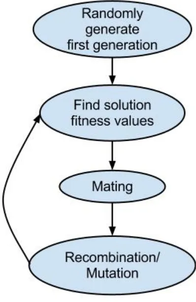
GAs attempt to model the same process that the finches went through. A set of solutions to a

given problem are generated as the initial population. The solutions are evaluated on their ability to solve

(11)

is then evaluated and bred. This process continues until a solution of sufficient quality is produced (Figure

[image:11.612.210.409.162.469.2]

5).

Fig. 5. Flow chart of a GA

Given the problem, finding a new substitution matrix for disordered proteins, the solutions used

for the GA in this project were substitution matrices. The initial population of matrices consisted of

twenty rows and columns, each representing a probability of mutation from one amino acid to another.

Matrix generation was done one column at a time. From left to right, each cell was assigned a random

value such that the column would sum to one. This was done by producing a random value greater than

zero and less than one minus the sum of the already assigned cells. There is an obvious bias here to the

(12)

column were shuffled after being generated. The population size for this GA was 25; each generation

consisted of 25 substitution matrices.

The solutions were also introduced to an environment. Where the finches had flown to a new

island covered with nut-bearing trees, the substitution matrices were given an environment of disordered

protein sequences. The initial set of sequences was retrieved from DisProt, a database dedicated to

collecting experimentally verified disordered sequences [35]. The sequences listed, however, were not all

complete. Some contained gaps, shown as an X in FASTA formatted files. For this study, sequences with

such gaps were removed. Each sequence was then run through BLAST to find homologous and

non-homologous sequences. Sequences that had an identity of 80-90% similarity were kept as non-homologous,

while sequences with an identity of 50-70% were kept as non-homologues. The BLAST results also had

to be screened for gaps, leaving 17,460 sequences. After discarding gapped BLAST sequences and any

DisProt sequences that had neither homologues nor non-homologues, 2,197 sequence clusters remained.

Each cluster began with a DisProt sequence, and contained a list of homologues and non-homologues for

the DisProt sequence. 70% of these clusters were used as the environment/training data for the GA, while

the remaining 30% were set aside for later evaluation.

The finches’ fitness was determined by its nutrition. In the GA, a solution’s fitness was

determined to be how well a substitution matrix could distinguish between homologues and

non-homologues. For this purpose, each substitution matrix had to align the DisProt sequence of each cluster

with all of the homologues and non-homologues for that cluster. The alignment process, however, was

incredibly time consuming. For a single substitution matrix to align all the sequences in the training data

using the Needleman-Wunsch method would take approximately 3 days. This was an unreasonable time

frame for the GA to run in. So an alternative method of alignment was implemented using sliding

windows.

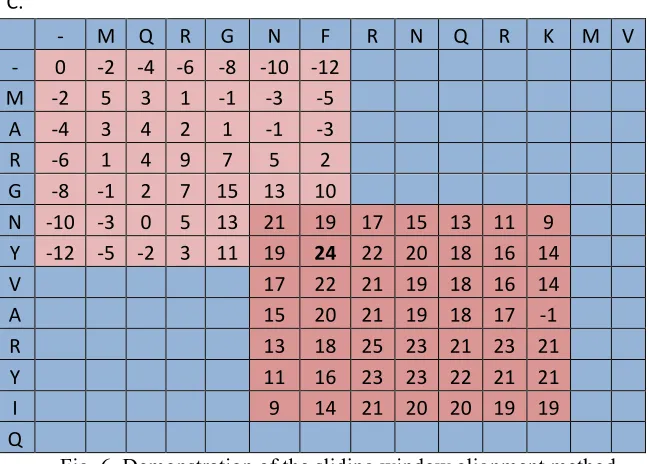
The sliding window method would take an initial portion of the alignment matrix from the

Needleman-Wunsch method. In this implementation, a seven by seven square was analyzed. The window

(13)

would define the location for the window to slide to. The window would move to put the highest value

the (1,1) position. The top-most row and left-most column would have any missing values filled in with

assumed gaps (Figure 6b), and then the Needleman-Wunsch method would be employed to fill in the rest

of the window (Figure 6c). This process would repeat until the bottom corner of the matrix was reached.

A.

-‐ M Q R G N F R N Q R K M V -‐ 0 -‐2 -‐4 -‐6 -‐8 -‐10 -‐12

M -‐2 5 3 1 -‐1 -‐3 -‐5

A -‐4 3 4 2 1 -‐1 -‐3

R -‐6 1 4 9 7 5 2

G -‐8 -‐1 2 7 15 13 10

N -‐10 -‐3 0 5 13 21 19

Y -‐12 -‐5 -‐2 3 11 19 24

V

A

R

Y

I

Q

B.

-‐ M Q R G N F R N Q R K M V -‐ 0 -‐2 -‐4 -‐6 -‐8 -‐10 -‐12

M -‐2 5 3 1 -‐1 -‐3 -‐5

A -‐4 3 4 2 1 -‐1 -‐3

R -‐6 1 4 9 7 5 2

G -‐8 -‐1 2 7 15 13 10

N -‐10 -‐3 0 5 13 21 19 17 15 13 11 9

Y -‐12 -‐5 -‐2 3 11 19 24

V

17 A

15 R

13 Y

11

I

9

Q

(14)

C.

-‐ M Q R G N F R N Q R K M V -‐ 0 -‐2 -‐4 -‐6 -‐8 -‐10 -‐12

M -‐2 5 3 1 -‐1 -‐3 -‐5

A -‐4 3 4 2 1 -‐1 -‐3

R -‐6 1 4 9 7 5 2

G -‐8 -‐1 2 7 15 13 10

N -‐10 -‐3 0 5 13 21 19 17 15 13 11 9

Y -‐12 -‐5 -‐2 3 11 19 24 22 20 18 16 14

V

17 22 21 19 18 16 14 A

15 20 21 19 18 17 -‐1 R

13 18 25 23 21 23 21 Y

11 16 23 23 22 21 21 I

9 14 21 20 20 19 19 Q

[image:14.612.146.471.78.310.2]

Fig. 6. Demonstration of the sliding window alignment method

The sliding window method greatly improves the run-time of the GA, reducing the time from 3

days to about 20 minutes per matrix. The speed gained by using the sliding window method increases

more for larger sequences, cutting out a large number of computations that would have otherwise been

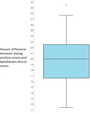
needed to find the global alignment. There is, however, a decrease in accuracy. Overall, the sliding

window method would produce alignment scores within about 20% of the actual score produced by using

the full Needleman-Wunsch alignment (Figure 7). This inaccuracy was considered to be acceptable for

(15)

Fig. 7. The quotient of the absolute value of the difference between the sliding window scores and Needleman-Wunsch scores.

The scores produced by the sliding-window alignment were used to determine a substitution

matrix’s fitness. However, the scores could not be used as they were. A sore from an alignment by the

Needleman-Wunsch algorithm, or by Smith-Waterman, is only comparable against other potential

alignments between those two same sequences. Otherwise, a 100% identity between two sequences of 30

amino acids may not be given as high a score as a 60% alignment between sequences of 200 amino acids.

To normalize the alignment scores for use in a fitness calculation, bit-scores were used instead.

Bit-scores are a normalized score used in BLAST searches to determine the likelihood of getting

the same quality alignment if a sequence was chosen at random. The bit-score calculation requires two

[image:15.612.171.466.75.447.2]

(16)

the dataset. They vary with the datasets size along with average sequence length. The only way to

determine the exact values to use is through an empirical analysis of the data, attempting to find the

probability that a sequence may have a higher score than a randomly selected one (Equation 2).

Fortunately, a pre-computed list of values based on different data sets was provided by the original

authors of bit-scores [36].

The fitness of a substitution matrix was defined as the sum of the bit-scores for the homologous

sequences minus the sum of the bit-scores of the non-homologous sequences. In this way, the most fit

substitution matrix should be able to better discriminate between homologous and non-homologous

among disordered proteins.

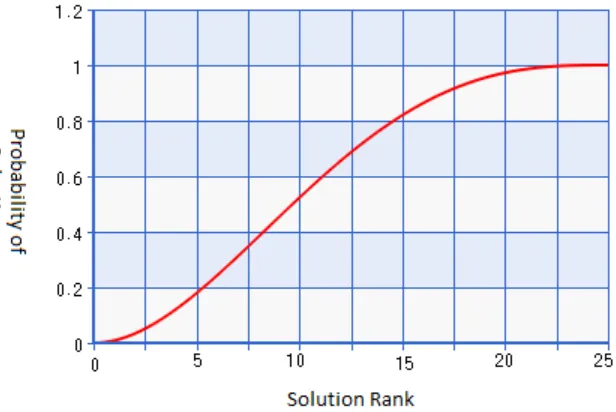
The fitness of a solution aids in its selection for breeding, just as the finches’ fitness did in the

Galapagos. Solutions were first sorted by their fitness, created a ranked list with 0 being the least fit and

24 being the most fit. The probability of selection was determined by using a beta-distribution (Figure 8).

This created a smooth slope that increased the chances of selecting a more fit solution for mating. What

this curve did not do was make it only possible for the most fit to mate. In order to keep heterogeneity in

the gene pool, less fit solutions were still given the opportunity to mate, just at a much lower frequency. Equation 1 – Bit-score calculation, where S is

the original alignment score

.

(17)

[image:17.612.110.418.77.283.2]

Fig. 8. Beta distribution for solution selection

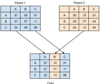
When two solutions were selected by the beta curve, a new substitution matrix was created by

recombination. The process is similar, though not identical to, recombination in our own biology, where

50% of the genetic material comes from one parents, and 50% comes from the other. For recombination

in the GA, the columns of the substitution matrices acted as chromosomes. For each column of the new

matrix, there was a 50/50 chance of using the choosing to copy the corresponding column from the first or

second parent (Figure 9). Given this, It was possible that all 20 columns could come from one parent and

no genetic material be contributed by the other. But probabilistically, 50% of the genetic material would

come from each parent matrix. The importance of this method is that the new matrix would still be viable.

That is, all of its columns would still sum to one. This removed the need to do additional checks on new

offspring and improved the GAs run time. The overall hope of using recombination is that good pieces of

(18)

[image:18.612.156.475.70.338.2]

Fig. 9. Demonstration of recombination in matrix mating

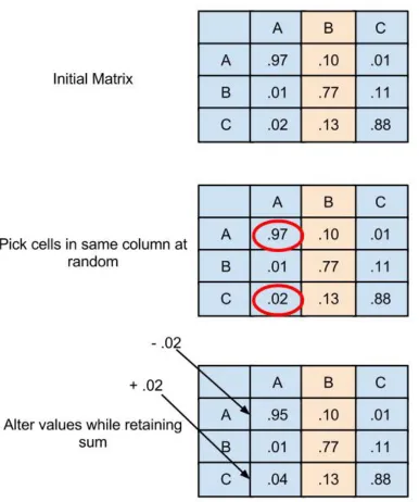
To add additional variation into the population, mutations were also performed on the new

matrix. Mutations in the finches are what allowed the short jumps forward to new genotypes that could

better eat nuts. Ideally, mutations in the GA would introduce new tricks into the substitution matrices that

could aid in differentiating between homologous and non-homologous IDPs. Mutations were performed

by selecting a column at random, and then two cells at random from within that column. A random

quantity from the first cell was then transferred to the second cell (Figure 10). The restrictions on the

amount moved between cells was that at the end, neither cell could be less than or equal to zero, or greater

(19)

[image:19.612.93.479.85.547.2]

Fig. 10. Demonstration of mutation within a matrix

A total of seven rounds of mutation were performed on each matrix generated through mating.

Because of the random selection process though, the number of altered cells was not a constant. The

amount transferred between cells could have been randomly selected to be zero, resulting in no effect.

There was also not check to see if the two cells selected for mutation were actually the same cell, which

(20)

well, effectively canceling out previous mutations. The result was that a matrix could have as many as 14

cells altered, but possibly less.

Each new generation consisted of 23 matrices produced by mating. The remaining two matrices

were taken from the previous generation. These two matrices were the best of that last generation.

Keeping a small proportion of the absolute best solutions helps keep track of the overall progress of the

GA, as well as prevents it from potentially going backwards from bad luck in mating.

In the real world, evolution never truly ends. There is still genetic fluctuation among the

Galapagos finches in their ability to eat nuts. But that variation is very low, mostly because the finches

have reached a point where their population is no longer under as much pressure to find a way to eat nuts

and so is not changing as rapidly. In the GA, there also comes a point where the population begins to

stagnate in its improvements, and the fitness of the best solution begins to form a plateau. This is when

the GA is terminated.

Results

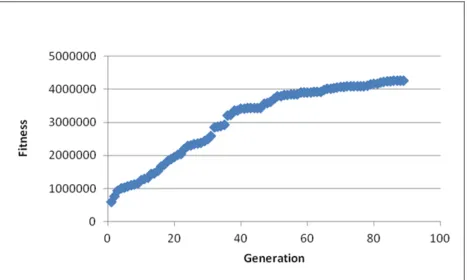
The GA was terminated after 10 days. In looking at the fitness of the best solution for each

generation, a plateau first appeared at day 5, near generation 50 (Figure 11). The GA was allowed to run

further though, and the maximum fitness continued to increase. When the GA had to be terminated due to

time restrictions, it was still unclear whether a plateau had really formed. It is possible that had the GA

(21)

[image:21.612.93.560.71.351.2]

Fig. 11. Graph of the fitness of the best solution for each generation of the GA

After terminating the GA, a substitution matrix was reported (Figure 12). The most immediately

visible trend in the matrix is that the mutation to lysine is highly favorable across the board. This is,

however, largely due to error. In the initial generation of matrices for the GA, there was an error in the

shuffling algorithm to remove the inherent bias in the random assignment of cell values. The shuffle

excluded the last column in its mixing, resulting in very high initial values. It is still likely that lysine

would be a favorable mutation, given its polarity and, therefore, affinity to water. But because of the error

in the shuffling algorithm, the results presented here cannot be used to interpret the significance of lysine

(22)

[image:22.612.72.545.96.435.2]

G A V L I S T C M P H R N Q E D F W Y K G 4 3 -3 0 1 2 2 0 -2 0 -13 4 1 1 2 2 0 1 -9 3 A 3 7 4 1 5 3 5 4 -10 4 3 -1 -7 -5 2 1 3 -14 -8 0 V -2 0 4 -6 3 -3 2 4 0 2 4 0 -8 1 -1 -1 -6 1 -2 2 L -12 3 0 4 2 -3 -1 -1 0 3 0 1 -2 -16 -5 -6 1 -11 2 0 I 4 3 1 5 4 0 -4 1 -2 -1 -4 0 -1 -1 2 2 -5 -6 2 5 S 3 2 1 3 -10 3 5 -5 -8 0 1 -6 -6 3 -10 0 -8 -9 4 3 T 3 5 4 2 1 3 6 3 2 3 1 4 -10 -13 0 -7 0 3 2 5 C -3 -11 5 -1 1 4 3 2 -2 1 0 2 0 0 -1 1 -12 -2 0 2 M 2 4 -2 -4 3 -3 0 -9 4 2 -9 -5 -1 3 4 -6 0 0 4 2 P 0 1 -1 2 4 2 3 -3 2 1 5 0 0 1 0 0 -5 -1 0 2 H 0 0 5 1 0 3 -2 3 3 -5 6 0 0 0 4 0 -10 0 6 1 R 1 -7 1 1 3 2 4 3 -3 2 5 4 -5 -1 -3 -7 -8 0 3 5 N -8 1 -1 -8 -20 2 2 -3 -21 -5 -1 2 5 -9 2 2 0 0 1 3 Q -4 -16 -13 3 4 2 5 -12 -5 1 0 4 -3 4 2 -2 1 -4 0 4 E 0 -6 -7 -9 -14 -12 6 -9 -10 0 1 0 2 3 4 1 2 -2 -6 3 D 0 5 2 1 3 -1 3 -18 0 0 4 1 -1 0 2 3 -11 2 -7 4 F 3 5 3 0 3 0 4 2 0 -1 -3 0 2 0 2 -10 4 -3 2 4 W 0 3 0 -1 -2 3 -1 -8 0 0 2 3 1 0 0 0 0 3 2 5 Y 2 -2 2 -8 0 6 -16 5 0 0 -11 6 -7 -3 2 -6 2 3 7 6 K -3 -6 5 3 -6 -10 6 -4 -4 -9 4 -2 0 0 2 -2 0 1 5 5

Fig. 12. Substitution matrix produced by the GA

Ignoring lysine, there were other amino acids that showed varying tendencies to mutate or be

conserved. Alanine and Tyrosine are the most conserved amino acids. Alanine is a common contributor to

alpha helices, and its hydrophobicity does tend to push this amino acid into the inside of the proteins

structure. Tyrosine is rather the opposite, being polar, bulky, and a common contributor to beta sheets. It

is interesting that these amino acids would be conserved more than those that do not have a tendency to

contribute to secondary structures. However, looking at the rate of conservation among the other amino

acids needed to form these secondary structures with alanine and tyrosine shows large variability. In fact,

the substitution matrix produced by the GA tends to favor mutation much more frequently than it does

(23)

conservation values range from 2 to 7, and has a median of only 4. Most of the amino acids even prefer

mutation, especially the hydrophobic amino acids. Nearly any mutation is favorable to tryptophan, and

the same goes for the other non-polars, with the exception of alanine and leucine.

Mutations to hydrophobic amino acids also appear highly unfavorable, getting scores as low as

-21. The lowest value on BLOSUM’s matrix is only -15. Non-polar amino acids are a major contributor to

folding as they try to stick to one another to avoid the polar solvent that is the cell’s body. To retain an

amorphous shape, it is only natural to expect IDPs to consist of mostly polar or charged amino acids.

Beyond comparing the composition of the GA’s result with BLOSUM, its effectiveness in

discerning between homologues and non-homologues had to be evaluated. The remaining test-data was

used for this analysis. Complete sequence alignments were used instead of the sliding-window method to

insure an accurate assessment of each matrix’s abilities at identifying similar sequences. When observing

the alignment of non-homologous sequences, the matrices should provide scores that are as low as

possible. When analyzing the differences in scores between BLOSUM and the GA’s matrix for this

analysis, the GA is competitive with BLOSUM. The median difference was only 2, meaning on average

[image:23.612.148.484.474.686.2]

the GA actually scored non-homologous sequences lower than BLOSUM (Figure 13).

(24)

The GA did not do as well on homologous sequences, however. Though there were instances in

which the GA did a better job identifying homologues, it scored most of the homologous pairs lower than

BLOSUM did. The median here was 93 when including the outliers, demonstrating that BLOSUM scored

homologous sequences much higher than the GA’s matrix (Figure 14). The difference is such that it

makes the GA’s edge in lowering the score of non-homologous pairs insignificant.

Fig. 14. The difference between BLOSUM’s scoring of homologous sequences and the scores of the GA.

Discussion

The substitution matrix produced by the genetic algorithm showed some correlation between

mutation frequency and the makeup of disordered proteins. There was a general preference for mutations

to small polar or charged amino acids, and a tendency to mutate from large and hydrophobic amino acids.

This pattern is what keeps disordered proteins fluid and flexible in the cytosol and prevents them from

forming the secondary and tertiary structures of globular proteins.

The score matrix also showed an overall favoritism to mutations, having very low numbers of

conservation of amino acids. The scores for conserving amino acids was two-thirds that of BLOSUM.

This matches the known trends for disordered proteins to mutate at a much higher frequency than

(25)

GA did not produce a matrix that could out-perform BLOSUM with sequence alignments. Though the

results between the GA’s alignments and BLOSUM’s were quite similar, BLOSUM consistently

differentiated between homologues and non-homologues better than the GA.

The factors that could have led to this result may have occurred as early as variable selection. Due

to the limited system resources, the GA’s population was kept incredibly small: only 25 solutions. In the

real world, a population this small would find it incredibly difficult to maintain genetic diversity. Using a

more reasonable population size of hundred, or even thousands of matrices would increase the diversity of

the gene-pool and increase the ability to sample the entire problem space. If there were either enough time

or more system resources, using a larger population would possibly produce a better solution after 100

generations.

The fitness curve also showed signs that the GA may not have reached a plateau in fitness values.

Even after almost 100 generations, it appears that more time could have been allowed to produce an even

better matrix. The time restraints on this project and the efficiency of the GA, however, required an early

termination. It is feasible that leaving the program to run for a longer period of time could have yielded a

matrix capable of discriminating between sequences better than BLOSUM.

Most of these issues were introduced because of a lack of resources and the time required for

sequence alignments. Using a massively parallel machine could allow the use of a larger population and

increase the number of generations analyzed in the same time frame. Another potential alteration would

be to change the dataset/environment. A smaller window for the homologous sequence score, say

85%-90% instead of 80-85%-90%, would reduce the number of sequence alignments that needed to be performed.

The same goes for the non-homologous sequence pairs. Decreasing the sequences selected to only

70-75% similarity would dramatically cut down the number of sequence comparisons needed to be

performed, and would therefore allow for more generations or a larger population.

Other potential improvements come at a coding level. The error that resulted in the bias toward

(26)

The constant favoritism to mutate to lysine in the final substitution matrix is strong evidence of the effect

of this particular mistake. Correcting this glitch in the code could not only produce a better substitution

matrix, but could also show better insight into the mutation patterns of disordered proteins.

The sliding-window method also decreased the accuracy of sequence alignments by an average of

20%. Using a full sequence alignment for the training data could have done a better job identifying which

substitution matrix really was the best at discriminating between homologues and non-homologous. If the

efficiency changes mentioned earlier were implemented, or if a machine as used capable of doing the full

alignments in less time, the use of the full Needleman-Wunsch algorithm could produce better results.

Though the GA did not manage to produce a substitution matrix that could out-perform

BLOSUM, it did come close. This indicates a fair proof of concept for the use of a GA to make a

substitution matrix for a specific class of proteins. Given more system resources and the afore-mentioned

improvements to the methodology, it is very likely that a genetic algorithm could yield a substitution

matrix that does a better job than BLOSUM for sequence alignments with disordered proteins.

References

1. Paul Boyer, “Toward an adequate scheme for the ATP synthase catalysis,”

Biochemistry(Moscow), 66(October 2001): 1058-1066.

2. David Goodsell, “ATP Synthase,” PDB Molecule of the Month (December 2005)

http://www.rcsb.org/pdb/101/motm.do?momID=72.

3. Yang Zhang, “I-TASSER server for protein 3D structure prediction,” BMC Bioinformatics,

9(2008): 40.

4. Yuedong Yang, Eshel Faraggi, Huiying Zhao, Yaoqi Zhou, “Improving protein fold recognition

and template-based modeling by employing probabilistic-based matching between predicted

one-dimensional structural properties of the query and corresponding native properties of templates,”

(27)

Journal of Molecular Biology, 339(June 2004): 591-605.

6. “Yearly Growth of Total Structures,” last modified July 16, 2013,

http://www.rcsb.org/pdb/statistics/contentGrowthChart.do?content=total&seqid=100.

7. Kieth Dunker, David Lawson, Celeste J. Brown, Ryan M. Williams, Pedro Romero, Jeong S. Oh,

Christopher J. Oldfield, Andrew M. Campen, Catherine M. Ratliff, Kerry W. Hipps, Juan Ausio,

Mark S. Nissen, Raymond Reeves, ChulHee Kang, Charles R. Kissinger, Robert W. Bailey,

Michael D. Griswold, Wah Chiu, Ethan C. Garner, Zoran Obradovic, “Intrinsically disordered

protein,” Journal of Molecular Graphics and Modelling, 19(February 2001): 26-59.

8. Peter E. Wright, Jane Dyson, “Intrinsically unstructured proteins: re-assessing the protein

structure-function paradigm,” Journal of Molecular Biology, 293(October 1999): 321-331.

9. Gary W. Daughdrill, Meggen S. Chadsey, Joyce E. Karlinsey, Kelly T. Hughes, Frederick W.

Dahlquist, “The C-terminal half of the anti-sigma factor, FlgM, becomes structured when bound

to its target, sigma28,” Nature Structural Biology, 4(1997): 285-291.

10. Jane Dyson, Peter E. Wright, “Unfolded Proteins and Protein Folding Studied by NMR,”

Chemistry Review, 104(2004): 3607-3622.

11. Oliver Hechta, Helen Ridleyb, Ruth Boetzela, Allison Lewina, Nick Culla, David A. Chaltonb,

Jeremy H. Lakeyb, Geoffrey R. Moore, “Self-recognition by an intrinsically disordered protein,”

FEBS Letters, 582(2008): 2673-2677.

12. Edward A. Weathersa, Michael E. Paulaitisa, Thomas B. Woolfb, Jan H. Hoh, “Reduced amino

acid alphabet is sufficient to accurately recognize intrinsically disordered protein,” FEBS Letters,

576(October 2004): 348–352.

13. Gerrit Praefckeab, Marijn Forda, Eva M. Schmid, Lene E. Olesen, Jennifer L. Gallop, Sew-Yeu

Peak-Chew, Yvonne Vallis, Madan Babu, Ian G. Millsc Harvey T. McMahon, “Evolving nature

of the AP2 alpha-appendage hub during clathrin-coated vesicle endocytosis,” The EMBO

(28)

14. Jane Dyson, Peter E. Wright, “Intrinsically Unstructured Proteins and Their Functions,” Nature

Reviews Molecular Cell Biology 6(March 2005): 197-208.

15. Pamela Mitchell, Robert Tjian, “Transcriptional regulation in mammalian cells by

sequence-specific DNA binding proteins,” Science, 245(July 1989): 371-378.

16. Zsuzsanna Dosztány, Veronika Csizmok, Peter Tompa, István Simon, “IUPred: web server for

the prediction of intrinsically unstructured regions of proteins based on estimated energy

content,” Bioinformatics 21(2005): 3433-3434.

17. Zoran Obradovic, Kang Peng, Slobodan Vucetic, Predrag Radivojac, A. Keith Dunker,

“Exploiting heterogeneous sequence properties improves prediction of protein disorder,” Proteins

61(2005): 176-182.

18. Peter Tompa, Zsuzsanna Dosztányi, István Simon, “Prevalent Structural Disorder in E. coli and S.

cerevisiae Proteomes,” J Proteome Res. 5(2006):1996-200.

19. Anthony L. Fink, “Natively unfolded proteins,” Current Opinion in Structural Biology,

15(February 2005): 35-41.

20. Bin Xue, Celeste J. Brown, A. Keith Dunker, Vladimir N. Uversky, “Intrinsically disordered

regions of p53 family are highly diversified in evolution,” Biochimica et biophysica acta. 4(April

2013): 725-38.

21. Daniel P. Teufel, Stefan M. Freund, Mark Bycroft, Alan R. Fersht, “Four domains of p300 each

bind tightly to a sequence spanning both transactivation subdomains of p53,” Proceedings of the

National Academy of Sciences of the United States of America, 104(April 2007): 7009-7014.

22. Mark Wells, Henning Tidow, Trevor J. Rutherford, Phineus Markwick, Malene Ringkjobing

Jensen, Efstratios Mylonas, Dmitri I. Svergun, Martin Blackledge, Alan R. Fersht, “Structure of

tumor suppressor p53 and its intrinsically disordered N-terminal transactivation domain,” ,”

Proceedings of the National Academy of Sciences of the United States of America, 105(April

(29)

http://www.rcsb.org/pdb/101/motm.do?momID=31.

24. Tanya Vavouri, Jennifer I. Semple, Rosa Garcia-Verdugo, Ben Lehner, “Intrinsic Protein

Disorder and Interaction Promiscuity Are Widely Associated with Dosage Sensitivity,” Cell,

138(July 2009): 198-208.

25. Amit U Sinha, Vivek Kaimal, Jing Chen, Anil G Jegga, “Dissecting microregulation of a master

regulatory network,” BMC Genomics 9(February 2008): 88.

26. “TP53,” Genetics Home Reference, last modified July 29, 2013,

http://ghr.nlm.nih.gov/gene/TP53.

27. Henry L. Paulson, Kenneth H. Fischbeck, “Trinucleotide Repeats in Neurogenetic Disorders,”

Annual Review of Neuroscience, 19(March 1996); 79-107.

28. Frederick C. Nucifora Jr., Masayuki Sasaki, Matthew F. Peters, Hui Huang, Jillian K. Cooper,

Mitsunori Yamada, Hitoshi Takahashi, Shoji Tsuji, Juan Troncoso, Valina L. Dawson5, Ted M.

Dawson, Christopher A. Ross, “Interference by Huntingtin and Atrophin-1 with CBP-Mediated

Transcription Leading to Cellular Toxicity,” Science 291(March 2001): 2423-2428.

29. Samuel Karlin, Luciano Brocchieri, Aviv Bergman, Jan Mrázek, Andrew J. Gentles, “Amino acid

runs in eukaryotic proteomes and disease associations,” Proceedings of the National Academy of

Sciences of the United States of America, 99(January 2002): 333-338.

30. Celeste J Brown, Audra K Johnson, Gary W Daughdrill, “Comparing Models of Evolution for

Ordered and Disordered Proteins,” Molecular Biology and Evolution 27(2010): 609-621.

31. Celeste J Brown, Audra K Johnson, A Keith Dunker, Gary W Daughdrill, “Evolution and

disorder,” Current opinion in structural biology 3(June 2011): 441-446.

32. Tom Mitchel, Machine Learning. New York: McGraw-Hill, 1997.

33. Melanie Mitchell, An Introduction to Genetic Algorithms. Cambridge: MIT, 1999.

(30)

35. Megan Sickmeier, Justin A. Hamilton, Tanguy LeGall, Vladimir Vacic, Marc S. Cortese, Agnes

Tantos, Beata Szabo, Peter Tompa, Jake Chen, Vladimir N. Uversky, Zoran Obradovic, A Keith

Dunker, “DisProt: the Database of Disordered Proteins,” Nucleic Acids Research, 35(January

2007): 786-793.

36. Stephen F. Altschul, Warren Gish, “Local Alignment Statistics,” Methods in Enzymology,