Transactions Letters
________________________________________________________________Adaptive Minimum Bit-Error Rate Beamforming
S. Chen, N. N. Ahmad, and L. Hanzo
Abstract—An adaptive beamforming technique is proposed based on directly minimizing the bit-error rate (BER). It is demonstrated that this minimum BER (MBER) approach utilizes the antenna array elements more intelligently than the standard minimum mean square error (MMSE) approach. Consequently, MBER beamforming is capable of providing significant perfor-mance gains in terms of a reduced BER over MMSE beamforming. A block-data adaptive implementation of the MBER beamforming solution is developed based on the Parzen window estimate of probability density function. Furthermore, a sample-by-sample adaptive implementation is considered, and a stochastic gradient algorithm, referred to as the least bit error rate, is derived. The proposed adaptive MBER beamforming technique provides an extension to the existing work for adaptive MBER equalization and multiuser detection.
Index Terms—Adaptive beamforming, bit-error rate (BER), mean square error, probability density function (pdf), smart antenna.
I. INTRODUCTION
T
HE ever-increasing demand for mobile communication capacity has motivated the employment of space-divi-sion multiple access for the sake of improving the achievable spectral efficiency. A particular approach that has shown real promise in achieving substantial capacity enhancements is the use of adaptive antenna arrays [1]–[10]. Adaptive beam-forming is capable of separating signals transmitted on the same carrier frequency, provided that they are separated in the spatial domain. A beamformer appropriately combines the signals received by the different elements of an antenna array to form a single output. Classically, this has been achieved by minimizing the mean square error (MSE) between the desired output and the actual array output. This principle has its roots in the traditional beamforming employed in sonar and radar sys-tems. Adaptive implementation of the minimum MSE (MMSE) beamforming solution can be realized using temporal reference techniques [2]–[4], [11]–[14]. Specifically, block-based beam-former weight adaptation can be achieved, for example, using the sample matrix inversion (SMI) algorithm [11], [12], while sample-by-sample adaptation can be carried out using the least mean square (LMS) algorithm [13], [14].For a communication system, it is the achievable bit-error rate (BER), not the MSE performance, that really matters.
Ide-Manuscript received April 27, 2002; revised May 7, 2003 and January 10, 2004; accepted January 16, 2004. The editor coordinating the review of this paper and approving it for publication is V. K. Bhargava.
The authors are with the School of Electronics and Computer Science, Uni-versity of Southampton, Southampton SO17 1BJ, U.K.
Digital Object Identifier 10.1109/TWC.2004.842981
ally, the system design should be based directly on minimizing the BER, rather than the MSE. For applications to single-user channel equalization and multiuser detection, it has been shown that the MMSE solution can in certain situations be distinctly inferior in comparison to the minimum BER (MBER) solution, and several adaptive implementations of the MBER solution have been studied in the literature [15]–[19]. This contribution derives a novel adaptive beamforming technique based on di-rectly minimizing the system’s BER rather than the MSE. For the sake of notational simplicity and for highlighting the basic concepts, the modulation scheme is assumed to be binary phase-shift keying (BPSK), and the channel is assumed to be nondis-persive with additive Gaussian noise, which does not induce any intersymbol interference (ISI). Furthermore, narrow-band beamforming is considered in this paper. It is demonstrated that the MBER solution utilizes the array weights more intelligently than the MMSE approach. The MBER beamforming appears to be “smarter” than the MMSE solution, since it directly op-timizes the system’s BER performance rather than minimizing the MSE, where the latter strategy often turns out to be deficient. An adaptive implementation of the MBER beamforming technique is investigated in this paper. The classic Parzen window or kernel density estimation technique [20]–[22] is adopted for approximating the probability density function (pdf) of the beamformer’s output, and a block-data adaptive MBER algorithm is developed, which iteratively minimizes the estimated BER of the beamformer by adjusting the beamformer weights using a simplified conjugate gradient optimization method [23], [19]. Our simulation study shows that this block-data adaptive MBER algorithm converges rapidly, and the length of the data block required for achieving an accurate approximation of the MBER solution is reasonably small. Sample-by-sample adaptation is also considered and an adap-tive stochastic gradient MBER algorithm, referred to as the least BER (LBER) technique, is derived. This LBER algorithm involves more approximations compared with the one given in [18] and [19] for equalization and multiuser detection, but it has a significantly lower computational complexity, which is comparable to that of the simple least mean square (LMS) algorithm. Simulation results suggest that the proposed simplified LBER algorithm has a similar performance to the full-complexity LBER algorithm of [18], [19] in terms of its convergence rate and steady-state BER misadjustment.
II. SYSTEMMODEL
It is assumed that the system supports users (signal sources), and each user transmits a BPSK modulated signal on
the same carrier frequency of . Let denote the bit instance. Then, the baseband signal of user is formulated as
(1)
where takes value from the set with equal proba-bility and denotes the signal power of user . Without loss of generality, source 1 is assumed to be the desired user and the rest of the sources are the interfering users. The linear antenna array considered consists of uniformly spaced elements, and the signals received by the -element antenna array are given by
(2)
where is the relative time delay at array element for source is the direction of arrival for source , and is the complex-valued white Gaussian noise having a zero mean and a variance of . The desired user’s signal-to-noise ratio (SNR) is defined as , and the desired signal-to-interference ratio (SIR) with respect to user is defined
as , for . In vectorial form, the
array input can be expressed
as
(3)
where has a covariance
ma-trix of with representing the
identity matrix, the system matrix is given by
(4)
the steering vector for source is formulated as
(5)
and the transmitted bit vector is .
The beamformer’s output is given by
(6)
where is the complex-valued beamformer
weight vector, and is Gaussian distributed having a zero
mean and a variance of . The
esti-mate of the transmitted bit is given by
(7)
where denotes the real part of .
Classically, the beamformer’s weight vector is determined by
minimizing the MSE term of , which leads to the following MMSE solution:
(8)
with being the first column of . Although the system matrix is generally unknown, the MMSE solution can be readily re-alized using the block-data based adaptive SMI algorithm [11], [12]. The MMSE solution can also be implemented using the stochastic gradient algorithm known also as the LMS algorithm. The discrete Fourier transform (DFT) of the beamformer weights, which is also referred to as the beam pattern, is given by
(9)
which describes the response of the beamformer to the source arriving at angle . In traditional beamforming, the magnitude of is used for characterizing the performance of a beam-former. Using the amplitude response alone, however, can be misleading, since both the magnitude and phase of should be used together for characterizing the beamformer. Ultimately, it is the pdf of the beamformer’s output which fully character-izes the true performance of the beamformer.
III. MBER BEAMFORMINGSOLUTION
Denote the number of possible transmitted bit se-quences of as . Further, denote the first element of , corresponding to the desired user, as . The array input signal takes values from the signal set defined as
(10)
This set can be partitioned into two subsets depending on the specific value of as follows:
(11)
Similarly, the beamformer’s output takes values from
the scalar set . Thus,
the real part of the beamformer’s output can only take values from the set
(12)
which can be divided into two subsets conditioned on as follows:
(13)
such that the two scalar sets and are com-pletely separable by a linear decision boundary. Otherwise, linear beamforming is required, a situation that is similar to non-linear single-user equalization and nonnon-linear multiuser detec-tion [24]–[26].
It can be readily shown that the conditional pdf of
given is
(14)
where and is the number of
the points in . Thus, it can be shown that the BER of the beamformer associated with the weight vector is given by
(15)
where
(16)
and
(17)
Similarly, the BER can be calculated using . The MBER beamforming solution is then defined as
(18)
The gradient of (15) with respect to can be shown to be
(19)
Given the gradient of (19), the optimization problem (18) can be solved by iteratively using a gradient-based optimization algo-rithm. Since the BER is invariant to a positive scaling of , it is computationally advantageous to normalize to a unit length after every iteration so that the gradient can be simplified to
(20)
The following simplified conjugate gradient algorithm [23], [19] provides an efficient means of finding a MBER solution.
Initialization: Choose a step size of and a termination scalar of (typically, can be set to the machine accuracy);
given and , set the iteration index
to .
Loop: If
: gotoStop. Else
for , gotoLoop.
Stop: is the solution.
The step size controls the rate of convergence. Typically, a much larger value of can be used compared to the steepest descent gradient algorithm. Occasionally, the search direction in the above conjugate gradient algorithm may no longer be a good approximation to the conjugate gradient direction or may even point to the “uphill” direction when the iteration index be-comes high. A standard measure to prevent this situation from happening is to periodically reset to the negative gradient [23]. With a reseting of every iteration, this algorithm reduces to the steepest descent gradient algorithm.
Unlike the MMSE solution (8), there exists no closed-form MBER solution. In theory, there is no guarantee that the above conjugate gradient algorithm can always find a global minimum point of the BER surface . In practice, we have found that the algorithm works well and we have never observed any occurrence of the algorithm being trapped at some local min-imum solution. This is likely to be a consequence of the specific shape of the BER surface. Since the BER is invariant to a pos-itive scaling of , i.e., the size of does not matter (except zero size), the BER surface has an infinitely long valley, and any point at the bottom of this valley is a true global MBER so-lution. For an illustration, see [19]. Once a weight vector is near the edge of this infinitely long valley, convergence to the bottom is extremely fast since the slope or gradient is high.
IV. ADAPTIVEMBER BEAMFORMING
The pdf of can be shown to be explicitly given by
(21)
and the BER can alternatively be expressed as
where
(23)
and . In reality, the pdf of is
un-known. Hence, we will adopt the temporal reference technique for supporting the adaptive implementation of the MBER beam-forming algorithm.
A. Block-Data-Based Gradient Adaptive MBER Algorithm
A widely used approach of approximating a pdf is known as the kernel density or Parzen window-based estimate [20]–[22]. Given a block of training samples , a kernel density estimate of the pdf (21) is readily given by
(24)
where the kernel width is related to the standard deviation of the channel noise. From the standard results [20]–[22], it is known that the Parzen window estimate (24) is not overly sensitive to the value of , and appropriate values for lie in a range of values between some lower and upper bounds. From this estimated pdf, the estimated BER is given by
(25)
with
(26)
The gradient of is formulated as
(27)
Upon substituting by in the conjugate gra-dient updating mechanism, a block-data based adaptive algo-rithm is obtained. The step size and the kernel width are two algorithmic parameters that have to be set appropriately.
B. Stochastic Gradient-Based Adaptive MBER Algorithm
In the kernel density estimate (24), a variable width of is used, which depends on the beamformer’s weight vector. If an approximation is invoked by using a constant width of in a kernel density estimate, the associated computational complexity can be considerably reduced. Formally, this leads to using the kernel density estimate of
(28)
TABLE I
COMPARISON OFCOMPUTATIONALCOMPLEXITYPERWEIGHTUPDATE, WHERE
LIS THEDIMENSION OF THEWEIGHTVECTOR
as an approximation to the true density given by (21) and to using
(29)
with
(30)
as the BER estimate. This approximation is valid, provided that the width is chosen appropriately. In particular, the appro-priate values for in (28) are generally different from those used in (24). Like the kernel density estimate (24), the pdf estimate (28) is not overly sensitive to the value of . The gradient of
has a much simpler form
(31)
In order to derive a sample-by-sample adaptive algorithm, adopt a similar single-sample estimate of as used in [18], namely
(32)
Using the instantaneous stochastic gradient of
(33)
gives rise to a stochastic gradient adaptive algorithm, which we referred to as the LBER algorithm
(34)
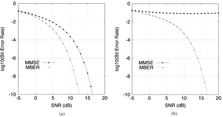
Fig. 1. Comparison of the BER performance of the MMSE and MBER beamformers: (a)SIR = 0dB fori = 2; 3; 4; 5and (b)SIR = 06dB fori = 2; 3; 4; 5.
involves a more coarse approximation and exhibits a lower com-putational complexity.
V. SIMULATIONSTUDY
The example used in our computer simulation study consisted of five signal sources and a two-element antenna array. The an-tenna array element spacing was with being the wave-length. The direction of arrival for source 1, the desired user, was 15 , and the directions of arrival for the interfering sources 2, 3, 4, 5 were 30 , 60 70 , and 80 , respectively. Fig. 1 com-pares the BER performance of the MBER solution with that of the MMSE solution under two different conditions: (a) the de-sired user and all the four interfering sources have equal power and (b) all the four interfering sources have 6-dB higher power than the desired user. The BER curves in Fig. 1 were computed using the theoretical BER expression (15) with the MMSE so-lution given by (8) and the MBER soso-lution obtained by numer-ical optimization based on the simplified conjugate gradient al-gorithm portrayed in Section III. For this example, the supe-rior performance of the MBER beamforming technique over the MMSE benchmarker scheme becomes evident. The results shown in Fig. 1 also indicate that the MBER solution is robust to the near–far effect. This is further confirmed by the result shown in Fig. 2, which was obtained under the following
con-dition: dB and dB for were
fixed, while was varied.
Fig. 3 compares the beam pattern of the MBER beamformer to that of the MMSE beamformer under the condition of
dB and dB for , where has
been normalized. Note that the MMSE beamformer appears to have a better amplitude response than the MBER beamformer. Specifically, at the four angles corresponding to the four inter-fering sources indicated by the circles in Fig. 3, the MMSE beamformer exhibits higher attenuation magnitude responses at 70 , 60 , and 80 , and only a slightly inferior magnitude re-sponse at 30 , compared to the MBER solution. If the ampli-tude response alone would constitute the ultimate performance criterion of a beamformer, the MMSE beamformer would ap-pear to be more beneficial. However, considering the
magni-Fig. 2. Influence of near–far effect on BER performance of the MMSE and MBER beamformers forSNR = 10dB andSIR = 24dB fori = 3; 4; 5.
tude response alone can be misleading. At the four angles of the four interfering sources, the phase response of the MBER beam-former is significantly closer to than that of the MMSE solution while maintaining a 0 phase for the desired user at the angle of 15 . Thus, the MBER solution has a significantly better response in terms of , and this results in an augmented ability to “cancel” interfering signals. Explicitly, the two beam-formers optimize the beamformer weights very differently.
It is seen that the operation of the MMSE beamformer ap-pears to break down under the conditions given in Fig. 1(b) and exhibits a high BER floor. A first attempt of interpreting this phenomenon is made by examining the beam patterns of the
two beamformers given dB and dB for
[image:5.594.339.511.291.468.2]perfor-Fig. 3. Comparison of MMSE and MBER beam patterns forSNR = 10dB andSIR = 0dB fori = 2; 3; 4; 5.
mance. The conditional pdfs of the two beamformers, under the
conditions of maintaining dB and dB
for , are illustrated in Fig. 4. In Fig. 4, the beam-former’s weight vector has been normalized to a unit length so that the BER is mainly determined by the minimum dis-tance of the subset from the decision threshold of . There are points altogether due to five users, calculated based on the formula where is the number of users. By examining Fig. 4, it becomes clear why the MMSE beamformer has a high BER floor of around (1.5/16). For the MMSE solution, and
are linearly nonseparable. One of the
points in is on the wrong side of the decision boundary of and another point is right on . By comparison, it can be seen from Fig. 4 that the MBER solution
successfully separates and .
Let us now study the performance of the block-data-based gradient adaptive MBER algorithm employing the conjugate gradient updating mechanism. Fig. 5 illustrates the convergence rate of the algorithm under the conditions of dB,
dB, dB, and a block
size of , using two different initial weight vectors,
namely: (a) and (b)
[image:6.594.48.281.59.341.2]. From Fig. 5, it can be seen that this block-data-based adaptive algorithm converges rapidly. The effect of the block size on the performance of the block-data-based adaptive MBER algorithm was also investigated, and it is seen that in conjunction with a short block length of , the BER per-formance of the block-data-based adaptive MBER solution de-grades only slightly at high SNRs compared to the theoretical
Fig. 4. Conditional pdfs givenb (k) = +1and subsetsY (w)of the MMSE and MBER beamformers forSNR = 15dB andSIR = 06dB for
i = 2; 3; 4; 5: (a) MMSE and (b) MBER.
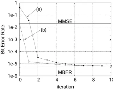
Fig. 5. Convergence rate of the block-data-based gradient adaptive MBER algorithm of Section IV-A for a block size ofK = 200under the conditions
SNR = 10dB,SIR = SIR = 06dB, andSIR = SIR = 0dB. (a)w(0) = [0:1 + j0:00:1 + j0:0] ; = 0:8and = 2 = 0:1. (b)
w(0) = w ; = 0:5and = 2 = 0:1.
MBER solution. When the block length increases to , the block-data based adaptive MBER solution closely matches the performance of the theoretical MBER solution. Space con-straints preclude a graphical illustration. The performance of the stochastic gradient-based adaptive MBER algorithm por-trayed in Section IV-B is investigated next. Fig. 6 shows the learning curves of the LBER algorithm using two different ini-tial weight vectors under the conditions of dB,
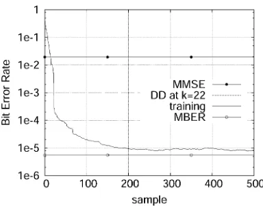
[image:6.594.316.544.64.370.2] [image:6.594.332.520.430.578.2]Fig. 6. Learning curves of the stochastic gradient adaptive MBER algorithm of Section IV-B averaged over 20 runs. SNR = 10 dB,
SIR = SIR = 06dB, and SIR = SIR = 0 dB. DD denotes decision-directed adaptation in which b (k) is substituted by its estimate
^b (k). Note that in graph (b) decision-directed and training curves are indistinguishable. (a)w(0) = [0:1 + j0:00:1 + j0:0] ; = 0:03 and
= 4 = 0:2. (b)w(0) = w ; = 0:02and = 4 = 0:2.
be seen that this stochastic gradient algorithm converges rea-sonably fast while maintaining a low steady-state BER misad-justment.
To explicitly investigate the influence of weight initializa-tion on the LBER algorithm, 20 uniformly distributed random initial weight were used, under the conditions of
dB, dB, and
[image:7.594.330.522.63.213.2]dB. Fig. 7 depicts the learning curves obtained. Note that a vari-able adaptive step size was used, where over each randomly ini-tialized run for the first 25 samples we had , which was reduced to afterward. The need for an adaptive step size may be explained as follows. When is far from the MBER solution, the gradient of the BER surface can be very flat and hence a large adaptive step size is needed to move away from these flat regions. By contrast, as mentioned at the end of Sec-tion III, once is near the edge of the “infinitely long MBER valley,” convergence to the bottom is extremely fast and a small step-size is required to avoid “over-shooting” the MBER solu-tion. It is also worth pointing out that the MMSE solution is not necessarily a “favorable” initial condition for the LBER algo-rithm. For the example simulated here, the algorithm appeared to converge well when started from , as can be
Fig. 7. Learning curves of the stochastic gradient adaptive MBER algorithm of Section IV-B averaged over 20 randomly chosen uniformly distributed initial weight valuesw(0).SNR = 10dB,SIR = SIR = 06dB, andSIR =
SIR = 0dB. DD denotes decision-directed adaptation in whichb (k)is substituted by its estimate^b (k). Note that the performance curves based on DD and explicit training are indistinguishable. Furthermore, we had = 4 =
0:2and = 0:2for the first 25 samples, reducing the step size to = 0:02 afterwards.
seen from Fig. 6(b). However, as confirmed in many other in-vestigations not included here due to lack of space, the MMSE solution often constitutes an undesirable initial condition, which results in slow convergence and a relatively high steady-state BER misadjustment. To provide a rule of thumb, if the interfer-ence scenario encountered is a hostile one due to having a low angular separation of the interferers, for example, the MMSE weights would be far from the MBER solution and hence they would result in slow convergence, potentially arriving at a local optimum.
VI. CONCLUSION
An adaptive MBER beamforming technique has been devel-oped. It has been shown that the MBER beamformer exploits the system’s resources more intelligently than the standard MMSE beamformer and, consequently, can achieve a better performance in terms of a lower BER. Simulation results also suggest that the MBER solution is robust to the near–far effect. Adaptive implementation of the MBER beamformer has also been addressed. A block-data-based conjugate gradient adaptive MBER algorithm has been shown to converge rapidly while requiring a reasonably small block size for accurately approximating the theoretical MBER solution. A stochastic gradient adaptive MBER algorithm, namely the LBER tech-nique, has also been derived. The results obtained in this study have demonstrated the potential of the adaptive MBER beamforming approach. However, several important areas still warrant further research. These include considering hostile fading channels, dispersive wideband channels that induce ISI, and wideband beamforming. Our current research is also considering the extension of the adaptive MBER beamformer to other modulation schemes.
REFERENCES
[image:7.594.63.261.63.393.2][2] M. C. Wells, “Increasing the capacity of GSM cellular radio using adap-tive antennas,”IEE Proc. Commun., vol. 143, no. 5, pp. 304–310, 1996. [3] J. Litva and T. K. Y. Lo,Digital Beamforming in Wireless
Communica-tions. London, U.K.: Artech, 1996.
[4] L. C. Godara, “Applications of antenna arrays to mobile communica-tions, Part I: Performance improvement, feasibility, and system consid-erations,”Proc. IEEE, vol. 85, no. 7, pp. 1031–1060, Jul. 1997. [5] A. J. Paulraj and C. B. Papadias, “Space-time processing for wireless
communications,”IEEE Signal Process. Mag., vol. 14, no. 6, pp. 49–83, 1997.
[6] J. H. Winters, “Smart antennas for wireless systems,” IEEE Pers. Commun., vol. 5, no. 1, pp. 23–27, Jan. 1998.
[7] R. Kohno, “Spatial and temporal communication theory using adaptive antenna array,”IEEE Pers. Commun., vol. 5, no. 1, pp. 28–35, 1998. [8] P. Petrus, R. B. Ertel, and J. H. Reed, “Capacity enhancement using
adap-tive arrays in an AMPS system,”IEEE Trans. Veh. Technol., vol. 47, no. 3, pp. 717–727, 1998.
[9] G. V. Tsoulos, “Smart antennas for mobile communication systems: Benefits and challenges,”IEE Electron. Commun. J., vol. 11, no. 2, pp. 84–94, 1999.
[10] J. S. Blogh and L. Hanzo, Third Generation Systems and Intelli-gent Wireless Networking—Smart Antennas and Adaptive Modula-tion. New York: Wiley, 2002.
[11] I. S. Reed, J. D. Mallett, and L. E. Brennan, “Rapid convergence rate in adaptive arrays,”IEEE Trans. Aerosp. Electron. Syst., vol. AES-10, pp. 853–863, 1974.
[12] M. W. Ganz, R. L. Moses, and S. L. Wilson, “Convergence of the SMI and the diagonally loaded SMI algorithms with weak interference (adaptive array),”IEEE Trans. Antennas Propagat., vol. 38, no. 3, pp. 394–399, Mar. 1990.
[13] B. Widrow, P. E. Mantey, L. J. Griffiths, and B. B. Goode, “Adaptive antenna systems,”Proc. IEEE, vol. 55, pp. 2143–2159, 1967. [14] L. J. Griffiths, “A simple adaptive algorithm for real-time processing in
antenna arrays,”Proc. IEEE, vol. 57, pp. 1696–1704, 1969.
[15] S. Chen, B. Mulgrew, E. S. Chng, and G. Gibson, “Space translation properties and the minimum-BER linear-combiner DFE,”IEE Proc. Commun., vol. 145, no. 5, pp. 316–322, 1998.
[16] I. N. Psaromiligkos, S. N. Batalama, and D. A. Pados, “On adaptive min-imum probability of error linear filter receivers for DS-CDMA chan-nels,”IEEE Trans. Commun., vol. 47, no. 7, pp. 1092–1102, Jul. 1999. [17] C. C. Yeh and J. R. Barry, “Adaptive minimum bit-error rate
equaliza-tion for binary signaling,”IEEE Trans. Commun., vol. 48, no. 7, pp. 1226–1235, Jul. 2000.
[18] B. Mulgrew and S. Chen, “Adaptive minimum-BER decision feedback equalisers for binary signalling,”Signal Process., vol. 81, no. 7, pp. 1479–1489, 2001.
[19] S. Chen, A. K. Samingan, B. Mulgrew, and L. Hanzo, “Adaptive minimum-BER linear multiuser detection for DS-CDMA signals in multipath channels,”IEEE Trans. Signal Process., vol. 49, no. 6, pp. 1240–1247, Jun. 2001.
[20] E. Parzen, “On estimation of a probability density function and mode,”
Ann. Math. Stat., vol. 33, pp. 1066–1076, 1962.
[21] B. W. Silverman,Density Estimation. London, U.K.: Chapman Hall, 1996.
[22] A. W. Bowman and A. Azzalini,Applied Smoothing Techniques for Data Analysis, Oxford, U.K.: Oxford Univ. Press, 1997.
[23] M. S. Bazaraa, H. D. Sherali, and C. M. Shetty,Nonlinear Programming: Theory and Algorithms. New York: Wiley, 1993.
[24] S. Chen, B. Mulgrew, and P. M. Grant, “A clustering technique for dig-ital communications channel equalization using radial basis function networks,”IEEE Trans. Neural Networks, vol. 4, no. 4, pp. 570–579, Aug. 1993.
[25] S. Chen, B. Mulgrew, and S. McLaughlin, “Adaptive Bayesian equaliser with decision feedback,”IEEE Trans. Signal Process., vol. 41, no. 9, pp. 2918–2927, Sep. 1993.
[26] S. Chen, A. K. Samingan, and L. Hanzo, “Support vector machine multiuser receiver for DS-CDMA signals in multipath channels,”IEEE Trans. Neural Networks, vol. 12, no. 3, pp. 604–611, Jun. 2001. [27] S. Chen, “Least bit error rate adaptive multiuser detection,” in Soft