Numerical study of PPE source term errors in the incompressible SPH models

This is a repository copy of Numerical study of PPE source term errors in the incompressible SPH models.

White Rose Research Online URL for this paper: http://eprints.whiterose.ac.uk/86321/

Version: Accepted Version

Article:

Gui, Q., Dong, P. and Shao, S. (2014) Numerical study of PPE source term errors in the incompressible SPH models. International Journal for Numerical Methods in Fluids, 77 (6). 358 - 379. ISSN 0271-2091

https://doi.org/10.1002/fld.3985

[email protected] https://eprints.whiterose.ac.uk/ Reuse

Unless indicated otherwise, fulltext items are protected by copyright with all rights reserved. The copyright exception in section 29 of the Copyright, Designs and Patents Act 1988 allows the making of a single copy solely for the purpose of non-commercial research or private study within the limits of fair dealing. The publisher or other rights-holder may allow further reproduction and re-use of this version - refer to the White Rose Research Online record for this item. Where records identify the publisher as the copyright holder, users can verify any specific terms of use on the publisher’s website.

Takedown

If you consider content in White Rose Research Online to be in breach of UK law, please notify us by

1

Numerical Study of PPE Source Term Errors in the

Incompressible SPH Models

Qinqin Gui1, Ping Dong2 and Songdong Shao3

1 PhD candidate, Department of Civil Engineering, University of Dundee, Dundee, DD1 4HN, United Kingdom. Email: [email protected]

2 Professor, Department of Civil Engineering, University of Dundee, Dundee, DD1 4HN, United Kingdom. Email: [email protected]

3 Senior Lecturer, Department of Civil and Structural Engineering, University of Sheffield, Mappin Street, Sheffield, S1 3JD, United Kingdom (Kunlun Scholar Professor, College of Hydraulic and Hydroelectric Engineering, Qinghai University, Xining 810016, China ; Visiting Professor, State Key Laboratory of Hydro-Science and Engineering, Tsinghua University, Beijing 100084, China ). Email: [email protected]

Abstract

In a recent work by Gui et al. (2014) [Gui, Q., Shao, S. and Dong, P. (2014), Wave impact simulations by an improved ISPH model, Journal of Waterway, Port, Coastal and Ocean Engineering, ASCE, 140(3), 04014005], an incompressible SPH model was presented that employs a mixed pressure Poisson equation (PPE) source term combining both the density-invariant and velocity divergence-free formulations. The present work intends to apply the model to a wider range of fluid impact situations in order to quantify the numerical errors associated with different formulations of the PPE source term in ISPH models. The good agreement achieved between the model predictions and documented data is taken as a further demonstration that the mixed source term formulation can accurately predict the fluid impact pressures and forces, both in the magnitude and in the spatial and temporal patterns. Furthermore, an in-depth numerical analysis using either the pure density-invariant or velocity divergence-free formulation has revealed that the pure density-invariant formulation can lead to relatively large divergence errors while the velocity divergence-free formulation may cause relatively large density errors. As compared with these two approaches the mixed source term formulation performs much better having the minimum total errors in all test cases. Although some recent studies found that the weakly compressible SPH (WCSPH) models perform somewhat better than the incompressible SPH models in certain fluid impact problems, we have shown that this could be largely caused by the particular formulation of PPE source term in the previous ISPH models and a better formulation of the source term can significantly improve the accuracy of ISPH models.

Keywords: ISPH, PPE, source term error, mixed source term, density-invariant, velocity

2

Introduction

The study of fluid impact on structures is of significant importance to understand the underlying physics of the hydrodynamic phenomena as well as to evaluate the structure stability so as to take effective measures to prevent possible structure damage and functional failure. Although laboratory experiments and field measurements were traditionally used to study such a problem, numerical simulations have also increasingly been used as an attractive alternative technique, being free from the scale effect associated with the physical models and much cheaper than the field measurements.

In recent years, the mesh-free particle models have become popular to investigate different fluid impact problems, as these kinds of models can naturally describe the large deformation of free surfaces and material interfaces and thus avoid the complicated mesh readjustment, which is unavoidable in the mesh-based approaches. This advantage arises from the fact that in a mesh-free particle method the advection term in the hydrodynamic equations is calculated directly by each individual particle and thus the numerical diffusions can be reduced to minimum. Currently two particle modelling techniques are frequently reported in the hydraulic and coastal hydrodynamic computations, i.e. the Moving Particle Semi-implicit (MPS) (Khayyer and Gotoh, 2009) and Smoothed Particle Hydrodynamics (SPH) (Gomez-Gesteira et al., 2005) methods.

The SPH method originated in the astronomic applications (Lucy, 1977) and its potentials in the fluid flow computations were developed by Monaghan (1992). In the early fluid impact simulations by SPH, the fluid media were treated as slightly compressible so the method was regarded as the WCSPH (Monaghan et al., 2003). However, as the computation of fluid pressure was based on an equation of state which was in nature related to the thermodynamic formulation, relatively large pressure fluctuations and noises were inevitable, and this could greatly compromise the simulation accuracy. Following the novel SPH projection approach (Cummins and Rudman, 1999), different incompressible SPH (ISPH) models were widely developed in recent years. The key feature of this approach is that the fluid pressure is solved by using a truly hydrodynamic formulation based on the pressure Poisson equation (PPE) in a similar manner to most mesh-based hydrodynamic schemes. Quite a few works have demonstrated that the ISPH model could predict a more stable pressure and particle fields than the WCSPH in fluid impact situations and also no additional numerical smoothing techniques, such as the XSPH or kernel corrections are needed.

3

both of which were rooted in the projection concept of Cummins and Rudman (1999) but they were applied in the free surface flows. However, extensive applications of ISPH for the fluid impact problems have disclosed that the density-invariant and velocity divergence-free approaches could not provide identical impact pressures and forces, although both schemes were consistent in satisfying the incompressible principle. For example, Xu et al. (2009) found that the divergence-free ISPH method could not maintain the stability in certain situations although it was fairly accurate before the instability set in, while the density-invariant ISPH method was stable but often associated with the random-noise like disturbance. On the other hand, Cummins and Rudman (1999) and Hu and Adam (2007) found that if only a discrete velocity divergence-free condition was enforced, larger density-variation or particle clustering may occur due to the spatial truncation errors of the discretization scheme and the density errors could accumulate during long time computation. To make full use of the advantage of both projection schemes, Asai et al. (2012) and Gui et al. (2014) combined both the density-invariant and divergence-free terms in a simple and straightforward PPE source term representation and they found that the wave impact predictions on the collapse of a water column were much improved. Similar combination technique was also adopted in other particle-based methods like the Consistent Particle Method (CPM) (Koh et al., 2013).

Recently a number of studies have been carried out to address pros and cons of the WCSPH and ISPH for the free surface flow simulations. Hughes and Graham (2010) studied two standard dam-break problems and found that the WCSPH performed at least as well as the ISPH, and in some respects clearly performed better. Shadloo et al. (2012) studied the bluff body flow problem such as the flow over an airfoil and square obstacle, and their predictions of a variety of flow parameters indicated that the WCSPH method with suggested implementations produced the numerical results as accurate and reliable as those of the ISPH. Chen et al. (2013) investigated three benchmark hydrodynamic problems including a liquid sloshing and they concluded that their improved WCSPH was much more attractive than the ISPH in modelling the free surface incompressible flows, as the former was more accurate and stable but also with comparable or even less computational effort. It should be noted that the above-mentioned WCSPHs have included some additional numerical treatments to improve the model performance, such as the MLS/Shepard density filter (Gomez-Gesteira et al., 2010) or XSPH, while there was no such treatment in the ISPHs so the comparisons of two techniques were not made on an equal basis.

4

works on the study of density accumulation errors in the ISPH projection scheme based on the velocity divergence-free approach (Cummins and Rudman, 1999; Szewc et al., 2012), but there is almost no detailed study reported for the divergence errors in a density-invariant ISPH approach. The pressure noises and particle fluctuations in a density-invariant ISPH could be attributed to quite a few complicated mechanisms but the velocity divergence error could be just one important factor that caused the inaccuracy. In this work we will show that with the decrease of divergence error the pressure noises and prediction errors can also be reduced accordingly.

The structure of this paper is as follows: In the next section, a review of two standard ISPH projection schemes and the combined mixed source term formulation by Gui et al. (2014) are presented. Then the treatment of free surface and boundary conditions is briefly described to close the model. In the model applications and validations, three benchmark fluid impact problems including two dam break flows and one solitary wave impact are computed by using three different ISPH numerical schemes, respectively, and the computational results are validated against either the experimental or numerical data based on the MPS/WCSPH. Finally, an in-depth numerical analysis is carried out to quantify the density and divergence errors of three different ISPH numerical schemes.

ISPH Model with Three Different Projection Schemes

Governing Equations

The governing equations to simulate the vertical 2D flows are the mass and momentum conservation equations. With regard to the fluid particle in an ISPH scheme, the Lagrangian form of the Navier-Stokes (N-S) equations is used:

0 1

  

 u

dt d

 Eq. (1)

u g

u 2

0

1 _{   }



 

 P

dt d

Eq. (2)

where  = fluid particle density; t = time; u = particle velocity; P = pressure; ₀ = kinematic viscosity; and g = gravitational acceleration.

ISPH Solution Procedure

5

projection scheme of Chorin (1968). Cummins and Rudman (1999) first introduced the ISPH projection method to enforce the incompressibility in a correction step. The prediction step in the ISPH is usually an explicit integration in time using the viscous and gravitational forces. So an intermediate particle velocity and position is calculated from the momentum equation (2) as:

u_* (g₀2u)_tt Eq. (3)

*

* u u

u  t Eq. (4)

r*rtu*t Eq. (5)

where u_* = changed particle velocity during the prediction step; t = time increment; u t

and r = particle velocity and position at time t t ; and u* and r* = intermediate particle

velocity and position.

Then, in the final correction step, the pressure term is incorporated into the momentum Eq. (2) to update the intermediate particle velocity and position as below:

t P_t

t    



 



1 * 1

* *

1



u u

u Eq. (6)

* * *

1 u u

ut_   Eq. (7)

t

t t t

t 

 

 



2 )

( ₁

1

u u r

r Eq. (8)

where _* = intermediate particle density after the prediction step; P = particle pressure; _t1 and ut1 and r = particle velocity and position at time t1 t1.

Recently many other forms of ISPH solution procedures have been used to improve the numerical performance. For example, the gravitational force in momentum equation (2) was included in the correction step by Liu et al. (2013) to improve the hydrostatic simulation. In Chen et al. (2013), a half-time scheme that included two loops within one time step involving

t and t1 values was used and the numerical scheme could achieve second-order accuracy.

Different PPE Source Term Formulations

6





 u** Eq. (9)

where 0 = initial constant particle density. By combining Eqs. (6) and (9), Shao and Lo

(2003) first proposed the ISPH Pressure Poisson equation (PPE) based on the relative density variance as follows:

0 1 2 0 1 t P t       _  _ 

  Eq. (10)

Alternatively, by projecting the intermediate particle velocity field onto a divergence-free space, the divergence of Eq. (6) can be written as:

1 1 1 t t P

t _ 

     _{ } _  _      + * u u Eq. (11)

As for a truly incompressible scheme, the fluid density should be constant and thus Eq. (1) is reduced to the following formulation in discrete form

1 0

t

u₊  Eq. (12)

By considering a constant density field and combining Eqs. (9), (11) and (12), the following PPE with the velocity divergence source term is obtained (Hu and Adam, 2007; Lee et al., 2008): 1 1     _  _ 

 Pt  t

*

u

Eq. (13)

Here it should be noted that the projection schemes to enforce the fluid incompressibility in Eqs. (10) and (13) are exactly equivalent in the theory, but numerically some researchers have found their performances could be different (Asai et al., 2012; Gui et al., 2014). Generally it has been agreed that the density-invariant formulation Eq. (10) can well conserve the fluid volume and thus is numerically quite stable, but it could generate relatively large pressure noises and particle fluctuations (Xu et al., 2009). This is due to that the SPH summation scheme of fluid density is very sensitive to the particle position and a small error in the particle locations could generate a large density disturbance. On the other hand, the velocity divergence-free formulation Eq. (13) is much less sensitive to the error of particle positions so it can give very smooth pressure field. However, as the fluid volume is not exactly conserved especially after a long time simulation, the model can become unstable due to the compression of the fluid and particle penetration of the solid boundaries.

7

approaches through a simple weighting coefficient, has been developed in the Consistent Particle Method (CPM) by Koh et al. (2013). Similar works have also been done by Asai et al. (2012) and Gui et al. (2014). This hybrid PPE source term is generally represented as:

t t

P_t

       

 

 _ *

2 0

* 0

1) (1 )

1

(  u

   

 Eq. (14)

However, quantifying the value of weighting coefficient  in different applications is not an easy task. By trading off between the pressure fluctuation and fluid volume conservation, Koh et al. (2013) recommended a value of 0.5 for their benchmark sloshing problem. In Asai et al. (2012), they found that the coefficient was not a constant but largely dependent on the particle spacing. In Gui et al. (2014), they used the energy dissipation principle and related the weighting coefficient with representative height-depth ratio of the flow system. An even more advanced weighting coefficient has been developed by Khayyer and Gotoh (2011) based on the dynamic instantaneous flow field. It is clear that more works are still required in evaluating the weighting coefficient in this type of mixed source term. In the present study, as our focus is on evaluating the density and divergence errors of three different projection schemes in Eqs. (10), (13) and (14), no further attempt will be made on the choice of weighting coefficient .

Basic SPH Formulations

The key feature of the SPH is that it is an interpolation method which allows any function and physical value to be expressed in terms of its value at a set of disordered points. In numerical simulations the integral interpolant is calculated by a summation interpolant in the discrete notation as:

 



 

a b ab

b b

A

A r m r W Eq. (15)

where A r

 





ab a b

W W r r ,h = kernel weight function, in which h = smoothing length. The kernel function is the fundamental in the SPH scheme. In this work we use the kernel based on the spline function in Monaghan (1992). Only particles within twice of the smoothing length contribute to the values of a reference particle.

8

a b ab

b m W





 Eq. (16)

The gradient of pressure at a given particle can be written in many different ways, such as the following one used in this paper

2 2

1 a b

b a ab

b a b

a

P P

P m   W

 _  _{  }

 

 

 



where _aW_ab is the gradient of the kernel taken with respect to the position of particle a. The divergence of vector u at a given particle can be computed by:

a b a b a b b a

a  m   W



 ) 1



( u u u

 Eq. (18)

Due to the high sensitivity to the pressure noise and particle disorder, the Laplacian in PPE Eqs. (10), (13) and (14) is formulated by using a hybrid of the standard SPH first derivative combined with a finite difference scheme as (Shao and Lo, 2003)





1 8 _{ab ab a ab}

b b

a a b ab

P W P m    _  _     



    Eq. (19)

where P_ab P_aP_b and r_ab  r_a r are defined; and _b  is a small number to maintain non-singularity and commonly set at 0 1. h in the SPH practice. Similarly the viscous term in momentum Eq. (2) can also be formulated by following the derivation of above Laplacian as

2 2 2 0 ) ( 2 ) (             



b a b

b a b a W m r r u

u Eq. (20)

where ua b ua ub is defined.

Free Surfaces and Solid Boundaries

9

Recently Khayyer et al. (2009) and Liu et al. (2013) introduced a complementary free surface criterion based on the particle symmetry, but this criterion must be used together with either the density or the divergence criterion. Otherwise the free surface particles could be identified incorrectly. In this work, we simply apply the density criterion to judge the free surface without further investigation.

Generally, there are three common wall boundary treatments widely reported in the SPH literatures, i.e. the repulsive boundary in the original WCSPH (Monaghan, 1992), mirror particle boundary in Cummins and Rudman (1999) and fixed dummy particle boundary in Shao and Lo (2003). The first one is the most straightforward to implement but can generate unrealistic flow patterns near the wall region, while the second one could be the most accurate in dealing with both the non-slip and slip solid boundaries but at the sacrifice of computational effort. Here we adopt the last dummy particle method because this can give satisfactory result at reasonable CPU resources. It needs to be pointed out that the dummy particles used in the present work are similar to the dynamic boundary particles used by Crespo et al. (2007) but they differ in that the former uses the co-located particle arrangement and also the dummy particles are not involved in the integration of any equations, while the latter boundaries are constituted by the particles initially placed in a staggered grid manner and they then move following the same equations of state and continuity as the inner fluid particles.

In the density-invariant ISPH scheme, two lines of the dummy particles are used in order to keep the fluid density at wall particles consistent with the inner fluids. On the other hand, in the divergence-free ISPH scheme, by following Monaghan and Kajtar (2009) a reduction of the boundary particle spacing is used to prevent particle penetration through the solid boundaries. Besides, four layers of the dummy particles are used because more neighbouring particles are needed for the calculation of velocity divergence in the pressure Poisson equation. In both projection schemes, the velocities of the wall and dummy particles are set zero to represent the non-slip boundary condition. The wall particles are also involved in the PPE solution during which the homogeneous Neumann boundary condition is imposed.

Model Applications and Validations

10

Dam Break Flow Simulations

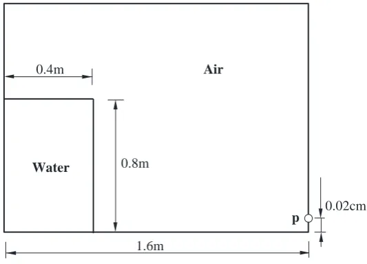
The numerical simulation is carried out in a 2D tank as shown in Fig. 1. The dimension of the numerical tank is 1.6 m by 1.6 m in square. The initial static water column of 0.4 m wide and 0.8 m high is retained by an instantaneously removed vertical wall. Then the water flows along the horizontal bed and hits the right wall generating a high impact pressure. To validate the accuracy of ISPH pressure computations, a reference point (P) located on the right wall at a distance of 0.02 m from the bottom is used to record the ISPH data. The ISPH computed pressures will be compared with the improved MPS results by Lee et al. (2011) who used a step by step improvement in their numerical algorithm.

Fig. 1 Schematic sketch of dam break problem in Lee et al. (2011)

In the ISPH simulation, to be consistent with Lee et al. (2011) the initial particle spacing was selected as X = 0.01 m and thus 3200 fluid particles in total were used. The simulation was carried out up to 3 s. Here it should be noted that in a series of numerical MPS improvements adopted by Lee et al. (2011), a mixed PPE source term that is similar to Eq. (14) was also used and they recommended the weighting coefficient in the equation to be 0.01 ~ 0.05. In the ISPH model, the determination of weighting coefficient  in Eq. (14) was made on the energy dissipation mechanism that is related to the height-depth ratio of the flow H/L (Gui et al., 2014). By using this principle,  was evaluated to be around 0.03, which falls nicely within the value range of 0.01 ~ 0.05 in Lee et al. (2011).

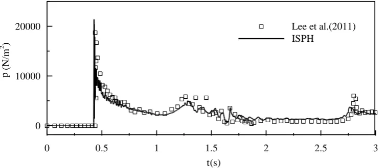
Fig. 2 shows the comparison of pressure computations at measuring point P made by the ISPH with mixed source term Eq. (14) and the improved MPS proposed by Lee et al. (2011). It demonstrates a quite satisfactory agreement between the two numerical time histories of the wave impact pressure. Both results reported almost identical peak wave arrival time at three different time instants: the first largest one that happened before time t = 0.5 s, which

0.4m

0.8m

0.02cm

p Water

1.6m

11

was due to the dam break wave hitting the right side wall and thus generating a quite large pressure impact; the second one that happened around t = 1.3 s, which was due to the falling water plunging down towards the water surface; and the third one that happened about t = 2.8 s, which was due to the reflected return dam break wave impacting on the right wall again but this time at a much smaller amplitude. The ISPH computations match the first two peak values well but underpredict the third one. In the step-by-step improvement of the MPS algorithms in Lee et al. (2011), quite a few numerical treatments were used including the optimisation of collision coefficient, revision of the source term and gradient model, improvement of the surface particle search, etc. while in the present ISPH model only the mixed source term formulation is adopted but it can still give equally good prediction. Here it should be clarified that the computed pressure at measuring point P was obtained by interpolating the pressures of wall particles adjacent to point P on the right wall.

Fig. 2 Time histories of computed pressures by ISPH and improved MPS model of Lee et al. (2011)

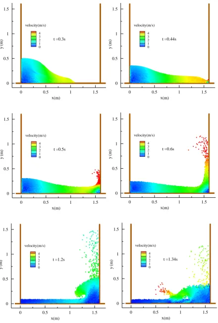
To demonstrate the general dam break flow features, the computed ISPH particle snapshots with the velocity contours are shown in Fig. 3 at several typical times. The computations showed the dam break flows impacted on the right wall at time t = 0.44 s and ran along against the wall to reach maximum height at t = 0.6 s. Then the flows plunged down on the water surface and created a second splash at t = 1.34 s. The velocity contours indicated that larger flow velocities always appeared near the flow front and smaller flow velocities were found upstream of the original dam site. Also, by comparing with the particle snapshots computed by Lee et al. (2011) using the original and improved MPS, it can be seen that the present ISPH simulations are much better than the original MPS results in view of reducing the particle fluctuation. However, the ISPH simulated particle snapshots still contain more noises than the improved MPS results, as the latter used several complementary numerical schemes to improve the model performance.

t

p

0 0.5 1 1.5 2 2.5 3

0 10000

20000 Lee et al.(2011)

ISPH

(s)

(N

/m

12

Fig. 3 ISPH computed particle snapshots with velocity contours at different times x

y

0 0.5 1 1.5

0 0.5 1 1.5 4 3 2 1 0 =0.3s velocity(m/s) t (m) (m ) x y

0 0.5 1 1.5

0 0.5 1 1.5 4 3 2 1 0 =0.44s velocity(m/s) t (m) (m ) x y

0 0.5 1 1.5

0 0.5 1 1.5 4 3 2 1 0 =0.5s velocity(m/s) t (m) (m ) x y

0 0.5 1 1.5

0 0.5 1 1.5 4 3 2 1 0 =0.6s velocity(m/s) t (m) (m ) x y

0 0.5 1 1.5

0 0.5 1 1.5 4 3 2 1 0 =1.2s velocity(m/s) t (m) (m ) x y

0 0.5 1 1.5

13

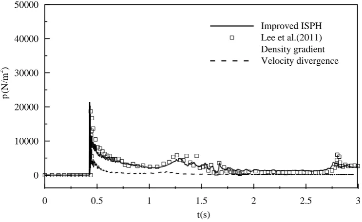
To further demonstrate the difference of using different PPE source term formulations, additional two ISPH runs were made, in which only the density-invariant or velocity divergence-free scheme as given by Eq. (10) or (13) was used, and the simulation results of time history of wave impact pressures are compared with the mixed source term results based on Eq. (14) and the improved MPS computations of Lee et al. (2011) in Fig. 4. It showed that the pure density-invariant ISPH model predicted a consistently higher pressure evolution and also relatively larger pressure fluctuations. Although the general pressure time histories followed the correct trend, the pressure amplitude at some time instants can be overestimated by up to several times due to the existence of pressure noise. On the other hand, the pure velocity divergence-free ISPH model predicted a much smaller and smoother pressure process without any pressure fluctuations observed. However, it can barely capture the first pressure peak and fail completely in predicting the second and third pressure peaks due to numerical damping caused by the compression of the fluid volume. The pressure amplitudes were significantly underestimated as a result. In comparison, the mixed source term ISPH model provided the most promising result.

Fig. 4 Time histories of computed pressures (at measuring point P) by three different ISPH source terms and compared with improved MPS results of Lee et al. (2011)

Solitary Wave Propagation and Impact

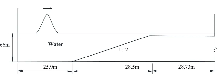
In this section, the proposed ISPH model is used to reproduce a physical experiment (Robertson et al., 2013) involving a solitary wave propagating and shoaling over a 1:12 beach slope and a flat reef, then turning into a turbulent bore and colliding with a solid wall which is located 83 m away from the offshore wave maker. According to Robertson et al. (2013),

t

p

0 0.5 1 1.5 2 2.5 3

0 10000 20000 30000 40000 50000

Improved ISPH Lee et al.(2011) Density gradient Velocity divergence

(s)

(N

/m

14

the width of the wave flume was 3.7 m although this parameter was not needed in the present 2D ISPH model. To approximate the actual field tsunami situation, some standing waters were retained in front of the onshore solid wall at the start of the simulation. In the ISPH computations, we only reproduced one of the experimental tests carried out by Robertson et al. (2013), i.e. the initial constant water depth in the flume was 2.66 m and the still standing water depth in front of the solid wall was 30 cm. Two different wave heights were studied, which were 53.2 cm and 106.4 cm, respectively. The schematic setup of numerical wave flume is shown in Fig. 5.

Fig. 5 Schematic setup of numerical flume for solitary wave propagation and impact (Robertson et al., 2013)

In the ISPH runs, the dimensions of the computational domain followed exactly the physical experiment. The particle spacings of X = 0.088 m and 0.1 m were used for the two different wave heights, respectively, and thus totally 17000 and 13000 particles were involved in the simulations. The generation of initial solitary wave profile was based on the SPH particle arrangement following the solitary wave analytical solutions, in which a wave profile and velocity field using the particle variables were set at the beginning of the computation. Three different ISPH source term formulations, i.e. Eqs. (10), (13) and (14), are used to compute the tsunami wave forces on the solid wall and compare with the high-resolution pressure gauge measurements by Robertson et al. (2013).

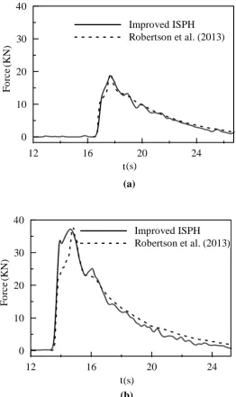
The ISPH computed time histories of wave impact forces on the wall by using the mixed source term formulation Eq. (14) are compared with the experimental data of Robertson et al. (2013) in Figs. 6 (a) and (b), for the initial wave height of H = 53.2 cm and 106.4 cm, respectively. It is shown that each time history is characterized by a rapid increase in the force load to the maximum, which is the result of direct wave collision with the solid wall and the subsequent climbing up of the water. The increase is much more obvious in the larger wave height case than the smaller one. As to the maximum wave force arrival time, it is t =

25.9m 28.5m

2.66m Water

1:12

15

17.67 s for the smaller wave and t = 14.63 s for the larger wave. Here it should be noted that the time origin in the present ISPH and that in Robertson et al. (2013) was different. The former was defined at the start of the solitary wave propagation, while the latter was defined when the wave impact started. After the wave forces reached their peak values, they started to decrease slowly due to the running down of the flow. A reflective bore also formed travelling away from the wall and thus the residual force loads dissipated over the time.

Fig. 6 Time histories of computed wave forces by ISPH and experimental data of

Robertson et al. (2013). (a) Wave height 53.2 cm; (b) Wave height 106.4 cm

t

F

o

rc

e

12 16 20 24

0 10 20 30 40

Improved ISPH Robertson et al. (2013)

(K

N

)

(s)

(a)

t

F

o

rc

e

12 16 20 24

0 10 20 30 40

Improved ISPH Robertson et al. (2013)

(K

N

)

(s)

16

Fig. 6 shows that the ISPH computations agreed quite satisfactorily with the experimental data of Robertson et al. (2013) in that both the force amplitude and evolution feature are well reproduced. However, relatively large errors appeared in case of the larger wave height of H = 106.4 cm during the violent wave impact. The experimental data exhibited a monotonous increase in the measured forces before the peak with a narrow peak zone, while the ISPH predicted a much wider peak force zone and also the force curve has double peaks during the wave impact around time t = 14.5 s, in spite that the first small peak is not very distinguishable. This first small force peak happened just a little earlier than the second and much larger peak. Although this phenomenon needs to be further investigated, it is believed to be caused by the nonlinear nature of the wave. The present solitary wave has a height-depth ratio of 0.4, thus it is highly nonlinear. It has been previously reported that the smaller amplitude solitary waves can impact on the solid wall with a single force peak, while the larger amplitude solitary waves can generate two force peaks due to the nonlinear wave dynamics (Cooker et al., 1997).

17

x

y

0 10 20 30 40 50 60 70 80

0 3 6 9

0 6250 12500 18750 25000 =2s (Pa) t (m) (m ) P x y

0 10 20 30 40 50 60 70 80

0 3 6

0 6250 12500 18750 25000 =4s t (m) (m ) x y

0 10 20 30 40 50 60 70 80

0 3

6 t=7.2s

(m)

(m

)

x

y

0 10 20 30 40 50 60 70 80

0 3 6

0 6250 12500 18750 25000 =9s t (m) (m ) x y

0 10 20 30 40 50 60 70 80

0 3 6

0 6250 12500 18750 25000 =13.8s t (m) (m ) x y

0 10 20 30 40 50 60 70 80

0 3 6

0 6250 12500 18750 25000 =14.2s

t

(m)

(m

18

Fig. 7 ISPH computed particle snapshots with pressure contours at different times

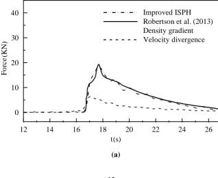
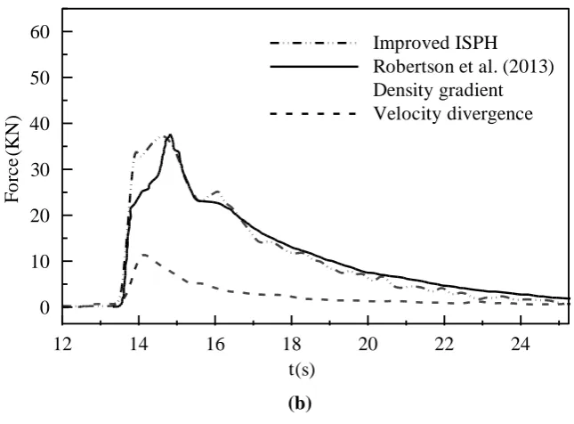
To evaluate the performance of different PPE source term treatments in ISPH for the wave force prediction, the density-invariant source term Eq. (10) and velocity divergence-free source term Eq. (13) are separately used to re-compute the time histories of wave impact forces on the right wall based on the same computational setting. The results are shown in Figs. 8 (a) and (b), for the wave height of 53.2 cm and 106.4 cm again, respectively. Meanwhile, the mixed source term results based on Eq. (14) and experimental data of Robertson et al. (2013) are also shown for a comparison. It can be seen that the computed wave forces follow the same trend as the wave impact pressures in the previous dam break simulation, in that the pure density-invariant model predicted a higher and more fluctuating force evolution while the pure divergence-free model predicted a smaller and smoother force evolution, but the ranges of over- and under- predictions are much less than those in the dam break flow due to the integration of pressures, which have greatly reduced the large fluctuations. For both wave heights, the pure density-invariant ISPH model overestimated the peak wave forces by 55% ~ 60%, while the pure divergence-free ISPH model under-predicted the peak forces by 65% ~ 70%.

x

y

0 10 20 30 40 50 60 70 80

0 3 6

0 6250 12500 18750 25000 =15.8s

t

(m)

(m

)

t

F

o

rc

e

12 14 16 18 20 22 24 26

0 10 20 30

40 Improved ISPH

Robertson et al. (2013) Density gradient Velocity divergence

(K

N

)

(s)

19

Fig. 8 Time histories of computed wave forces (on solid wall) by three different ISPH source terms and compared with experimental data of Robertson et al. (2013). (a) Wave

height 53.2 cm; (b) Wave height 106.4 cm

Comparison with WCSPH for another Dam Break Flow

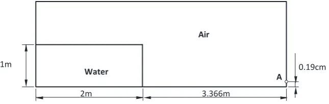
As recently found in some SPH studies (Hughes and Graham, 2010; Chen et al. 2013), the WCSPH could perform better in the fluid impact simulations in view of obtaining more stable and smoother pressure fields. To investigate this, in this section we consider another benchmark dam break problem for which a wide range of WCSPH results are available. Here the dam break flow as described by Colagrossi and Landrini (2003) is studied. The initial column of water covered a rectangular dimension of 2 m wide and 1 m high, and the right wall of the numerical tank is positioned 5.366 m from the left wall. A schematic view of the numerical tank is shown in Fig. 9. Adami et al. (2012) used the WCSPH with improved solid boundary treatment to compute the impact pressure measured in the bottom region of the right wall. An initial particle spacing of X = 0.01 m was used in their simulations. On the other hand, Marrone et al. (2011) used a novel  -SPH scheme based on the addition of a numerical diffusion term into the continuity equation with an initial particle spacing X = 0.015 m ~ 0.001875 m. Here we will compare our ISPH results computed by using the PPE source term Eq. (14) with these two WCSPH solutions to show the robustness of the mixed source term formulation.

t

F

o

rc

e

12 14 16 18 20 22 24

0 10 20 30 40 50 60

Improved ISPH Robertson et al. (2013) Density gradient Velocity divergence

(K

N

)

(s)

20

Fig. 9 Schematic view of numerical tank for dam break flow (Colagrossi and Landrini, 2003)

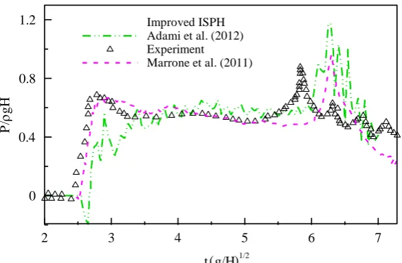
For a quantitative validation, in Fig. 10 we compare the temporal pressure profiles on the downstream wall for three different ISPH results and the experimental data of Buchner (2002). It is shown that the pressure profile obtained with Adami et al. (2012) contained some high frequency oscillations although the main pressure plateau was reasonably captured. According to Adami et al. (2012), the strong pressure peak around t(g/H)1/2 = 6 was caused by the plunging wave rolling-up after the flow hit upon the wall, but the numerical peak occurred slightly later because the air cushion effect was not considered in their single phase simulations. However, it should be noted that Adami et al.’s (2012) results were obtained without the implementations of XSPH and density normalization. Thus it can be compared on an equal basis with the present ISPH model in which no additional numerical smoothing techniques were used. The ISPH results in Fig. 10 indicated that the mixed source term formulation provided a very promising pressure time history, in that not only the pressure noises were reduced but also several smaller pressure peaks after time t(g/H)1/2 = 6 as observed in the experiment of Buchner (2002) were also well captured. Although the largest pressure peak was still delayed in the ISPH computation, the amplitude of pressure has been much better reproduced as compared with Adami et al. (2012). On the other hand, we have to admit that the ISPH computations are poorer than the  -SPH results of Marrone et al. (2011) until time t(g/H)1/2 = 6, which was due to that the latter model included more advanced numerical treatments by including the artificial diffusive term into continuity equation to remove the spurious high-frequency pressure oscillations. Nonetheless, Marrone et al. (2011) only reproduced the largest pressure peak around time 1/2

) / (g H

t = 6.35 (based on their particle spacing X = 0.015 m) and then the pressure curve drastically dropped down. In contrast, the ISPH computation also found two subsequent smaller pressure peaks that were reported in the experimental data. Besides, we should realize that Marrone et al. (2011) had reproduced these small pressure peaks by using very refined particle spacing X = 0.001875 m, while the present ISPH model achieved similar results by using X = 0.02 m.

2m

1m _0.19cm

A Water

3.366m

21

Fig. 10 Time histories of computed pressures by present ISPH, modified WCSPH (Adami et al., 2012),  -SPH (Marrone et al., 2011) and compared with experimental

data of Buchner (2002)

Numerical Error Analysis of Different Source Term Treatments

The preceding model applications have served to demonstrate that the mixed source term ISPH model performed much more promisingly than the corresponding source term model by using either a density-invariant or a velocity divergence-free formulation. In this section, we will carry out a series of numerical error analysis to investigate the PPE source term errors and provide a theoretical rational for the robustness of the mixed source term formulation.

Generally there are two main errors arising from any ISPH projection schemes and they are the particle density error and the velocity divergence error. The former is due to the change of particle volume from either the compression or expansion, while the latter is attributed to the non-conservation of the particle flow field. In a pure density-invariant ISPH approach such as in Shao and Lo (2003), we would expect that the conservation of particle volume is well observed, but in a pure divergence-free ISPH approach such as in Cummins and Rudman (1999), we would expect that the conversation of particle velocity field is well followed. As far as the present knowledge is concerned, only a limited number of works have been carried out to study the particle density errors in ISPH projection scheme, such as documented by Cummins and Rudman (1999), Asai et al. (2012) and Szewc et al. (2012). However, with regard to the evaluation of particle velocity divergence errors there are no

t g/H

P

/



g

H

2 3 4 5 6 7

0 0.4 0.8

1.2 Improved ISPH Adami et al. (2012) Experiment

Marrone et al. (2011)

22

documented results available. In fact, the understanding of these fundamental errors would be very useful for understanding and improving the ISPH numerical schemes, as they could greatly influence the model predictions of the macro flow properties such as the impact pressure and force, etc.

In the following error analysis, the particle density error is quantitatively evaluated through the normalized density errors between the corrected and initial constant densities as:



 

'

1

0 0

' ( ) /

1 ) (

N

i i

den t

N t

E    Eq. (21)

where the search of neighbouring particles includes the inner fluid particles only. For the velocity divergence error, it is quantified through the average divergence values of corrected particle velocities as



  

'

1

' ( )

1 ) (

N

i

i

div t

N t

E u Eq. (22)

Numerical Errors in Temporal Domain

Based on the numerical simulations in the previous dam break flow of Lee et al. (2011),

23

mixed source term formulation improved the volume conservation of fluid particles and thus made the computation more stable.

(a)

(b)

Fig. 11 Time histories of errors from different source term formulations (for dam break flow of Lee et al., 2011): (a) Density error; (b) Velocity divergence error

t

Ed

en

0.5 1 1.5 2 2.5 3

0 0.08 0.16 0.24

0.32 Mixed source term

Density gradient Velocity divergence

(s)

t

Ed

iv

0 0.5 1 1.5 2 2.5 3

1 2 3 4 5

Mixed source term Density gradient Velocity divergence

(s)

(s

24

On the other hand, examining the velocity divergence errors in Fig. 11 (b) reveals that a strict density-invariant ISPH formulation could generate relatively large divergence errors while a strict divergence-free ISPH formulation could reduce this error by about 50%. It is interesting to notice that the fluctuation features of divergence errors in Fig. 11 (b) are quite consistent with those of the density errors in Fig. 11 (a), in that the peak errors appear around the same time instants when the flows are undergoing the severe impacts and free surface deformations. However, it is also found out that the divergence errors in Fig. 11 (b) appear to be similar for both the mixed source term model and the pure divergence-free model. The reason is likely to be that the density and divergence errors are internally interrelated with each other. In a strict divergence-free model, as the particle volume conservation is not satisfied as shown in Fig. 11 (a), this could also influence the correct projection of the particle velocity fields. Thus the simple imposition of divergence-free condition alone in a particle method cannot achieve the best divergence-free flow field, which is different from the grid modelling technique. In comparison, in the mixed source term model, as the particle volume conservation is improved and the density error is reduced, this can also make the projection of particle velocity field more accurate. As a result, the mixed source term ISPH scheme achieved the same velocity divergence errors as the pure velocity divergence-free model.

As a further investigation on the different source term formulations, the time histories of the particle density and velocity divergence errors are determined as shown in Figs. 12 (a) and (b), for the three source terms as represented by Eqs. (10), (13) and (14), based on the previous numerical simulations of dam break flow of Colagrossi and Landrini (2003). Besides, similar results are also presented for the solitary wave impact case of Robertson et al. (2013) in Figs. 13 (a) and (b), for the small wave height of 53.2 cm.

(a) t

Ed

en

0.5 1 1.5 2 2.5 3 3.5 4

0 0.08 0.16 0.24

0.32 _{Mixed source term}

Density gradient Velocity divergence

25

(b)

Fig. 12 Time histories of errors from different source term formulations (for dam break flow of Colagrossi and Landrini, 2003): (a) Density error; (b) Velocity divergence error

(a)

t

Ed

iv

0 0.5 1 1.5 2 2.5 3 3.5 4

1 2 3 4 5

Mixed source term Density gradient Velocity divergence

(s)

(b)

(s

-1 )

t

Ed

en

12 16 20 24

0 0.1 0.2 0.3 0.4 0.5

Mixed source term Density gradient Velocity divergence

26

(b)

Fig. 13 Time histories of errors from different source term formulations (for solitary wave impact of Robertson et al., 2013): (a) Density error; (b) Velocity divergence error

Fig. 12 showed the same error features as those in Fig. 11, in that the mixed source term model achieved the most optimum numerical performance in view of reducing the density and divergence errors, and also the two errors are consistent with each other for the appearance of peak values. In fact this is of no surprise as both cases are for the instantaneous dam break flows and thus should have similar hydrodynamic mechanisms. On the other hand, the density and divergence errors of solitary wave impact as shown in Fig. 13 have somewhat different evolution patterns. For example, Fig. 13 (a) demonstrated that the density error for a pure divergence-free source term formulation could be as large as 45% in a long time simulation, while Fig. 13 (b) indicated that the divergence error for the mixed source term lies somewhere between that of the pure density-invariant and divergence-free models, rather than close to the latter as in the two dam break flow cases. At this stage we could only attribute this discrepancy to the different hydrodynamic features of the flow and the duration of simulation time. However, a very promising phenomenon observed is that both the dam break flows and solitary wave impact shared some similar features such as: (1) the mixed source term could achieve the optimum density and divergence errors simultaneously; (2) the peak density and divergence errors always appear during the violent fluid motions such as wave impact. For example, in the solitary wave case, the maximum density and divergence errors both occurred around time t = 18 s as shown in Fig. 13, while in the violent wave impact case they happened at t = 17.67 s as shown in Fig. 6 (a).

t

Ed

iv

12 16 20 24

0 0.1 0.2 0.3 0.4 0.5

Mixed source term Density gradient Velocity divergence

(s)

(b)

(s

27

Numerical Errors in Spatial Domain

In the preceding analysis, we found that relatively large density and velocity divergence errors are always associated with the rapid flow deformation and impact. To numerically support this statement here we further examine the spatial distribution of these errors for the dam break flow of Lee et al. (2011), during the violent flow impact on the right wall. Figs. 14 (a) and (b) showed the density and divergence errors for the mixed source term model Eq. (14), while (c) is the density error for the density-invariant model Eq. (10) and (d) is the velocity divergence error for the divergence-free model Eq. (13), respectively.

(a) (b)

(c) (d)

Fig. 14 Spatial distributions of errors from different source term formulations (for dam break flow of Lee et al., 2011): (a) Density error for mixed source term; (b) Velocity divergence error for mixed source term; (c) Density error for density-invariant model;

(d) Velocity divergence error for divergence-free model x

y

0 0.5 1 1.5

0 0.3 0.6 0.9 1.2

-0.3 -0.15 0 0.15 0.3

(m) (m ) Density error x y

0 0.5 1 1.5

0 0.3 0.6 0.9 1.2

-5 -2.5 0 2.5 5 =0.47s t (m) (m ) Divergence x y

0 0.5 1 1.5

0 0.3 0.6 0.9 1.2

-0.3 -0.15 0 0.15 0.3 =0.46s t (m) (m ) Density error x y

0 0.5 1 1.5

0 0.3 0.6 0.9 1.2

28

Figs. 14 clearly demonstrate that large density and divergence errors are concentrated within the impact region near the right wall, especially around the upward flowing jet where the water surface undergoes large deformation. Besides, some of the larger density and divergence errors are also found on the free surface particles across the computational domain. In comparison, these errors are quite small within the inner fluid region away from the solid boundary and free surface.

In some earlier results, we have observed that the velocity divergence errors in the pure divergence-free source term model may have arisen from the particle volume conservation. To provide a rational for this, Figs. 15 (a) and (b) showed the spatial plot of particle density errors at the time when the velocity divergence error is large, for the divergence-free source term Eq. (13) model and mixed source term Eq. (14) model, respectively. The result is based on the dam break flow of Colagrossi and Landrini (2003) at the stage when the flow overturned from the right wall and plunged onto the water surface at normalized time

2 / 1

) / (g H

t = 6.25 as shown in Fig. 10. Figs. 15 (a) showed that for a pure divergence-free source term model the density error or particle volume non-conservation is obviously larger especially within the impact region near the solid boundary, while these errors have been effectively reduced in the mixed source term model as shown in Figs. 15 (b).

(a)

(b)

Fig. 15 Spatial distributions of density errors (for dam break flow of Colagrossi and Landrini, 2003) for (a) Divergence-free source term and (b) Mixed source term

x

y

0 1 2 3 4 5

0 0.5 1 1.5 2

-0.3 0 0.3

(m)

(m

) Density error

x

y

0 1 2 3 4 5

0 0.5 1 1.5 2

-0.3 0 0.3

(m)

(m

29

Finally, to further investigate why the velocity divergence error is large for the density gradient source term, the spatial plots of the velocity divergence errors and pressure fields for the dam break flow of Lee et al. (2011) during the flow impact on the right wall are shown in Figs. 16 (a) and (b), respectively, for the density-invariant source term Eq. (10) model. Figs. 16 (a) demonstrated a noisy divergence field that is closely correlated with the noisy pressure and velocity distribution patterns near the dam site as well as impact zone, as shown in Figs. 16 (b).

(a)

(b)

Fig. 16 Spatial distributions of (a) Velocity divergence errors and (b) Pressure and velocity fields, for density-invariant source term model (for dam break flow of Lee et al.,

2011) x

y

0 0.5 1 1.5

0 0.3 0.6 0.9 1.2

-5 -2.5 0 2.5 5

(m)

(m

)

Divergence

x

y

0 0.5 1 1.5

0 0.3 0.6

0.9 8000

6000 4000 2000 0

(m)

(m

)

30

Conclusions

To improve the ISPH modelling capacity a mixed source term model has been proposed by the authors which combines the standard density-invariant and the velocity divergence-free formulations in a weighted average form. The new model was applied to two benchmark dam break flows and one solitary wave impact problem for two different wave heights. By comparing with the documented experimental data and numerical results, it was found that the mixed source term ISPH model predicted more accurate impact pressure and force as compared with the results obtained by using either the density-invariant or the velocity divergence-free ISPH model.

To further quantify the numerical errors generated from different ISPH source term treatments, the temporal and spatial distributions of the particle density and velocity divergence errors were investigated. Not only we have found that the numerical errors were closely linked with the violent fluid deformation and impact, but also it has been disclosed that a strict density-invariant model could generate relatively larger divergence error while a strict divergence-free model could generate relatively larger density error. The mixed source term model can effectively reduce both errors in an optimum manner and thus gave the best numerical performance in predicting the macro flow behaviours.

Acknowledgements

31

References

Adami, S., Hu, X.Y. and Adams, N.A. (2012), A generalized wall boundary condition for smoothed particle hydrodynamics, Journal of Computational Physics, 231, 7057-7075.

Asai, M., Aly, A.M., Sonoda, Y. and Sakai, Y. (2012), A stabilized incompressible SPH method by relaxing the density invariance condition, Journal of Applied Mathematics, 2012, Article ID 139583.

Buchner, B. (2002), Green Water on Ship-type Offshore Structures, Ph.D. Thesis, Delft University of Technology.

Chang, T. J. and Chang, K. H. (2013), SPH modeling of one-dimensional nonrectangular and nonprismatic channel flows with open boundaries, Journal of Hydraulic Engineering, ASCE, 139(11), 1142-1149.

Chen, Z., Zong, Z., Liu, M.B. and Li, H.T. (2013), 2A comparative study of truly incompressible and weakly compressible SPH methods for free surface incompressible flows, Int. J. Numer. Meth. Fluids, 73, 813–829.

Chorin, A.J. (1968), Numerical solution of the Navier-Stokes equations, Math. Comp, 22(104), 745–762.

Colagrossi, A. and Landrini, M. (2003), Numerical simulation of interfacial flows by smoothed particle hydrodynamics, Journal of Computational Physics, 191, 448–475.

Cooker, M.J., Weidman, P.D. and Bale, D.S. (1997), Reflection of a high-amplitude solitary wave at a vertical wall, J. Fluid Mech., 342, 141–158.

Crespo, A. J. C., Gómez-Gesteira, M. and Dalrymple, R. A. (2007), Boundary conditions generated by dynamic particles in SPH methods, CMC, 5(3), 173-184.

Cummins, S.J. and Rudman, M. (1999), An SPH projection method, Journal of Computational Physics, 152(2), 584-607.

Gómez-Gesteira, M., Cerqueiro, D., Crespo, C. and Dalrymple, R.A. (2005), Green water overtopping analyzed with a SPH model, Ocean Eng, 32(2), 223-238.

32

Gui, Q., Shao, S. and Dong, P. (2014), Wave impact simulations by an improved ISPH model, J. Waterway, Port, Coastal, Ocean Eng., ASCE, 140(3), 04014005.

Hu, X.Y. and Adams, N.A. (2007), An incompressible multi-phase SPH method, Journal of Computational Physics, 227(1), 264-278.

Hughes, J. and Graham, D. (2010), Comparison of incompressible and weakly-compressible SPH models for free-surface water flows, Journal of Hydraulic Research, 48(Extra Issue), 105–117.

Khayyer, A. and Gotoh, H. (2009), Modified Moving Particle Semi-implicit methods for the prediction of 2D wave impact pressure, Coastal Engineering, 56(4), 419-440.

Khayyer, A. and Gotoh, H. (2011), Enhancement of stability and accuracy of the moving particle semi-implicit method, Journal of Computational Physics, 230(8), 3093-3118.

Khayyer, A. and Gotoh, H. (2012), A 3D higher order Laplacian model for enhancement and stabilization of pressure calculation in 3D MPS-based simulations, Applied Ocean Research, 37, 120– 126.

Khayyer, A., Gotoh, H. and Shao, S. (2009), Enhanced predictions of wave impact pressure by improved incompressible SPH methods, Appl Ocean Res, 31(2), 111-131.

Koh, C.G., Luo, M., Gao, M. and Bai, W. (2013), Modelling of liquid sloshing with constrained floating baffle, Computers and Structures, 122, 270–279.

Lee, E.S., Moulinec, C., Xu, R., Violeau, D., Laurence, D. and Stansby, P. (2008), Comparisons of weakly compressible and truly incompressible algorithms for the SPH mesh free particle method, Journal of Computational Physics, 227(18), 8417-8436.

Lee, B.H., Park, J.C., Kim, M.H. and Hwang, S.C. (2011), Step-by-step improvement of MPS method in simulating violent free-surface motions and impact-loads, Comput. Methods Appl. Mech. Engrg., 200, 1113–1125.

Liu, X., Xu, H., Shao, S. and Lin, P. (2013), An improved incompressible SPH model for simulation of wave–structure interaction, Computers & Fluids, 71, 113-123.

Lucy, L. (1977), A numerical approach to the testing of the fission hypothesis, The Astronomical Journal, 82, 1013–1024.

Marrone, S., Antuono, M., Colagrossi, A., Colicchio, G., Le Touzé, D. and Graziani, G.

(2011), -SPH model for simulating violent impact flows, Comput. Methods Appl. Mech.

33

Monaghan, J.J. (1992), Smoothed Particle Hydrodynamics, Annu Rev Astron Astr, 30(1), 543-574.

Monaghan, J.J. and Kajtar, J.B. (2009), SPH particle boundary forces for arbitrary boundaries, Computer Physics Communications, 180(10), 1811-1820.

Monaghan, J.J., Kos, A. and Issa, N. (2003), Fluid motion generated by impact, J. Waterway, Port, Coastal, Ocean Eng., ASCE, 129(6), 250-259.

Robertson, I.N., Paczkowski, K., Riggs, H.R. and Mohamed, A. (2013), Experimental investigation of Tsunami bore forces on vertical walls, Journal of Offshore Mechanics and Arctic Engineering, ASME, 135, 021601-1.

Shadloo, M.S., Zainali, A., Yildiz, M. and Suleman, A. (2012), A robust weakly compressible SPH method and its comparison with an incompressible SPH, Int. J. Numer. Meth. Engng, 89, 939–956.

Shao, S. and Lo, E.Y.M. (2003), Incompressible SPH method for simulating Newtonian and non-Newtonian flows with a free surface, Advances in Water Resources, 26(7), 787-800.

Szewc, K., Pozorski, J. and Minier, J.-P. (2012), Analysis of the incompressibility constraint in the smoothed particle hydrodynamics method, Int. J. Numer. Meth. Engng, 92, 343–369.

Vacondio, R., Rogers, B. D., Stansby, P. K. and Mignosa, P. (2013), Shallow water SPH for flooding with dynamic particle coalescing and splitting, Advances in Water Resources, 58, 10–23.

Xia, X. L., Liang, Q. H., Pastor, M., Zou, W. L. and Zhuang, Y. F. (2013), Balancing the source terms in a SPH model for solving the shallow water equations, Advances in Water Resources, 59, 25–38.