International Journal of Innovative Technology and Exploring Engineering (IJITEE) ISSN: 2278-3075, Volume-9 Issue-2S, December 2019
Abstract: Customer churn prediction has always been a major problem in telecom industries. Customer retention is always one of the major objectives of any service providing company as maintaining loyal customers has always been cheaper than acquiring new customers. In this paper, we have tried to predict the churn rate of a dataset from a telecom company using some classifiers and then training the same classifiers with ensemble learning models. The ensemble techniques are assumed to yield better results. We have used 42 classifiers from over different like Nearest Neighbors, Decision Tables, Random Forests, etc., which roughly covers almost all the well-known classifiers used in the industry in today’s date. Further, the ensemble techniques are used in our work such as bagging and boosting which are trained on the same classifiers so that we can compare the performance of individual classifiers as well as the same when used as a base classifier. We have extracted the accuracy of the classifiers, True Positive and False Positive rates, f-measure, MCC score, Area Under Curve (AUC) area and Precision-Recall (PRC) area. These measures, not only helped us know which algorithm is more fruitful but also gave us insights about the varying performance. It is observed that, in most of the cases, the classifiers, when combined with either of the ensemble techniques, yield better results. The experimental results reveal that the accuracy of the classifier improves when combined with bagging or boosting.
Keywords: Churn Prediction, Bagging, Boosting, Machine Learning.
I. INTRODUCTION
I
n today’s situation of intense competition between companies for building, finessing and strengthening loyal and long-lasting relationships, retaining customers is one of the key objectives for the companies. The essentialness of this objective is obvious, given the fact that first, acquiring a new customer can cost 5 times more than retaining an already existing customer. Second, an increment in customer retention by 5% results in profit increment of 25-95% and, third, the success rate with an existing customer is thrice than that of a new customer [1]. Thus, any toolkit or language which can give insights to or predict the retention percentage plays a really significant role in Business Intelligence. The technical term used in the industry for this is ‘Churn’ which means the discontinuation of a contract [2]. Industries like telecommunication industry, banking [3], insurance companies, and gaming [4]-[5] are the areas where churn is a major problem, and in the last few decades, there has been a huge surge in relative studies. Although churn is anRevised Manuscript Received on December 12, 2019. * Correspondence Author
D. A. Debjyoti, M. Tech scholar of CSE Dept., NIT Arunachal Pradesh, Yupia, Arunachal Pradesh, India. Email: [email protected]
G. Deepak*, Assistant Professor of CSE Dept., NIT Arunachal Pradesh, Yupia, Arunachal Pradesh, India. Email: [email protected]
unavoidable phenomenon, considering certain behaviors can help us find the reason and hence reduce this problem.
In the field of predictive analytics, whenever a researcher has to develop a churn model, they usually select the classifier which they ‘believe’ will yield the best results. This belief is generally due to the partial knowledge about the available classifiers. Apart from these ‘classical’ classifiers, there exists a separate family of classifiers named as ‘Meta Classifiers’ [6]. These Meta classifiers train over a batch of classical classifiers and build a model which is observed to be better than the latter one when applied individually. Two such techniques are used in our work which is Bagging and Boosting to train the same classifiers.
Our work consists of predicting churn rate using a widely used data mining toolkit called Weka [7]. Further, the final comparative analysis is done on python.
II. RELATED WORK
Churn Prediction using machine learning has been a very popular research field among data scientists from over a decade. Researchers have been targeting this field not only to give insights and beneficiate the industries but also to experiment on it with their new classification models. In 2007, Zhao et al., used their improved support vector machine (SVM) algorithm to perform churn analysis [8]. Three years later, Lima et al., produced a case study over integrating the domain knowledge in the field of data mining using decision tables [9]. In the following decade, there has been a huge surge in this field, in 2011, Bock et al., gave an empirical evaluation of several variations of rotation based ensemble techniques [10]. Further, in 2013, Hashmi et al., wrote a review paper exploring the works done on different applications in this field [11]. In the following year, Adwan et al., used multilayer perceptron to predict churn ratio in telecom industry [12]. This was the same period from when industry witnessed the increase in popularity of deep learning techniques in churn prediction. In the same year, the contribution of Castanedo et al., with their research on churn prediction using deep learning techniques [13] reflects how advances techniques helped us to get better results. In 2017, Hashmi et al., used this field to experiment with their new proposed decision making technique using rough-set-theory [14]. In 2018, Caigny et al., proposed a new hybrid technique and used this for churn prediction [15]. One can observe the change in this field over the last 2 decades and how the innovation in the machine learning techniques helps in overall performance improvement of churn prediction.
Ensemble Learning Models for Churn Prediction
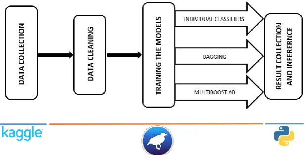
Fig. 1 Skeletal Architecture of the methodology used in our work
III. METHODOLOGY
This section will be in two parts. Firstly, we cover all the details about the dataset and experiment setup and further followed by the explanation and details about the method, we used to apply the classifiers, both classical as well as the ensembles. The flowchart given in Figure 1 explains the architecture of the methodology we use.
The basic structure we follow is:- Step 1: Data collection.
Step 2: Cleaning the data by removing unimportant features such as customer id, etc.
Step 3: Training the 42 classifiers by using a 4-fold Cross Validation technique.
Step 4: Extracting the results generated in Step 3 using python and converting it into CSV format.
Step 5: Calculating relevant features using python. The following sections explain the above mentioned steps in detail.
A. Dataset and experiment setup
In our work, we have selected a dataset from the Teradata center for Customer Relationship Management at Duke University, February 2014 [16]. The dataset consists of 49752 customers with 55 attributes out of which one is our target label. The exploratory data analysis reveals that out of 49752 customers, 14245 customers decided to unsubscribe from the company’s service or ‘churned out’. We have found that the ratio of non-churn to churn is 2.49. Hence, we can see that the data is unbalanced.
We use Weka 3.8.3 [7] to perform our experiment. It is observed that fitting the data and preparing them for the classifiers is easier. Weka saves the data in its own type of file with arff (Attribute Retention File Format) extension which can be later imported for any experiments. This software has in built stratified cross-validation method for the data preparation and a 4-fold cross-validation is used in our experiment. We use Weka’s explorer framework as it provides more statistics about the performance of the classifiers.
Apart from the above mentioned operations, no other pre-processing is done on the dataset. We chose to conduct our experiment on as much crude data as possible so as to
reduce any sort of bias that could result on different classifiers. Final analysis of the acquired results and visualization of the derived output was done on the language Python [17].
B. Models for churn prediction
i) Individual classifiers without bagging or boosting
The following classifiers are implemented on Weka 3.8.3 (Explorer framework). The data is first converted to Weka’s arff format which is later used with all the experiments. The dataset have all the attributes’ type as numeric except the target attribute. The type of target label is set as ‘nominal’. 1.Decision Stump [18]
A decision stump is a classifier which consists of single-level decision tree, in other words, the tree consists of just root and leaf levels. This performs classification based on the entropy of the attributes.
This classifier is trained after tuning the parameter batchSize set as 100.
2.Decision Table [19]
This classifier builds a simple decision table which makes the decision using maximum voting technique.
We set the parameters batchSize to a 100 and the search method to ‘Best First Search’ method.
3.HyperPipes [20]
This classifier creates HyperPipes for every category which stores all the points of that particular category. All the parameters are set to default for this classifier. 4.IBk [21]
IBk is the K-nearest neighbor algorithm for classification. It predicts the output of an unknown data by comparing its distance with ‘k’ neighbors.
We set the number of nearest neighbors to 1. Further the nearest neighbor would be searched by following Euclidian’s algorithm to find distance between 2 points. 5.J48 [22]
This classifier creates pruned or unpruned C4.5 decision trees.
The confidence factor is set to 0.25, with 2 instances per leaf and numFold to 3.
6.LibSVM [23]
LibSVM stands for libraries of SVM. This contains several types of SVM like One-Class, Regressing, nu-SVM are supported in this, with the
International Journal of Innovative Technology and Exploring Engineering (IJITEE) ISSN: 2278-3075, Volume-9 Issue-2S, December 2019
[image:3.595.54.547.90.236.2]with the kernel’s degree set to 3. Further, to implement this, we set the batchSize to 100.
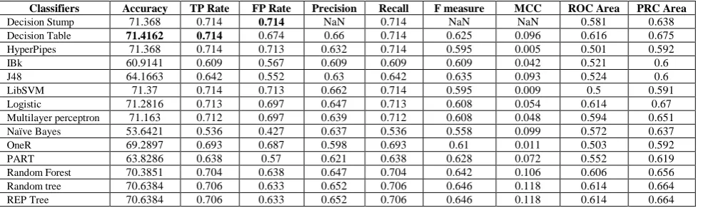
Table I. Performance measures of the classifiers when applied without any ensemble technique
7.Logistic [24]
This classifier builds a multinomial logistic regression model having a ridge estimator.
In order to train the model on the software, we set the ridge parameter to log-likelihood of 10-8. The classifier capabilities are checked before the classifier was built. 8.MultiLayer Perceptron [25]
This classifier uses back propagation to train a multilayer perceptron for classification. This network can be hand coded as well but Weka’s tailored GUI helped us to create the network by specifying the parameters.
The batchSize is used to train this classifier as 100, with learning rate tuned at 0.3, momentum of 0.2 and a validation Threshold of 20.
9.Naïve Bayes [26]
This classifier uses estimator classes. After analyzing the training data, the values of numeric estimator precision values are determined.
The parameter kernelEstimator for numeric attributes is set to False for this classifier.
10.OneR [27]
This classifier makes its prediction by using the attribute having minimum error, converting numeric attributes to discrete values.
The batchSize used for this classifier is 100 and the minimum bucket size for discretizing the numeric attributes is 6.
11.PART [28]
This classifier generates a decision list using separate-and-conquer. In every iteration a C4.5 decision tree is built and the leaf with “best performance” is used to define the rule.
The confidence factor parameter, for training this classifier on Weka, is set to 0.25 and the number of folds used is 3.
12.Random Forest [29]
This classifier builds a forest of random trees.
For training this model, the bagSizePercent parameter and the number of iterations is set to 100.
13.Random Tree[30]
This classifier constructs a tree by considering K attributes chosen randomly for every node without performing any pruning. The minimum total weight of the instances in each leaf is set to 1 and the minVarianceProp parameter is set to 0.001, which decides the minimum proportion of the
variance on all the data that should be present at a node for the splitting.
14.REP Tree[31]
Abbreviation for Reduced Error Pruning Tree, this classifier is considered to be a fast decision tree learner. This classifier builds a decision tree using information gain and then prunes it using back fitting reduced-error pruning.
For training this classifier, the minimum total weight of instances in the leaves is set to 2, the minVarianceDrop is the same as that of the previous classifier.
ii) Individual Classifier with bagging
Bagging classifier [32] generates multiple versions of the same model and uses them to get an aggregated predictor with low variance. While predicting an output of an unknown data, the aggregated models choose voting technique to make the decision.
For training the Bagging Classifier on Weka we set the maximum batchSize to 100 with 10 iterations and a seeding value of 1.
iii) Individual Classifier with Boosting
MultiBoosting [33] is the successor of the very popular ensemble technique AdaBoosting [34]. This classifier is said to be the combination of the latter and the wagging classifier. MultiBoosting has both the advantages of AdaBoosting’s high bias and wagging’s higher variance reduction.
In order to train a MultiBoostAB Classifier on Weka we tune the parameters as same as that of the Bagging classifier with the batchSize, number of iterations and seeding value to 100, 10 and 1 respectively.
IV. ANALYSIS
Weka’s inbuilt feature allowed us to save the result generated into separate files. While calculating the performance measures, it often happened that the denominator is 0, consequently those measures could not be calculated. In such cases Weka’s version 3.7.3 returned a ‘?’. We replaced the ‘?’ with ‘NaN’ representing that they cannot be accounted. All the quality measures have their usual meaning in the context of machine learning. Since the class distribution is imbalanced, all the performance measures except the accuracy is given as
the weighted average of the output classes.
Classifiers Accuracy TP Rate FP Rate Precision Recall F measure MCC ROC Area PRC Area
Decision Stump 71.368 0.714 0.714 NaN 0.714 NaN NaN 0.581 0.638
Decision Table 71.4162 0.714 0.674 0.66 0.714 0.625 0.096 0.616 0.675
HyperPipes 71.368 0.714 0.713 0.632 0.714 0.595 0.005 0.501 0.592
IBk 60.9141 0.609 0.567 0.609 0.609 0.609 0.042 0.521 0.6
J48 64.1663 0.642 0.552 0.63 0.642 0.635 0.093 0.524 0.6
LibSVM 71.37 0.714 0.713 0.662 0.714 0.595 0.009 0.5 0.591
Logistic 71.2816 0.713 0.697 0.647 0.713 0.608 0.054 0.614 0.67
Multilayer perceptron 71.163 0.712 0.697 0.639 0.712 0.608 0.048 0.594 0.651
Naïve Bayes 53.6421 0.536 0.427 0.637 0.536 0.558 0.099 0.572 0.637
OneR 69.2897 0.693 0.687 0.598 0.693 0.61 0.011 0.503 0.592
PART 63.8286 0.638 0.57 0.621 0.638 0.628 0.072 0.552 0.619
Random Forest 70.3851 0.704 0.638 0.647 0.704 0.642 0.106 0.606 0.656
Random tree 70.6384 0.706 0.633 0.652 0.706 0.646 0.118 0.614 0.664
After getting the results of the performance from all the classifiers, the final analysis is done using python 3.7.3. All the results of different classifiers are stored in separate files, from which the relevant metrics are extracted using python’s package re (regular expression).
A. Performance measures of individual classifiers
Table I shows the performance of the individual classifiers. All the measures except the accuracy column are the combined weighted average of both the output classes. We have observed that the highest accuracy is produced while using Decision Table giving an accuracy of 71.41% with TP rate and FP rate of 0.714 and 0.674 respectively. We also noticed that the poorest performance is given by the classifier IBk with accuracy 60.91% and TP Rate and FP Rate of 0.609 and 0.567.
B. Performance measures of individual classifiers with Bagging technique
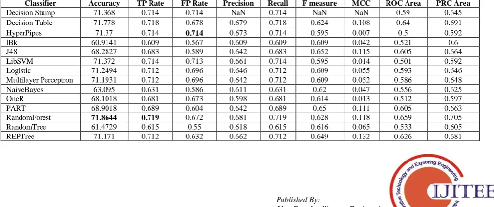
Table II shows the same measures as that of Table 1 but when the classifiers are trained with bagging. While using Bagging technique we observe a change in the best accuracy. With this technique, Random Forest produced the best accuracy of 71.91% with TP and FP rate 0.719 and 0.682. The classifier Decision Table, which gives the best result independently, when train as a base classifier for Bagging, give a less accuracy of 71.39%. Furthermore, we observe that the least accuracy is given by Naïve Bayes classifier.
C. Performance measures of individual classifiers with Boosting technique
Table III shows the performance measures resulted when the same classifiers are trained with MultiBoostAB. When trained with MultiBoostAB, we observe that the classifier RandomForest gives best results with an accuracy of 71.86%. We also observe that Decision Table which produce the best results when used individually, gives an increased accuracy of 71.778%, which even after being better than it’s individual performance, but it is still less than the best classifier. Furthermore, we notice that the classifier IBk produces the least accuracy of 60.91%.
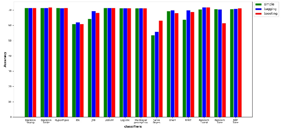
After applying the classifiers of all the 3 variants (individual, bagging and boosting), one can observe that there are some differences in the accuracies when we use Bagging or MultiBoostAB on the same algorithm. In order to visualize the same the following grouped bar graph in Fig. 1 represents the accuracies of the 3 variants of all classifiers. We have used python’s matplotlib (version 3.1.1) package to plot this graph. The data set is processed using the datatype called Pandas from the package of the same name. Further, in order to see the performance change, we calculated the difference in the accuracy of the classifiers with the ensemble techniques. Table IV shows the difference in the accuracy of the classifier with the ensemble techniques. Negative magnitude shows that the accuracy of the classifiers dropped when used with the ensemble technique whereas a positive magnitude would represent that using Bagging or Boosting actually improved the results of the classifier.
[image:4.595.45.551.428.579.2] [image:4.595.50.556.606.817.2]Table II. Performance measures of the classifiers when applied as base classifier with Bagging
Table III. Performance measures of the classifiers when applied as base classifier with MultiBoostAB
Classifier Accuracy TP Rate FP Rate Precision Recall F measure MCC ROC Area PRC Area
Decision Stump 71.368 0.714 0.714 NaN 0.714 NaN NaN 0.587 0.643
Decision Table 71.3941 0.714 0.712 0.698 0.714 0.596 0.024 0.614 0.673
HyperPipes 71.362 0.714 0.713 0.64 0.714 0.595 0.01 0.501 0.592
IBk 62.0156 0.62 0.574 0.611 0.62 0.615 0.048 0.532 0.61
J48 69.4826 0.695 0.597 0.649 0.695 0.656 0.128 0.619 0.675
LibSVM 71.37 0.714 0.713 0.661 0.714 0.595 0.01 0.501 0.592
Logistic 71.2896 0.713 0.697 0.648 0.713 0.608 0.055 0.614 0.67
Multilayer Perceptron 71.2434 0.712 0.697 0.645 0.712 0.608 0.054 0.616 0.67
NaiveBayes 55.9495 0.559 0.445 0.637 0.559 0.58 0.104 0.575 0.639
OneR 69.8103 0.698 0.693 0.599 0.698 0.607 0.011 0.507 0.596
PART 69.8103 0.698 0.693 0.599 0.698 0.607 0.011 0.507 0.596
RandomForest 71.9147 0.719 0.682 0.693 0.719 0.621 0.112 0.672 0.718
RandomTree 70.4333 0.704 0.643 0.646 0.704 0.64 0.102 0.602 0.653
REPTree 70.8132 0.708 0.62 0.658 0.708 0.653 0.134 0.635 0.69
Classifier Accuracy TP Rate FP Rate Precision Recall F measure MCC ROC Area PRC Area
Decision Stump 71.368 0.714 0.714 NaN 0.714 NaN NaN 0.59 0.645
Decision Table 71.778 0.718 0.678 0.679 0.718 0.624 0.108 0.64 0.691
HyperPipes 71.37 0.714 0.714 0.673 0.714 0.595 0.007 0.5 0.592
lBk 60.9141 0.609 0.567 0.609 0.609 0.609 0.042 0.521 0.6
J48 68.2827 0.683 0.589 0.642 0.683 0.652 0.115 0.605 0.664
LibSVM 71.372 0.714 0.713 0.661 0.714 0.595 0.014 0.501 0.592
Logistic 71.2494 0.712 0.696 0.646 0.712 0.609 0.055 0.593 0.646
Multilayer Perceptron 71.1931 0.712 0.696 0.642 0.712 0.609 0.052 0.586 0.648
NaiveBayes 63.095 0.631 0.586 0.611 0.631 0.62 0.047 0.556 0.625
OneR 68.1018 0.681 0.673 0.598 0.681 0.614 0.013 0.512 0.597
PART 68.9018 0.689 0.604 0.642 0.689 0.65 0.111 0.605 0.663
RandomForest 71.8644 0.719 0.672 0.681 0.719 0.628 0.118 0.659 0.705
RandomTree 61.4729 0.615 0.55 0.618 0.615 0.616 0.065 0.533 0.605
International Journal of Innovative Technology and Exploring Engineering (IJITEE) ISSN: 2278-3075, Volume-9 Issue-2S, December 2019
Fig.2 Grouped Bar Graph of all the classifiers with their Meta classifier counterparts
Table IV. Difference in the accuracies of Ensemble techniques and the individual classifiers
V. RESULTS
We have found that with the highest accuracy of 71.9%, bagging random forest has given the best result and predicted that 691 customers would ‘churn out’ of the services provided by the company. Further, it is found that when used with the Boosting technique, Random Forests again turned to be the best classifier with an accuracy of 71.8644% which is just 0.0503% less than the former ensemble technique. On the other hand, when we used individual classifiers, the Decision Table classifier turned out to be the best classifier giving out the accuracy of 71.4%. One can observe that this result is still less than the best result we have achieved when using ensemble techniques hence confirming the fact that using a meta classifier for this purpose is a better choice than using individual classifiers. We have also found that out of the 14 classifiers, on applying the Bagging technique, the accuracy of the classifiers Decision Table, HyperPipes and Random Tree dropped by 0.02, 0.006 and 0.2 percentages. On the other hand, on applying the Boosting technique the accuracy of Logistic, OneR and Random Tree dropped by
0.032, 1.18 and 9.16 percent respectively. The best improvement in the accuracy is given by the classifier PART with an increment of 5.98 and 5.07 with bagging and booting respectively. We have also noticed an almost similar improvement in J48 as well. Furthermore, on comparing the results produced by the Bagging and Boosting and the individual classifier we have found that on an average the accuracies varies by 1.19 and 0.76, respectively. The two ensemble techniques are used in this experiment yielded almost similar results, but still Bagging turned out to produce higher accuracy than Boosting with an average difference of 0.43%.
VI. CONCLUSION AND FUTURE WORK
In our paper, we discuss the significance of Churn Prediction in various fields and how it can be predicted using Machine Learning techniques. We have used Bagging and MultiBoostAB, two ensemble techniques to predict the same. We find more accurate results by using random forest for both the ensemble techniques. These results can be helpful for the company to get insights into their customers’ behavior in an efficient manner.
Furthermore, after getting these insights, the service provider can make changes in their schemes, reduce their prices, etc., to gain the customers back. The company can make changes in their marketing techniques to keep their customers intact. We observed that after getting the prediction of this behavior, there is still some possible scope for future work. In our work, we predicted the churn rate of the given dataset, using this knowledge one can try to predict the cause behind the churn of those customers which can narrow done the possible room for improvements that the company can make. This can be done by investigating the feature of the data and identifying the one which has a higher correlation with the output label.
Classifier Bagging Boosting
Decision Stump 0 0
Decision Table -0.0221 0.3618
HyperPipes -0.006 0.002
lBk 1.1015 0
J48 5.3163 4.1164
LibSVM 0 0.002
Logistic 0.008 -0.0322
Multilayer Perceptron 0.0804 0.0301
NaiveBayes 2.3074 9.4529
OneR 0.5206 -1.1879
PART 5.9817 5.0732
RandomForest 1.5296 1.4793
RandomTree -0.2051 -9.1655
[image:5.595.62.272.362.536.2]REFERENCES
1. Taylor Landis (2019, Feb, 28) [Online] Available: https://www.outboundengine.com/blog/customer-retention-marketing-v s-customer-acquisition-marketing/
2. V. Lazarov and M. Capota. Churn prediction. Bus. Anal. Course. TUM Comput. Sci, 2007.
3. M. A. H. Farquad, V. Ravi, and S. Bapi Raju. Analytical CRM in banking and finance using SVM: a modified active learning-based rule extraction approach. International Journal of Electronic Customer Relationship Management 6.1, 2012, pp. 48-73.
4. K. Coussement, and K. W. De Bock. Customer churn prediction in the online gambling industry: The beneficial effect of ensemble learning. Journal of Business Research 66.9, 2013, pp. 1629-1636.
5. M. Milošević, N. Živić, and I. Andjelković. Early churn prediction with personalized targeting in mobile social games. Expert Systems with Applications 83, 2017, pp. 326-332.
6. Kumari, G.T. Prasanna. A Study of Bagging and Boosting Approaches to Develop Meta-Classifier. Engineering Science and Technology: An International Journal 2.5.
7. I. H. Witten and E. Frank Data Mining: Practical machine learning tools and techniques, 2nd Edition, Morgan Kaufmann, San Francisco, 2005. 8. Y. Zhao, B. Li, X. Li, W. H. LIU, and S. J. REN, Customer churn
analysis based on improved support vector machine. COMPUTER INTEGRATED MANUFACTURING SYSTEMS-BEIJING- 13.1, 2007, pp. 202.
9. Lima, Elen, C. Mues, and B. Baesens. Domain knowledge integration in data mining using decision tables: case studies in churn prediction. Journal of the Operational Research Society 60.8, 2009, pp. 1096-1106. 10. K. W. De Bock, and D. V. den Poel. An empirical evaluation of rotation-based ensemble classifiers for customer churn prediction. Expert Systems with Applications 38.10, 2011, pp. 12293-12301.
11. N Hashmi, N. A. Butt, and M. Iqbal. Customer churn prediction in telecommunication a decade review and classification. International Journal of Computer Science Issues (IJCSI) 10.5, 2013, pp. 271. 12. O. Adwan, H. Faris, K. Jaradat, O. Harfoushi and N. Ghatasheh,
Predicting customer churn in telecom industry using multilayer perceptron neural networks: Modeling and analysis. Life Science Journal 11.3, 2014, pp. 75-81.
13. F. Castanedo, G. Valverde, J. Zaratiegui and A. Vazquez Using deep learning to predict customer churn in a mobile telecommunication network. 2014.
14. N. Hashmi, N. A. Butt, and M. Iqbal, Customer churn prediction in telecommunication a decade review and classification. International Journal of Computer Science Issues (IJCSI) 10.5, 2013, pp. 271. 15. A. De Caigny, K. Coussement, and K. W. De Bock. A new hybrid
classification algorithm for customer churn prediction based on logistic regression and decision trees. European Journal of Operational Research 269.2, 2018, pp. 760-772.
16. Pamina. (2018 December). Telecom churn, Teradata center for customer relationship management at Duke University. Version 2. Retrieved 2019 September.
17. G. van Rossum, Python tutorial, Technical Report CS-R9526, Centrum voor Wiskunde en Informatica (CWI), Amsterdam, May 1995. 18. I. Wayne and P. Langley. Induction of one-level decision trees. Machine
Learning Proceedings 1992. Morgan Kaufmann, 1992, pp. 233-240. 19. R. Kohavi, The power of decision tables. European conference on
machine learning. Springer, Berlin, Heidelberg, 1995.
20. Lucio de Souza Coelho, Len Trigg (1 November 2019) (Revision: 8109)
[Online] Available:
http://weka.sourceforge.net/doc.packages/hyperPipes/weka/classifiers/ misc/HyperPipes.html
21. D. Aha, D. Kibler, Instance-based learning algorithms. Machine Learning. 6, pp. 37-66.
22. R. Quinlan, C4.5: Programs for Machine Learning. Morgan Kaufmann Publishers, San Mateo, CA.
23. C. Chang, C. Lin, LIBSVM - A Library for Support Vector Machines. [Online] Available: http://www.csie.ntu.edu.tw/~cjlin/libsvm/ 24. S. le Cessie, J.C. van Houwelingen, Ridge Estimators in Logistic
Regression. Applied Statistics. 41(1), pp. 191-201.
25. Malcolm Ware (October 2019) (Revision: 14886) [Online] Available: http://weka.sourceforge.net/doc.dev/weka/classifiers/functions/Multilay erPerceptron.html
26. G. H. John, P. Langley, Estimating Continuous Distributions in Bayesian Classifiers. In: Eleventh Conference on Uncertainty in Artificial Intelligence, San Mateo, 1995, pp. 338-345,
27. R.C. Holte, Very simple classification rules perform well on most commonly used datasets. Machine Learning. 11 pp. 63-91.
28. E. Frank, I. H. Witten, Generating Accurate Rule Sets Without Global Optimization. In: Fifteenth International Conference on Machine Learning, 1998, pp. 144-151
29. L. Breiman, Random Forests. Machine Learning. 45(1), pp. 5-32. 30. E. Frank, R. Kirby (October 2019) (Revision 13864) [Online]
Available:
http://weka.sourceforge.net/doc.dev/weka/classifiers/trees/RandomTree .html
31. E. Frank (October 2019) (Revision: 12887) [Online] Available: http://weka.sourceforge.net/doc.dev/weka/classifiers/trees/REPTree.ht ml
32. L. Breiman, Bagging predictors. Machine Learning. 1996 24(2), pp. 123-140.
33. G. I. Webb. MultiBoosting: A Technique for Combining Boosting and Wagging. Machine Learning. Vol.40 (No.2), 2000.
34. Y. Freund, R. E. Schapire, Experiments with a new boosting algorithm. In: Thirteenth International Conference on Machine Learning, San Francisco, 1996, pp. 148-156.
AUTHORS PROFILE
Debjyoti Das Adhikary is a Master in Technology scholar in Computer Science & Engineering of National Institute of Technology, Arunachal Pradesh. He received his Bachelors in Technology degree in Computer Engineering from Indus University, Ahmedabad, Gujarat in 2017. His research interests include Business Intelligence, Predictive Analytics, Data Mining and other Data Science topics.