Understanding the Lee Spectral Sequence

(1)

Understanding the Lee Spectral Sequence

Jack Brand

October 2018

(2)

(3)

Declaration

(4)

Acknowledgements

Of course, I emphatically thank my supervisor Scott Morrison for teaching me such interesting mathematics not just this year, but over the past three years. Your teaching has been both engaging and inspirational.

I must also thank Paul Wedrich for also taking on a supervisory role. Thankyou for your time and for your tireless enthusiasm for Khovanov Homology.

I won’t name names because I will inevitably forget someone, but I thank my friends for the company during a hard year — especially while doing the more fun things in life such as running, cycling, mountain biking and rogaining.

I especially thank Alice Patterson-Robert for her support throughout the year, it would have been much more difficult otherwise.

(5)

Notation and quick reference

A link may be referred to by numbers, for example 31 denotes the trefoil knot. This is from

Rolfsen’s knot classification and can be found in the Knot Atlas online [BNMea].

For a crossing in a tangle diagram, is its zero smoothing and is its one smoothing.

For an oriented tangle diagram, is a positive crossing and is a negative crossing. The one and zero smoothings of oriented crossings are the same as their non-oriented counterparts. [[−]] is the ‘Bar-Natan bracket’, which is a chain complex inCob3. See Proposition 2.1.

BN(−) is [[−]] with gradings. See Definition 2.19.

CKh(−) is the Khovanov chain complex. See Definition 1.10, Remark 2.23, or Example 2.25.

Kh(−) is Khovanov homology (the homology of the Khovanov complex).

CKhLee(−) is the Lee chain complex. See Example 2.26.

KhLee_{(−) is Lee homology (the homology of the Lee complex).}

CKhα_{(−) is the chain complex for ‘universal Khovanov homology’. See Definition 4.10.}

(6)

(7)

Introduction

Khovanov homology is a (co)homology theory that gives invariants of tangles. It was originally described by Khovanov as a categorification of the Jones polynomial in [Kho00]. This original construction, however, was only defined for links, but in a series of papers [BN02] [BN05] [BN07] Bar-Natan generalised the theory to give an account for tangles, as did Khovanov in [Kho01]. At about the same time, Lee [Lee05] defined another homology theory, appropriately dubbed ‘Lee homology’ that is ‘interestingly boring’. In fact, as we will explain below, Khovanov homology is naturally viewed as the second page of a spectral sequence that converges to Lee homology. This spectral sequence was then skilfully used by Rasmussen in [Ras10] to define the ‘s-invariant’, which is a knot invariant that provides an obstruction to 4-dimensional smooth structure. More sepcifically, thes-invariants(K) of a knotK gives a lower bound on the slice (4-ball) genus of such a knot,

|s(K)| ≤2g4(K).

That is, any surface Σ in B4, with ∂Σ =K ⊂S3=∂B4 has minimal genus at least 1/2|s(K)|. This is great news since we have very few invariants in 4 dimensional topology, and of those the interesting ones come from gauge theory which are hard to compute. For example, one consequence of the s-invariant is a purely combinatorial proof of the Milnor Conjecture [Ras10] that was originally proved using gauge theory by Kronheimer and Mrowka [KM93].

In [FGMW10], Freedman, Gompf, Morrison, and Walker showed that for a certain 4-manifoldW4_,

where W4is homeomorphic toB4, but where it is unknown whetherW4andB4 are diffeomorphic, there is a knotK inS3 which is slice inW so it ‘bounds a disk inW’. In other words, if the slice genusg4(K)>0, thenW4diffeoB4. Thus, motivating this thesis is that we need to find more

4-manifold invariants out of Khovanov homology, not just the s-invariant. We would like to have, for example, another invariant ˆsW for knots K⊂∂W 6=S3, so that|ˆs(K)| ≤slice genusW(K).

To do this, we will investigate the Lee spectral sequence, but this method seems much harder to generalise from∂B4 _to_∂W4_{. Hopefully what is written below should at least provide a clear}

account of the subject, and assist in future progress in the area. Most of what is written below (besides perhaps Bar-Natan’s seminal papers) is often talked about in research, but not clearly written down, and the literature is inaccessible to the non-expert.

The breakdown is as follows:

• In chapter 1, we will start with an introduction to Khovanov homology, and briefly explain Khovanov’s orginal categorification of the Jones polynomial. The material here covers [BN02] and [Kho00] closely, and hopefully provides a good introduction to the subject and lays down some preliminary ideas and definitions.

(10)

CHAPTER 1. INTRODUCTION

introduces this theory in a series of three papers [BN02] [BN05] [BN07], which is so clear, that the account below provides almost nothing new. If something is unclear, refer back to these papers. We will then focus on the possible TQFTs that arise from Bar-Natan’s construction, as these are then used to describe the Lee spectral sequence which will be of primary importance in later chapters.

• In chapter 3, we will digress and give a brief description of spectral sequences. If you are familiar with spectral sequences, then skip this chapter, however we use this chapter to specify the conventions for spectral sequences that we will be using thereafter. The material here is based on [Wei94].

• In chapter 4, we introduceKhα_{, which is a generalisation of Khovanov homology and Lee}

(11)

CHAPTER 1. INTRODUCTION 1.1. PRELIMINARIES

1.1 Preliminaries

A lot of what follows in this paper stems from Khovanov’s original categorification of the Jones polynomial which we will briefly describe. Although this construction is not strictly essential to what follows, and we could alternatively dive right into Bar-Natan’s generalisation, it gives an introduction to the subject and helps provide examples and computations. Moreover, it allows us to set up some of the conventions for what comes afterwards. In the following chapter we will then go on to understand Bar-Natan’s generalisation of Khovanov homology to tangles, from which we can easily recover Khovanov’s original construction. But before we discuss into the homology theories, we will spell out a few preliminary definitions.

Definition 1.1. A knot is a smooth embedding of S1_into_S3_,_K_:_S1_→_S3_{. A}_link _{is a disjoint}

union of knots,L:S1_{t · · · t}_S1_→_S3_.

Definition 1.2. A tangle is a proper smooth embedding of a compact 1-manifoldX, possibly with boundary, into a 3-ballB3 such that the 1-manifoldX and the boundary of the 3-ballB3

intersect transversely.

We will want to consider links up to smooth isotopy, so we can compare links by a deformation without breaking the link, or allowing the link to pass through itself. The smoothness condition rules out ‘pulling the knot tight’ that would mean that all knots are isotopic to the unknot.

Definition 1.3. LetL1 andL2 be two links, regarded as the images of the mapsf1:S1→S3

andf2:S1→S3, respectively. Then the links are smoothlyisotopicif there is a smooth homotopy H :S1_×_[0_,_1]_→_S3 _from_f

1to f2 such thatH(S1, t) is an embedding for all fixedt∈[0,1].

For the rest of this paper, we will refer to smooth isotopy simply as isotopy. For tangles, we consider a tangle up to isotopy relative its boundary, so we can’t move around the endpoints. We will often consider a link’s or tangle’sdiagram, which is a (regular) projection of the link onto a plane where we take note of strands going ‘over’ or ‘under’:

For tangles, we call a tangle a (n, m)-tangle if it hasn‘input’ strands (in the bottom) andm‘output strands’, so the above picture would be for a (2,2)-tangle. In particular, a link is a (0,0)-tangle. Projections of the same tangle are not unique, we could isotope the link so that it looks totally different, and then consider a different projection of the tangle. However, we have the following very useful theorem that allows us to compare diagrams:

Theorem 1.4. (Reidemeister). Two tangle diagramsD1 andD2 correspond to the same tangle up to isotopy if D2 can be obtained from D1 by the following ‘Reidemeister moves’ and planar isotopies (relative boundary):

(12)

1.2. KHOVANOV’S ORIGINAL CATEGORIFICATION CHAPTER 1. INTRODUCTION

Thus to find link and tangle invariants, we wish to find properties of the link or tangle diagrams that do not depend on the Reidemeister moves.

Throughout this paper, we will take the trace of an (n, n)-tangleT, denotedtr(T). This is just joining the top and bottom strands to make a tangleT into a link L.

tr

· · ·

T =

· · ·

T · · ·

1.2 Khovanov’s Original Categorification of the Jones

Poly-nomial

This section will describe Khovanov’s original categorification of the Jones polynomial. The original formulation of Khovanov homology is a direct result of ‘categorifying’ the Jones polynomial, as we will describe below.

The Jones polynomial is a function J :{oriented link diagrams} → Z[q±1] that can be defined

via the Kauffman bracket, h−i. The Kauffman bracket has the following properties: h∅i = 1, hLi= (q+q−1)hLiandh i=h i −qh i for some formal variableq, where is called a ‘1-smoothing’ or ‘1-resolution’ and is called a ‘0-smoothing’ or ‘0-resolution’. For example,

h i=h i −qh i

= (q+q−1)h i −qh i =q−1h i.

(So the Kauffman bracket gains a factor ofq±1_{under the first Reidemeister move!)}

Consider anoriented linkLembedded inS3_{, and consider its projection, for example consider a}

diagram for the oriented 41 knot (with numbered crossings)

1 2

3

4

A crossing that locally looks like

(13)

CHAPTER 1. INTRODUCTION 1.2. KHOVANOV’S ORIGINAL CATEGORIFICATION

is called a negative crossing. Their 0- and 1- smoothings are the same as their non-oriented versions. Denote (n+, n−) to be the number of positive crossings and negative crossings, respectively. So in the above example (n+, n−) = (2,2).

Definition 1.5. The unnormalized Jones polynomial is defined by ˆJ(L) = (−1)n−_qn+−2n−_h_L_i.

The normalized Jones polynomial is defined to be J(L) = ˆJ(L)/(q+q−1_).

Theorem 1.6. The Jones polynomial is an oriented link invariant. That is, it is invariant under the Reidemeister moves.

Note that the Jones polynomial is defined for oriented links, whereas the Kauffman bracket does not see this orientation. An easy way to compute the Jones polynomial is via the following algorithm as explained in Bar-Natan [BN02]. Suppose we have a link diagram withncrossings labelled 1 to

n. From this diagram we can apply a 0- or 1- smoothing to every crossing to obtain a ‘complete smoothing’ of the diagram. For example, below we have a complete smoothing of the 41 knot.

We record which smoothing we have applied to which crossing by a string ofndigits comprised of 0s and 1s (so v∈ {0,1}n_{) which records in the}_i_{th position whether we have applied a 0- or}

1-smoothing on theith crossing. Thus the complete smoothing below is a 1110 smoothing of the 41 knot.

1110 smoothing of 41

1

3

4 2

Each complete resolution is then going to be a disjoint collection of circles. For example, in the case of the above diagram, we have two circles.

From all possible complete smoothings we then can form the ‘cube of resolutions’ for this knot, which at each vertex of this (hyper)cube has a complete smoothing of the knot diagram. We assemble the vertices so that smoothings with the same ‘height’ (i.e. number of 1-smoothings in the complete smoothing) are in the same column, and there is an edge between two smoothings if their resolution differs by changing one digit. To each vertex of the cube we assign a polynomial (−1)r_qr₍_q₊_q−1₎k_{, where}_k_{is the number of disjoint circles at the vertex, and} _r_{is the height of}

the complete smoothing. We sum up all of the polynomials at each vertex and then multiply by a normalisation term (−1)n−_qn+−2n−_.

Example 1.7. Take the oriented trefoil 31, with crossings numbered as below:

1 2

3

(14)

000 010

001 100

101

011 110

111

(−1)0_q0₍_q₊_q−1₎2 _{+ 3(−1)}1_q1₍_q₊_q−1_{) + 3(−1)}2_q2₍_q₊_q−1₎2_{+ (−1)}3_q3₍_q₊_q−1₎3

Adding the polynomials above, the polynomial is equal to p(q) =q−2+ 1 +q2−q6, and since (n+, n−) = (3,0), (−1)n−₍_qn+−2n−₎_p₍_q_{) =} _q₊_q3₊_q5₋_q9_{, which is the unnormalised Jones}

polynomial. This method gives a version of the Jones polynomial that may differ from other sources by a relabelling and change of variables, but we will use this algorithm since it will be easier to ‘lift’ to Khovanov homology.

1.2.1 Categorification

Categorification is a loosely defined term, that we will convey through some examples. In its most simple description, categorification lifts mathematical structures from sets to categories, where these categorified structures provide additional information that their decategorified counterparts do not. Perhaps the opposite process of decategorification is simpler to describe. One way to decategorify is to take the Grothendieck groupK0(−), which, in the case of pre-additive categories (a category enriched in abelian groups, see Definition 2.2) , amounts to looking at the isomorphism classes of the objects modulo [A⊕B] = [A]⊕[B], and in categories of complexes in pre-additive categories amounts to taking the Euler characteristic of the complex valued in the Grothendieck group of the underlying category. The Jones polynomial is a Laurent polynomial, so let’s try to categorify _Z[q, q−1_{]. The steps below are shown using graded vector spaces, as Bar-Natan’s}

exposition does [BN02], but this works more generally — Khovanov does this for graded free

Z-modules [Kho00].

• The categoryVect_k of finite dimensional vector spaces over the field_kcategorifies_Z+, and

is decategorified by dim(−). Indeed, via decategorification (where the Grothendieck group amounts to considering isomorphism classes of vector spaces which are classified up to positive integers), V 7→dim(V). Moreover, the operations on the natural numbers are categorified, too, where the operations⊕and⊗descend to + and×respectively. As you would hope, these intertwine with dim(−) in the following way:

dim(V ⊕W) = dim(V) + dim(W) dim(V ⊗W) = dim(V)×dim(W).

For example, the distributive law for the operations in natural numbers, (a+b)c=ac+bc, for alla, b, c∈Z≥0, also hold for Vectk:

(15)

for allV, W, U ∈Vect_k.

• To extend to all of _Z, we consider the categoryKom(Vect_k) of finite length complexes of finite dimensional vector spaces over_k. This category categorifies_Z, and is decategorified by Euler characteristic. Recall that for a chain complexV•of vector spaces,

· · · →Vn+1→Vn→Vn−1→ · · ·,

the Euler characteristic is given by

X

n

(−1)n_dim(_H

n(V•)) =

X

n

(−1)n_dim(_V n),

whereHnis taking thenth homology of the chain complex and where the equality is sinceV

is finite dimensional and by the Rank-Nullity Theorem. Thus forV, W ∈ob(Kom(Vect_k)),

χ(V ⊕W) =χ(V) +χ(W)

χ(V ⊗W) =χ(V)×χ(W)

χ(C(f)) =χ(W)−χ(V).

whereC(f) is the cone of a chain mapf :V →W.

• The categoryGVect_kof finite dimensional_Z-graded vector spaces over_kcategorifies_Z+[q, q−1]

(without subtraction), decategorified by the graded dimension. The graded dimension for a graded vector spaceV =L

m∈ZV

m_{is defined by}

qdim(V) = X

m∈Z

qmdim(Vm).

It can be easily checked that this decategorifies the operations ⊕and⊗in the desired way.

• Lastly, consider the category Kom(GVect_k) of finite chain complexes of finite dimensional graded vector spaces (so the differentials between objects preserve gradings: d(Vm

n )⊂Vnm−1,

where nis the nth piece of the chain complex and m is the grading in each space). The homology of such a complex is then a bigraded vector space

H(V) = M

n,m∈Z

H_nm(V)

where eachHm

n (V) is thenth homology of the subcomplex

· · · →Vnm+1→Vnm→Vnm−1→ · · ·

Taking the graded Euler characteristic of such a complex gives a Laurent polynomial with_Z coefficients. Here, the graded Euler characteristic is given by

χ(V) = X

m∈Z

qmχ(Vm) = X

n,m∈Z

(−1)n_qm_dim(_Hm n ) =

X

n,m∈Z

(−1)n_qm_dim(_Vm n ).

(16)

1.2.2 Computing Khovanov Homology

We will compute Khovanov homology for the trefoil knot 31, as does Bar-Natan [BN02]. Compare

with the computation of the Jones polynomial for 31in Example 1.7 which is almost identical. We

will also provide some extra detail, that involves indexing the vector spaces to help work out the differentials between those vector spaces.

For this computation, we introduce the following definitions:

Definition 1.8. For a graded vector space W =L_W

m, we define the ‘degree shift’ operation

·{r}, where W{r}m:=Wm−r. So qdim(W{r}) =qrqdim(W).

Definition 1.9. For a chain complexC•, we have the ‘height shift’ operation·[s] so thatC[s]m=

Cm−swith differentials shifting accordingly.

As before, we index the crossings so that we can keep track of the smoothings in the cube of resolutions. We also index the arcs between the crossings in the diagram (in smaller text), as below:

1 2

3

5

3 1

4 2

6

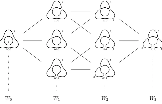
The crossings are all positive, so (n+, n−) = (3,0). From this diagram, we get the following cube of resolutions, where, as with computing the Jones polynomial, each vertex of the diagram will be a collection of disjoint circles. The circles are indexed by the smallest index of the arcs it contains:

000 010

001 100

101

011 110

111

W0 W1 W2 W3

1

2

1

1 2

1

2

1

3

3 2

[image:16.595.143.461.511.715.2]

1

(17)

where

W0=V1⊗V2

W1= (V1⊕V1⊕V1){1}

W2= ((V1⊗V2)⊕(V1⊗V2)⊕(V1⊗V3)){2}

W3= (V1⊗V2⊗V3){3}.

For each disjoint circle we assign a graded vector spaceVi=V =khv−, v+i, where deg(v±) =±1, so qdim(V) =q−1₊_q_{. Moreover, we index each}_V _{by the index of the circle that it corresponds}

to. At a given vertex of the cube of resolutions, we tensor the vector spaces corresponding to the circles in a smoothing diagram and apply a degree shift according to the number of 1 smoothings at the vertex. So at each vertex we haveV⊗k_{_r_} _{and qdim(}_V⊗k_{_r_{}) =}_qr₍_q−1₊_q₎k_{. We then}

take the direct sum down the columns to get the spacesCKh0(L)s=Ws.

Next we need to define differentials to make this into a complex. Each edge of the cube corresponds to a differential (of a subcomplex in homogeneousq-grading). We label the differentialsdαwhere

α∈ {0,1,∗}n_{, where there is a single}_{∗, and where}_n_{is the number of crossings in the link diagram.}

The ∗records which digit in the vertex’s index changes: for example, 0010 d0∗10

−−−→0110 since the second index in the two smoothings changes. We then sprinkle minus signs on the differentials to make the cube faces anticommute according to (−1)s_where_s_{is the number of 1’s before the}

star∗. For the mapsdα, we want them to have degree zero so that the graded Euler characteristic

returns the Jones polynomial. Since each column has a degree shift according to the number of 1 smoothings at the vertex, and this will increase by +1 from column to column, we must have the differentials to have degree−1. From vertex to vertex, either two circles will merge into one, or one circle will split into two circles. Since deg(v⊗w) = deg(v) + deg(w), Khovanov defines the differentials to be:

( → )

=m:V ⊗V →V v+⊗v+7→v+

v+⊗v−7→v−

v−⊗v+7→v−

v−⊗v−7→0 = ∆ :V →V ⊗V

v+7→v+⊗v−+v−⊗v+ v− 7→v−⊗v−,

and we setdαto be the identity on the circles that don’t participate. Since there is no order on the

circles in the diagram at each vertex, this forcesm and ∆ to be commutative and cocommutative, respectively. So, in particular, this forcesm(v+⊗v−) =m(v−⊗v+) andmand ∆ to be defined in

the above way up to scalars. By the indexing of vector spaces we can keep track of which circles are merged or split. So for the vector spaceVi⊗Vj, which has basis{v+i ⊗v

j

+, v+i ⊗v

j

−, v−i ⊗v

j

+, vi−⊗v

j

−}, we definemij :Vi⊗Vj→Vmin{i,j} and ∆ij :Vmin{i,j}→Vi⊗Vj. Thus, for example, in Figure 1.1,

d1∗1=−idV1⊗∆23, so

−d1∗1:V1⊗V2→V1⊗V2⊗V3

v1₊⊗v₊2 7→v1₊⊗v2₊⊗v₋3 +v1₊⊗v₋2 ⊗v₊3 v₊1 ⊗v2₋7→v1₊⊗v2₋⊗v3₋

(18)

An edge map will be of the following form: ordering the basis of V1⊗V2 to be (v+1 ⊗v+2, v+1 ⊗ v2

−, v−1 ⊗v2+, v1−⊗v−2) and the basis of V1⊗V2⊗V3to be (omitting⊗)

(v+1v 2 +v

3 +, v

1 +v

2 +v

3

−, v

1 +v

2

−v

3 +, v

1

−v

2 +v

3 +, v

1 +v

2

−v

3

−, v

1

−v

2 +v

3

−, v

1

−v

2

−v

3 +, v

1 −v 2 −v 3 −), we get the differential

d1∗1=

           

0 0 0 0

−1 0 0 0

0 0 0 0

0 −1 0 0 0 0 −1 0 0 0 −1 0

0 0 0 −1

            .

The differentials of our complexCKh(L)0_• will be the sum of the edge maps

d0=d∗00+d0∗0+d00∗

d1=d1∗0+d10∗+d∗10 d2=d∗01+d01∗+d0∗1 d3=d11∗+d1∗1+d∗11

We now have a complex CKh0(L) withrth spaceCKh(L)0_r. This is a complex because d2 _{= 0}

because the faces of the cube anticommuted.

Definition 1.10. We define the Khovanov complex to beCKh(L) =CKh0(L)[−n−]{n+−2n−}. In the case of the trefoil above, the Khovanov complex is thus

0→W0 d0

−→W1 d1

−→W2 d2

−→W3→0.

(Sincen− = 0,W0 is in homological height 0). Indeed, with these degree and height shifts, the graded Euler characteristic of this complex is, by construction, the unnormalised Jones polynomial:

χq(Kh(L)) = ˆJ(L).

Knowing the differentials, we can take homology. Sparing you the details, and letting our vector spaces be over the field_Q,

H0=Q{v−⊗v−, v+⊗v−−v−⊗v+} H1= 0

H2=Q

 

 



v−⊗v+

v−⊗v+ 

  



H3=Q{v+⊗v+⊗v+}

Thus, with grading shifts,

qdim(H0) =q+q3

qdim(H1) = 0 qdim(H2) =q5

qdim(H3) =q9

So the Poincar´e polynomial is

K(q, t) =X

k

(19)

Settingt=−1 returns the graded Euler characteristic, which is the unnormalised Jones polynomial:

K(q,−1) =q+q3+q5=q9= (q+q−1)(q2+q6−q8).

It turns out that this construction gives us a knot invariantKh(K) of a knot Kthat is stronger than the Jones polynomial. For example, ˆJ(¯51) = ˆJ(10132), but Kh(¯51)6=Kh(10132). To show

that it is a knot invariant, we should check that for two linksLand ˜Lthat differ by a Reidemeister move, thatKh(K)∼=Kh( ˜L) (the mapCKh(L)→CKh( ˜L) is a quasi-isomorphism of complexes). The interested reader can find this [Kho00] and [BN02].

1.2.3 A note on Functoriality

In addition to the quasi-isomorphismsCKh(L)→CKh( ˜L) between two link diagrams that differ by a Reidemeister move, we also have chain maps for ‘Morse moves’

∅ → , → ∅, → ,

called birth, death and fusion moves, respectively.

Given a link cobordism Σ, we can decompose it as a union of elementary cobordisms Σ1∪ · · · ∪Σk

given by the Morse and Reidemeister moves, and we would like to associate chain maps to each of these moves soCKh(Σ) :CKh(L)→CKh( ˜L) is the compositionCKh(Σ) =CKh(Σ1)◦ · · · ◦ CKh(Σk). Unfortunately, different ways of decomposing a cobordism gives different answers. For

example,

is just the identity, but however we pick our homotopy equivalences for Reidemeister moves, this composition is assigned −id. In fact, this is the best we can do: the description of Khovanov homology in this chapter is only functorial up to a minus sign. This was independently fixed by Clark, Walker and Morrison in [CMW09], Caprau in [Cap08] and Blanchet in [Bla10].

Thus, to summarise, Khovanov homology is a categorical link invariant. It sends objects in

C•=Kom(GVeck) and isotopies Σ between links LandL0 to isomorphisms in that category. The

Grothendieck groupK0(C•) isZ[q, q−1], and the image there is exactly the (unnormalised) Jones

polynomial.

L Kh(L) [Kh(L)] = ˆJ(L)

L0 Kh(L0)

Kh

Σ

K0

Kh(Σ)

Kh

(20)

0 0

This motivates the following chapter’s generalisation of Khovanov homology to tangles: if we start with a tangle, then its cube of resolutions will have at each vertex a complete smoothing that will be an element of HomTL, whereTLis the Temperley-Lieb category, which is a braided tensor

category defined by

• objects are the natural numbersN

• HomTL(n, m) is the freeZ[q, q−1]-module of planar diagrams withn‘input’ strands andm

‘output’ strands with no crossings

• composition is by stacking diagrams with common endpoints, replacing loops with q+q−1

• tensor product is by juxtaposing diagram horizontally.

In fact, the Hom space ofTL can be viewed as a category (soTL is a tensor 2-category) and we can look at the morphisms between the Hom spaces ofTL. This will be the content of Chapter 2. It turns out that Khovanov homology is associated to the braided tensor categoryRep(sl2(C))

(which is equivalent as a category to the idempotent completion ofTL) and there are more general Khovanov homology theories that are related to other Lie algebras, such assln(C). An introduction

(21)

CHAPTER 1. INTRODUCTION 1.3. TOPOLOGICAL QUANTUM FIELD THEORIES

1.3 Topological Quantum Field Theories

Before progressing onto the next chapter, the reader who is familiar with TQFTs (topological quantum field theories) may have noticed that we have applied a TQFT to the cube of resolutions. For those who are not familiar we will briefly describe this more general theory. This section is intentionally brief, since the the term TQFT is used throughout this paper but only its basic definition is used. For further introductory explanation of TQFTs, there are plenty of references such as [Koc04]. TQFTs have a functorial axiomatisation due to Atiyah on which we will base our discussion.

Definition 1.11. Ann-dimensional TQFT is a symmetric monoidal functor from (nCob,t,∅, τ) to (Vect_k,⊗,_k, σ). This is also called a linear representation ofnCob.

Here,nCob is the category whose objects are closed oriented (n−1)-manifolds and a morphism between two (n−1)-manifolds Σ and Σ0 is an oriented n-dimensional manifold M whose ‘in-boundary’ is Σ and whose ‘out-‘in-boundary’ is Σ0. This manifold (a cobordism) M is defined up to diffeomorphism relative its boundary. It does not need to be embedded in any ambient space, and can be considered as an abstract manifold.

Composition of morphisms is by gluing common boundaries (this is just topological gluing and the smooth structure is well-defined up to diffeomorphism). The identity cobordisms are cylinders. The symmetric monoidal structure ofnCobis as follows: the tensor product of two manifolds Σ and Σ0 is their disjoint union ΣF

Σ0 and the tensor unit zero is the empty manifold. The symmetry map τΣ,Σ0 : ΣFΣ0 → Σ0FΣ that switches the two factors is a diffeomorphism that provides

the symmetry structure. This extends to the disjoint union of cobordisms: given the cobordisms

M0: Σ0→Σ00 andM1: Σ1→Σ01 we can form the disjoint unionM0tM1: Σ0tΣ1→Σ00tΣ01.

In the casen= 2,2Cobis generated by disjoint sets of circles and the morphisms are obtained by composing 2 and tensoring the following basic building blocks:

There is an equivalence of categories between 2-dimensional TQFTs and commutative Frobenius algebras given by sending the TQFT to its value on the circle. A Frobenius algebra is an algebra which is simultaneously a coalgebra with certain compatibility condition between multiplication and comultiplication:

Definition 1.12. A Frobenius algebraAis a vector space with multiplication mapµ:A⊗A→A, unit η : k →A, a comultiplication map ∆ :A→ A⊗A, and counit : A →k, such that the

Frobenius relation holds:

(1⊗µ)◦(∆⊗1) = ∆◦µ= (µ⊗1)◦(1⊗∆).

(22)

(23)

Chapter 2

Bar-Natan’s Khovanov Homology

2.1 The Categorical Setting

Our goal is to apply different TQFTs to then-dimensional cube of resolutions we’ve just described. From this, we can obtain link invariants from any knot (or tangle) diagram by taking homology. Already, we have seen one such TQFT, the Khovanov TQFT, which for a link Lgives us a chain complexCKh(L). The following theory was developed by Bar-Natan [BN05] in order to extend Khovanov homology to tangles, giving us a ‘local’ Khovanov homology. Furthermore, we wish to develop our understanding of the category where the cube of resolutions is an object, so we can simplify the cube (its objects and morphisms)before we apply the TQFT, via Bar-Natan’s dotted theory. This will ultimately lead to savings in computational complexity.

As with Khovanov’s original homology theory, we want to think of such a cube obtained from a tangleT as a chain complexBN(T) in a certain graded category where we have direct sums. Each vertex of the cube of resolutions for a diagram has a complete smoothing. Thus, this category should have smoothings as objects and cobordisms for maps between these objects.

Definition 2.1. The category Cob3(∅) has the following data: it has smoothings (simple closed curves in the plane) as objects, and the morphisms are cobordisms between such smoothings regarded up to boundary preserving isotopies. We could also take a finite set of pointsB on a circle (such as the boundary∂T of a tangleT) and get the categoryCob3₍_B_{) which has as objects}

smoothings with boundaryB, and the morphisms again are cobordisms between such objects up to boundary preserving isotopy. In both cases, composition of morphisms is given by stacking cobordisms and then a rescaling.

For example if|B|= 2, a smoothing and a boundary preserving cobordism will look like

(24)

2.1. THE CATEGORICAL SETTING CHAPTER 2. B-N’S KHOVANOV HOMOLOGY

Remarks.

• There is a minor difference here with the category2Cobdefined earlier, where we now allow objects to be not necessarily closed (i.e. compact without boundary).

• The 3 in Cob3 refers to the fact that this category can be interpreted as a 3-category: there are 1-morphisms in Ngiven by addition, 2-morphisms between pairs of numbers given by

T L-diagrams, and then 3-morphisms that are surfaces betweenT Ldiagrams modulo isotopy. We will stack morphisms from top to bottom, as below, which hasg,f andf◦gfrom left to right:

You can think of the ‘input’ going into the bottom and the ‘output’ coming out of the top. Going back to our cube of resolutions, and having defined the objects and morphisms of our category, we also want therth chain space [[T]]r−n− _{of the complex [[}_T_{]] to be the ‘direct sum’ of the}

spaces (smoothings) at heightrin the cube, and sum the maps (cobordisms) to get a differential for [[T]]. To introduce direct sums into our category, we first make our category ‘pre-additive’.

Definition 2.2. Apre-additive categoryCis a category enriched in the monoidal category of abelian groups. So the morphisms between two objects form an abelian group, and the composition maps are bilinear in the sense that composition distributes over the group operation: f◦(g+h) =f◦g+f◦h. In particular, for anyA, B∈ob(C), there is a zero map 0∈HomC(A, B).

If the categoryC is not pre-additive, we can consider another category ˜Cwith the same objects and morphisms, but ˜C is pre-additive by takingZ-linear combinations of elements in HomC(A, B)

for any two objectsA andB, and by allowing composition to distribute_Z-linearly.

Example 2.3. The categoryAbof abelian groups is pre-additive. Without the commutativity,Grp

is not pre-additive since sums of group homomorphisms may not again be a group homomorphism, that is, it is not the case that we have the following for allf, g∈HomGrp(A, B), and all a, b∈A,

because we need commutativity for the third equality:

(f+g)(a+b) =f(a+b) +g(a+b) =f(a) +f(b) +g(a) +g(b) =f(a) +g(a) +f(b) +g(b) =f(a+b) +g(a+b).

Continuing in this vein,

Definition 2.4. Anadditive category is a pre-additive category with a zero object (a unique object that is both initial and terminal), and hence zero morphisms, and an additive category also has biproducts, denoted⊕.

Lastly, we describeabelian categories.

(25)

CHAPTER 2. B-N’S KHOVANOV HOMOLOGY 2.1. THE CATEGORICAL SETTING

This is the most general category in which we can work with homology, or rather, it is the most general setting where the Snake lemma holds. Examples include the categories Ab,R-Mod and

Vect_k.

Definition 2.6. IfC is a pre-additive category, then we can form a new additive category, called theadditive closure ofC,Mat(C), via the following:

• The objects ofMat(C) are formal direct sums⊕n

i=1Ai ofC.

• For two objectsA=⊕m

i=1Ai andA0=⊕nj=1A0j, a morphism between themF :A→A0 is an

n×mmatrixF = (Fij) where eachFij :Ai→A0j is a morphism inC.

• Morphisms in Mat(C) are added via matrix addition.

• Composition of morphisms is by matrix multiplication; i.e. (F◦G)ik:=P_jFij◦Gjk.

The categoryMat(C) is additive, and ifC was additive with biproduct⊕0_{, then no harm was done:}

X⊕Y ∼=X⊕0_Y_.

At this point, our cube of resolutions can be interpreted as a tower of morphisms between formal direct sums of smoothings. For example, for ann-crossing tangleT, we can interpret it as a length

ntower of morphisms between formal direct sums of smoothings

[[T]] = [[T]]−n− _→_[[_T_]]−n−+1_{→ · · · →}_[[_T_]]n+

.

In fact, these towers will be complexes, for which we provide the following definition.

Definition 2.7. LetC be a pre-additive category. ThenKom(C), ‘the category of complexes over C’, is the category with the following information:

• objects are complexes of finite length. . .−→Cn−1

dn−1

−−−→Cn dn

−→Cn+1−→. . . wheredndn−1=

0 for alln.

• morphisms between such complexes F : C → C0 are the set of maps {Fn} that give

commutative diagrams

· · · Cn−1 Cn Cn+1 · · ·

· · · Cn0−1 Cn0 Cn0+1 · · · Fn−1

dn−1

Fn

dn

Fn+1 d0_n₋₁ d0_n

where all arrows are morphisms in C. This is just the formal analogue of maps of chain complexes in homological algebra. CompositionF◦Gis defined as in ordinary homological algebra, (F◦G)n=Fn◦Gn.

We can consider these formal complexes up to homotopy, which works the same as the homological algebra case: let C be a category, andKom(C) its category of complexes. Then two morphisms

f, g: C• ⇒D• between complexes (C•, dC•) and (D•, dD•) are homotopic if there exist diagonal maps maps hn : Cn → Dn+1 so thatfn−gn =dDn+1hn+hn−1dCn, i.e. their difference is null

homotopic).

(26)

Now we are in a position to define the Khovanov complex [[T]] of an oriented tangle diagramT, this is going to be very reminiscent of Khovanov’s original construction, but now we think of the cube of resolutions as an object inKom(Mat(Cob3)).

Definition 2.8. Consider the diagram of a tangleT withn=n++n− crossings. As we did in Khovanov’s original construction, label each of the crossings from 1 ton. We will again construct the cube of resolutions, where at each vertex there is complete smoothing of the original tangle, described completely by a length n word of 0s and 1s. Two vertices are connected by an edge if and only the words at the vertices differ by one letter. We orient these edges by having the arrow directed towards the larger word (when the word is viewed as an integer). We then label the arrows by annletter word in{0,1,∗}where the∗is in the position where the words at the top and tail of the arrow differ:

0010−−−→0∗10 0110.

Lastly, to make each face of the cube anticommute, we sprinkle minus signs according to multiplying each differential with labelξ1ξ2. . . ξn by (−1)

P

i<jξj _where_ξ

j=∗(this is just to the power ofk,

where kis the number of 1s before the∗). Recall that in Kom(Mat(Cob3)) each differential is a matrix of cobordisms. The cobordism corresponding to an arrow is, in the cyclinder between the two smoothings that differ, the obvious saddle. Thekth column in the cube of resolutions (which is a direct sum of objects inMat(Cob3)) has homological heightk−n−.

Proposition 2.1. For any tangle diagramT, the chain[[T]]is a complex inKom(Mat(Cob3(∂T))). That is,d2= 0 for these chains.

Proof. Take any square in our cube of resolutions. We have to show that this square anticommutes. Firstly, as stated above, the cube of resolutions has minus signs sprinkled according to (−1)Pi<jξj_.

Thus in each square, the edges will have an odd number of minus signs. So we just need to show that morphisms (without minus signs) commute. Each vertex is labelled by a string of 0’s and 1’s, so as we traverse around the square, then, for example, theiandj index will switch toi+ 1 mod 2 andj+ 1 mod 2, respectively. To make it clear, the indices change +1 mod 2 as follows

{. . . i+ 1. . . j . . .}

{. . . i . . . j . . .} {. . . i+ 1. . . j+ 1. . .}

{. . . i . . . j+ 1. . .}

dj

di

dj di

The maps i→i+ 1 andj→j+ 1 are disjoint saddles, so the compositionsdjdi,didj are equal

since they are isotopic relative boundary (they are just a time reordering of saddles).

Remark 2.9. It is always possible to sprinkle minus signs on a cube so that each of the faces anticommute (so each face has an odd number of minus signs), and the space of choices in contractible. To see this, suppose you have a solid cube X = [0,1]n_{. We want a map}_σ_:_{{edges} → {±1}, i.e.}

an elementσin the 1-cocyles ofX with coefficients in{±1}=Z/2, soσ∈C1(X;Z/2), such that

for all facesA, Πedgeein∂Aσ(e) =−1. We also wantσsuch that,δ1σ=M inC2(X;Z/2), where

M(A) =−1 for all faces Aof X. Now, δ2M ∈C3(X;Z/2) and (δ2M)(X) = (−1)6= 1 (and 1

is our ‘zero’ in Z/2). So M is a 2-cocycle. But H2(X;Z/2) = 0 because X is contractible, so

kerδ = imδ, so there exists some σ such thatδ1_σ₌_M _{as desired. Moreover, suppose we had}

two sprinkling of signs σ and σ0_{. Then}_δ1₍_σ_·_σ0_{) = 0 which implies} _σ_·_σ0 _{is a 1-cocycle. But}

H1₍_X_;

Z/2) = 0, so there exists aτ ∈C0(X;Z/2) (soτ:{vertices} → ±1) such thatδ0τ =σ·σ0,

andτ(v)·τ(v0) =σ(e)σ0(e) whereeis an edge between verticesv andv0. Thereforeσ(e) =σ0(e) if and only if τ(v) = τ(v0). Define φ : [[T]] → [[T]]0 to be the map of complexes with different sprinkling of signs such that all faces anticommute, whereφis induced byτ(v)·id. Then φis an isomorphism of chain complexes.

(27)

so that [[T]] in Kom(Mat(Cob3_/_l)) is invariant up to homotopy of formal complexes. These local relations are described below, denotedS,T and 4T u respectively:

S

= 0

T

= 2

4Tu

+ = +

That is, when a cobordism contains a component isotopic to a 2-sphere, that cobordism is equal to zero. When a cobordism contains a component isotopic to a torus, it is equal to the same cobordism without the torus, but multiplied by 2. And the last relation says that you can change the cobordisms locally in the specified way.

We will write Kom/h(C) forKom(C) modulo homotopies. Moreover, we will use the shorthands

Kob(B) :=Kom(Mat(Cob3_/l(B))) andKob/h(B) :=Kom/h(Mat(Cob3/l(B))).

Theorem 2.10. The isomorphism class of [[T]] in Kob/h is an invariant of the tangle T. This

means that[[T]]does not depend on the ordering of the column vectors obtained from the cube of resolutions, and that it does not depend on the ordering of the crossings, and that it is invariant under the Reidemeister moves.

A proof of Theorem 2.10 can be found in [BN05].

This functor has excellent composition features by which we mean it is aplanar algebra.

Definition 2.11. Ad-input planar arc diagramD is an ‘output’ disk with the following data:

• dsmaller ‘input’ disks removed. The input disks are labelled 1 tod, each with a basepoint marked (this basepoint is often omitted from pictures).

• a collection of disjoint embedded arcs with endpoints intersecting the boundary of either the input or output disks transversely.

(28)

Definition 2.12. A collection of sets P(k) along with operations defined for each (oriented) unoriented planar arc diagram is an(oriented) unoriented planar algebra if

• the radial planar arc diagrams act as identities,

• associativity condition: ifDi is the result of pluggingD0 into theith hole of D (provided

this is possible), then as operationsDi=D◦(I× · · · ×D0× · · · ×I)

Note. In the categorical context, the axiom where the radial arc diagrams act as identities needs to be weakened, but can be safely ignored in this paper. For example, see [ETW17].

We usually consider the sets as topological objects, as in the above diagram, where we can place positive crossings into the operator that is the output disk. Let’s see how planar algebras come into play in this context. Firstly, consider the collection of all unoriented tangle diagrams in a based disk with kendpoints on the boundary, considered up to boundary preserving isotopies,

T0₍_k_{). Let}_T₍_k_{) be the quotient of}_T0₍_k_{) by the three Reidemeister moves. Then both}_T0₍_k_{) and} T(k) are planar algebras: letD be an output disk withki arcs intersecting theith input disk and

karcs intersecting the boundary of the output disk. Then we define the operator

D:T0(k1)×T0(k2)× · · · ×T0(kd)→T0(k)

by placing thedinput tangles into the holes ofD. The radial arc operators clearly act as identities, and the associativity condition also holds. We can define the planar algebraT(k) in the same way. More importantly for us, the collection ob(Cob3_/l) and Hom(Cob3_/l) are both planar algebras. The objects form a sub-planar algebra ofT(k). For the morphisms, consider a cylinder over the output diskD, D×[0,1]. This will havedcylindrical holes in it, connected by vertical curtains joining the top and bottom arcs inD× {0} andD× {1}. We can simply place cobordisms in the holes, defining an operationD: (Hom(Cob3_/l))d→Hom(Cob3_/l).

Now suppose we wish to place tangle complexes in the holes of a planar arc diagram, that is, put elements ofKob into planar arc diagrams. This will work like the tensor product of chain complexes, which we will define below for the unfamiliar reader.

Definition 2.13. Given two chain complexes (C•, dC) and (D•, dD), we can form the tensor product double complex, where the (p, q)th position of the lattice is (C⊗D)p,q=Cp⊗Dq. The

vertical maps aredv = (−1)p⊗dD and the horizontal maps are dh=dC⊗1. From the tensor

(29)

In Example 3.8 we show as an example how spectral sequences can be used to compute the homology of Tot(C⊗D) whereC andD are complexes of vector spaces.

For Kob(Bk) and Kob/h(Bk) (whereBk is a fixed placement ofk points on a based circle), we

define the operatorD, whereD is adinput planar arc diagram withki arc endpoints on theith

holes andkarc endpoints on the boundary of the disk, as follows: for a collection of complexes (Ci, di)∈Kob(ki),D(C1, . . . , Cd) is the complex (D, d) with components

Dj:=

M

j1+···+jd=j D(C_j1

1, . . . , C

d jd)

and differentials

d_D₍_C1

j1,...,C

d jd)

=

d

X

i=1

(−1)Pn<ijn_D₍_I

C1

j1

, . . . , di, . . . , ICd jd).

Properties of honest tensor products of chain complexes still hold in this case of tensor products of formal chain complexes. For example, morphismsf :Ci_→_Ci0_{induce morphisms}_D₍_{I, . . . , f, . . . I}_{) :}

D(C1_{, . . . C}i_{, . . . , C}d₎_→_D₍_C1_{, . . . C}i0_{, . . . , C}d_).

Proposition 2.2. The collection Kob(Bk)is a planar algebra. Moreover, the operatorsD acting

onKob(Bk)send homotopy equivalent complexes to homotopy equivalent complexes, so Kob/h(Bk)

is also a planar algebra.

Definition 2.14. A morphism Φ of planar algebras (P(k)) → (Q(k)) is a collection of maps Φ :P(k)→Q(k) such that for any operator DofP(k), Φ◦D=D◦(Φ×Φ× · · · ×Φ).

Definition 2.15. The Bar-Natan bracket [[−]] is an oriented planar algebra morphism [[−]] : (T(k))→Kob/h(Bk).

We are now due for an example which will hopefully make this all clear. Consider the oriented Hopf link, denoted 22

1, which can be viewed as the operatorD with input tangles that are a pair of

positive crossings:

22

1=D(X1, X2)

X

1

X

2

D X1=X2

Thus, [[22

1]] = [[D(X1, X2)]] =D([[X1]],[[X2]]) =tr([[X1]]⊗[[X2]]), where [[Xi]] = s

−

→ . Here, and thoughout this paper, the underline in the first space in the complex [[Xi]] denotes homological

(30)

Computing this tensor product,

tr([[X1]]⊗[[X2]]) = D( , )

D( , )

D( , ) ⊕

D(1, s)

D(s,1)

−D(1, s)

[[22

1]]0 [[221]]1 [[221]]2

⊕ =

.

−

Next we want to add some gradings to this category just we did in the original Khovanov theory. The rewards for this are great as it then allows us to read off the Jones polynomial as before.

Definition 2.16. Agraded category is a pre-additive categoryC with the following properties:

• for any two objectsC1, C2∈ob(C), the set of morphisms HomC(C1, C2) form a graded abelian group. Under composition, deg(f ◦g) = deg(f) + deg(g) for allf andg where this makes sense. Moreover, all identity maps have degree zero.

• there is an action by _Zthat ‘shifts degrees’: for an object C∈ob(C), and m∈Z, we can

define the same object but with a degree shiftC{m}. This does not change the morphisms between objects, i.e. HomC(C1{m1}, C2{m2}) = HomC(C1, C2), but changes the degrees of

the morphisms so that deg(f :C1{m1} →C2{m2}) = deg(f :C1→C2)−m1+m2.

Later, we will use the convention of recording the grading of an objectAwith gradingmbyqmA

rather thanA{m}, referred to as theq-grading.

So we can makeCob3andCob3_/l (and thusKobandKob/h) graded categories, where the grading is

(31)

Definition 2.17. LetC∈Hom(Cob3(B)) be a cobordism in a cylinder, with|B|vertical boundary components on the side of the cylinder. Then we define the degree of the morphism to be deg(C) :=χ(C)−1

2|B|.

This is also known as the relative Euler characteristic, which is computed by taking the Euler characteristic of the relative (simplicial) homology.

Example 2.18. The degree of a (upside down) pair of pants is−1 since it has Euler character-istic of−1 (it is homotopy equivalent to a twice punctured disk) and has no boundary components. The degree of a cap or cup is +1 since it is homotopy equivalent to a disk and also has no boundary components. The degree of a saddlesis−1 since it is homotopy equivalent to a disk (χ(s) = 1) and has four vertical boundary components so|B|= 4.

For our next definition, we will use ‘•’ to denote the zero object inKob/h.

Definition 2.19. LetT be a tangle diagram withn+positive crossings andn−negative crossings. DefineBN(T) to be the complex with each space in the complex

BNr(T) := [[T]]r{r+n+−n−}

and whose differentials are the same as the differentials of [[T]]:

[[T]] : • →[[T]]−n− _{→ · · · →}_[[_T_]]n+_{→ •}

BN(T) : • →[[T]]−n−_{_n

+−2n−} → · · · →[[T]]n+{2n+−n−} → •

SoBN(−) is just the complex [[T]] decorated with grading shifts. Thus, using the above definitions, we have

BN( ) =• →q −−−−→s q2 → •

BN( ) =• →q−2 −−−−→s q−1 → •

where sis the saddle cobordism.

Theorem 2.20. With the above gradings, BN(−)has the following properties: • All differentials forBN(T)for any tangleT have degree zero.

• The bracket BN(T)is a tangle invariant up to degree-zero homotopy equivalence. That is, if

T1 andT2 differ by a sequence of Reidemeister moves, then there is a degree-zero homotopy

equivalence F:BN(T1)→BN(T2).

• TheBN(−)induces a planar algebra morphism (T(k))→Kob(k), and all the planar algebra operations are of degree zero.

At this point, we have extended the original Khovanov homology of links to tangles. However, this category is clearly difficult to work with. To compare two tangles whose diagrams differ by a sequence of Reidemeister moves we need to construct an explicit homotopy equivalence between two complexes in Kob. To manage this, we will take a functor (a TQFT) from Kobinto some abelian category where we can take homology. Through this process we lose information but will be able to detect homotopy inequivalence much more easily.

(32)

2.2. TAKING HOMOLOGY OFBN(T) CHAPTER 2. B-N’S KHOVANOV HOMOLOGY

2.1.1 Adding dots

Next we will describe Bar-Natan’s dotted theory, which is how we will think of Khovanov homology and its variants from here on. We change our category Kob to its dotted version

Kob•=Kom(Mat(Cob•/l)), which will allow us to consider new homotopy equivalences.

This begins by extending the categoryCob3 to a category of dotted cobordismsCob3_•, where the objects are the same as Cob3, but morphisms can carry dots ‘•’ on them of degree−2. If 2 is invertible, dots are really a shorthand for

• = 1₂

The specified degree really makes sense since• is a genus 1 hole in our surface, and a punctured torus has relative Euler characteristic−2.

Dotted cobordisms are isotopic if the underlying cobordisms are isotopic and contain the same number of dots per component, and we consider morphisms up to boundary preserving isotopy. We then considerCob3_• up to local relationsCob3_•_/ldefined by

= 0 • = 1 •

•

= +

where the last relation is called the ‘neck cutting’ relation. Using these relations,

= 0

Notably, we also have the following computation,

Example 2.21.

= 1

8 +

= 1

8

So for example, if we additionally set the three holed torus to be zero, we have a sheet with two dots on it is also zero. As we will see below, this extra condition will return the original Khovanov homology.

2.2 Taking Homology of

BN

(

T

)

Up to now, we have extended Khovanov homology to the case of tangles by looking at a topological complex rather than an algebraic one. However, as a link/tangle invariant, it is difficult to work with, as it is difficult to construct explicit homotopy equivalences between complexes in Kob. Instead, we take a functor fromKobinto an abelian category, where if we take homology, we can find whether two complexes are not homotopy equivalent.

(33)

CHAPTER 2. B-N’S KHOVANOV HOMOLOGY 2.2. TAKING HOMOLOGY OFBN(T)

2.2.1 Choices of functor

F

We will outline two choices for the monoidal functor onCob3(∅) valued in the abelian category of graded_Z-modules_ZMod(we will also later work with _Q[α]-modules) that maps disjoint unions to tensor products. For this we define the functor on the generators of Cob3(∅). The objects of Cob3(∅) are generated by a single circle ○ (i.e. they are disjoint unions of circles) and the morphisms are generated by the cup , cap , pair of pants and upside down pair of pants .

Definition 2.22. Let V be the graded_Z-module freely generated by the two generators {v±} with grading deg(v±) = ±1. Let F be the TQFT defined viaF(○) = V, F( ) = : V → Z

(v− 7→1, v+7→0), F( ) =η:Z→V (17→v+) and most importantly, we have ‘multiplication’

F( ) =m:V ⊗V →V v+⊗v+7→v+

v+⊗v−7→v−

v−⊗v+7→v−

v−⊗v− 7→0.

and ‘comultiplication’

F( ) = ∆ :V →V ⊗V

v+7→v+⊗v−+v−⊗v+ v−7→v−⊗v−.

It can be checked that this indeed gives us a Frobenius algebra structure.

Proposition 2.3. The functor F is well-defined and the degree of the morphisms is preserved. Moreover F induces a functor Cob3/l(∅)→ZMod(so the local relations are preserved).

Proof. To see that F is well-defined, we have to see that it respects the relations between the generators ofCob3, or in other words the image of the functor has the structure of a Frobenius algebra. To see thatF is preserves the degrees of the morphisms, recall that a pair of pants (and an upside down pair of pants) has degree−1. This indeed is the case formand ∆, which lower the degrees by 1. The degrees deg(F( )) = 1 = deg(F( )) also checks out. To see thatF also induces a functor on the category modulo local relations, we note those relations:

S : 17−→v+7−→0,

and

T : 17−→v+7−−→v+⊗v−+v−⊗v+7−−→2v−7−→2.

The relation 4Tu also holds:

(34)

2.2. TAKING HOMOLOGY OFBN(T) CHAPTER 2. B-N’S KHOVANOV HOMOLOGY

because

(F( ))(1) = ∆1⊗1⊗1

=v−⊗v+⊗v+⊗v++v+⊗v−⊗v+⊗v+

:=v−++++v+−++

(F( ))(1) =v++−++v+++− (F( ))(1) =v+++−+v+−++

(F( ))(1) =v++−++v−+++.

Remark 2.23. It can be seen that for a linkL,H•(F(BN(L))) is equal to Khovanov’s categorifi-cation of the Jones polynomial. That is,CKh(L) =F(BN(L)).

So now we have a functor (TQFT) that defines Khovanov’s categorification of the Jones polynomial. Now we want to construct more functors, in particular the Lee TQFT. More generally, the Khovanov and Lee TQFTs are specialisations of the tautological functor:

Definition 2.24. LetB be a set of points on a circleS1 _{and let}_O _{be an object in}_Cob3

/l(B). So

Ois a smoothing with boundaryB. Thetautological functor FO :Cob3/l→ZModis defined on an

objectO0 _by_FO(O0_{) = Hom(O}_,_O0_{) and on a morphism}_F _:_O0 _{→ O}00 _by_FO₍_F_{) : Hom(O}_,_O0₎_→ Hom(O,O00_{) where}_FO(_F_{) (FO}_(O0_{)) =}_F_(FO(O0_)).

Example 2.25. TakeB=∅andO=∅. To make 2 invertible, tensor with _Z[1₂], and quotient out by all surfaces with genusg >1, so

F1(O) :=Z[

1

2]⊗ZHom(∅,O)/((g >1) = 0).

Taking two twice punctured disks (or equivalently, pairs of pants), and since 2 is invertible, the 4Tu relation becomes the neck cutting relation in Bar-Natan’s dotted theory.

+ = +

•

+ = 2 + 2

•

• +

= isotopy

(35)

CHAPTER 2. B-N’S KHOVANOV HOMOLOGY 2.2. TAKING HOMOLOGY OFBN(T)

Proposition 2.4. The functors F1(−)∼=F(BN(−)) =CKh(−)are isomorphic.

Proof. Firstly we will see how this works on objects:

Hom(∅,)∼=Zh , i ∼=Zhv−, v+i=V =CKh(),

where 7→ v− and 7→ v+ in the second isomorphism. Next, consider Hom(∅, ) ∼=

Zh , , , i. Then the pair of pants takes Hom(∅, )→Hom(∅,), by

7→

7→0

where the last map is because two dots are zero and neck cutting. With the above isomorphism on objects, we see this is exactly the Khovanov homologymmultiplication. A similar argument shows the isomorphism on the comultiplication, unit, and counit maps.

Example 2.26. (The Lee TQFT) Take the same as before, but instead of modding out by all surfaces of genus greater than 1, quotient out by the relation that all genus 3 surfaces are equal to 8:

F2(O) :=Z[1

2]⊗ZHom(∅,O)/( = 8).

Then as aZ[12]-module,F2(O) =F1(O) on objects, but ∆ andmare modified: m2:V ⊗V →V

v+⊗v+7→v+

v+⊗v−7→v−

v−⊗v+7→v−

v−⊗v−7→v+

and

∆2:V →V ⊗V

v+7→v+⊗v−+v−⊗v+

v−7→v−⊗v−+v+⊗v+.

To see how these maps are derived, take for example, ∈Hom(∅, ), then

m2(v−⊗v−) =F2( )(F2( )⊗ F2( )) =F2( ◦( )) =F2( ) =v+.

Remark 2.27. We could set the three-holed torus to be any invertible number (if we are in _Q, then anyα∈_Q∗_{) but we choose}_α_{= 8 so we can drop some constants. This was shown in Example} 2.21.

Remark 2.28. Here, we make the important remark that the gradings of the maps have been broken (they are no longer homogeneous) and thusF2 is not degree respecting. Thus, when we

apply the Lee TQFT to the complex inKob, the spaces in the chain complex are graded vector spaces (the same as the Khovanov TQFT spaces), but the induced differentials arenot graded. In fact, the differentials are filtered where the filtration is induced by the grading

· · · M

i>k+1 Vi⊂

M

i>k

Vi ⊂ · · ·

andd L

i>k+1Vi

⊂L

(36)

2.3. TOOLS AND COMPUTATION CHAPTER 2. B-N’S KHOVANOV HOMOLOGY

Thus we have two isomorphic ways to think of Khovanov homology and Lee homology:

• For a tangle T, Khovanov homology can be obtained via taking Hom(∅, BN(T)) and by quotienting out by all closed surfaces of genus greater than 1 (i.e. two dots on a surface is zero), and Lee homology can be obtained by taking Hom(∅, BN(T)) and by quotienting out by a genus 3 surface is equal to 8 (i.e. two dots can be pulled off a surface).

• This is the same as taking the Khovanov and Lee TQFTs ,CKh(−) and CKhLee_{(−), into}

the free modules_Zhv−, v+iwhich do the same thing to objects, but the multiplication and

comultiplication maps between the objects differ according to Definition 2.22 and Example 2.26.

We will denote the graded chain complex of vector spaces obtained by the Khovanov TQFT applied to a tangleT by CKh(T) and its homology to beKh(T). Similarly, we will denote the filtered chain complex of vector spaces obtained by the Lee TQFT byCKhLee₍_T_{) and the Lee homology}

byKhLee₍_T_{). We have for each space}_CKhLee₍_T₎

r=CKh(T)r, so the chain spaces are the same

but the differentials for the Khovanov and Lee complexes are graded and filtered respectively. A result by Lee in [Lee05] is that Lee homology is interestingly boring. To show this, she introduces a new basis{a, b}forV wherea=v−+v+andb=v−−v+. The multiplication and comultiplication maps become

m(a⊗a) = 2a

m(a⊗b) =m(b⊗a) = 0

m(b⊗b) =−2b

∆(a) =a⊗a

∆(b) =b⊗b

By using this basis, Lee proves thatKhLee₍_L_{) has rank 2}n_{, where}_n_{is the number of components}

ofL. Thus, working over_Q,KhLee₍_K₎_∼₌

Q⊕Qfor any knotK.

As we will show in Theorem 4.1, our focus on these two homology theories is because Khovanov homology can be naturally viewed as the second page of a spectral sequence (defined in the following chapter) that converges to Lee homology which is a surprisingly simple object.

2.3 Tools and Computation

There are a couple of tools from homological algebra which are useful in simplifying the chain complexes inKob. The idea is that when we make these simplifications before we take the tensor product of the chain complexes, we can reduce the number of computations.

Proposition 2.5. (Gaussian elimination) Suppose we have a segment of a chain complex in the additive categoryMat(C) of the form

· · · A B⊕C D⊕E F · · ·

  ξ β     φ δ γ   µ ν

whereφ is an isomorphism. Then the above segment of chain complex is isomorphic to the direct sum of complexes:

B D

· · · A C E F · · ·

φ

⊕ ⊕

β ₋_γφ−1_δ ν

(37)

CHAPTER 2. B-N’S KHOVANOV HOMOLOGY 2.3. TOOLS AND COMPUTATION

· · · A β C −γφ E F · · ·

−1_δ

ν

This is because the complexB−→φ D is contractible becauseφis an isomorphism.

Proof. Consider the change of basis matrices

T1=

1 φ−1_δ

0 1

T2=

1 0

−γφ−1 ₁

and denote M = φ δ γ .

Then we have the ‘row (and column) reduction’ ofM,

T2M T₁−1=

φ 0

0 −γφ−1_δ

as desired. Furthermore,

T1 ξ β =

ξ+φ−1_δβ β

(µ ν)T₂−1= (µ+νγφ−1 ν)

But since the original chain is a chain complex,d2_{= 0, so}

φ δ γ ξ β = 0

and thusφξ+δβ= 0, and

(µ ν)

φ δ

γ

= 0

and thusµφ+νγ= 0. This givesξ=−φ−1δβandµ=−νγφ−1, so

T1 ξ β = 0 β

, and (µ ν)T2= (0 ν).

Proposition 2.6. (Delooping) If an object S in Cob3_•_/l contains a closed loop , then it is isomorphic in Mat(Cob3_•/l) to the direct sum of copies S0{+1} and S0{−1} of S in which is

removed, one taken with a degree shift of +1 and one with a degree shift of −1. Symbolically, ∼=∅{+1} ⊕ ∅{−1}.

Recall that if an objectOhas a gradingO{m}, we will write the gradings using aqinstead, so O{m}will be recorded asqm_O.

Proof. The isomorphisms are as follows:

∅{−1}

∅{+1}

⊕

•

(38)

2.3. TOOLS AND COMPUTATION CHAPTER 2. B-N’S KHOVANOV HOMOLOGY

To verify this is an isomorphism, this uses all of the relations in Cob3_•/l. The map → is an

isomorphism since

→ = ( )

= + = = 1

where the third equality is the neck cutting relation. To see f :∅{−1} ⊕ ∅{+1} → ∅{−1} ⊕ ∅{+1} is an isomorphism,

f =

( ) =

! =

1 0 0 1

.

Example 2.29. Let’s see these tools in action. In our previous example for finding the Khovanov complex for the Hopf link, we could have simplified the complex using these tools. We will now find the Khovanov complex for the right-handed trefoil 31. Importantly, we will also keep track of

the gradings in this example.

Consider the oriented planar arc diagram from Definition 2.11:

T1

T2

T3

and takeT1=T2=T3= so D(T1, T2, T3) = 31. Then

BN(31) =BN(D(T1, T2, T3)) =D(BN(T1), BN(T2), BN(T3)).

To compute this, we will build this up step by step using the properties of planar algebras, simplifying as we go. Firstly, the concatenated positive crossings is computed by taking the tensor product of the complex BN( ). Then to obtain the knot, we then take the trace: we join the top right strand to the bottom right strand, and then join the top left to the bottom left. For

BN( )⊗3_{, we have the simplified expressions}

BN( ) =q −→s q2

BN( )⊗2'q2 →−s q3 −−−−−−− →q5

BN( )⊗3'q3 −→s q4 −−−−−−− →q6 −−−−−−+ →q8 .

More generally, we have for a two strand tangle withntwists:

(39)

CHAPTER 2. B-N’S KHOVANOV HOMOLOGY 2.3. TOOLS AND COMPUTATION

where a= − andσ= + alternate (for example, see [Tho17]). Joining the top right to the bottom right, take

BN( )⊗3

=q3 q4 q6 2 q8

zero

∼ =

q2

⊕

q4

q4 zero _q6 2 _q8

'q2 _• _q6 2 _q8

where the isomorphism is by delooping and the'(homotopy equivalence) is by Gaussian elimination. The above tangle is isotopic to the cut trefoil which we denote c(31). Thus

c(31)'q2 → • →q6 2

−−−→q8

And then lastly, we join the top left to the bottom left:

BN( )⊗3

=q2 _• _q6 2 _q8

∼

=q∅ ⊕q3∅ •

q5∅

q7_∅

q7∅

q9_∅

⊕ ⊕

'q∅ ⊕q3∅ • q5∅ 2 q9∅

Again, the isomorphism is by delooping and the homotopy equivalence is by Gaussian elimination. Since two dots on a cobordism is zero in Khovanov homology, we have the following if we work over_Q:

CKh(31) = HomQ(∅, BN(31))/( = 0)'qQ⊕q3Q→ • →q5Q−−→zero q9Q,

and Poincar´e polynomial

K(q, t) =q+q3+t2q5+t3q9.

In Lee homology, = α , where α∈ Q∗, so the portion of chain complex q5Q→ q9Qis

contractible, and thus

CKhLee(31) = HomQ(∅, BN(31))/( =α)'qQ⊕q3Q.

(40)

Understanding the Lee Spectral Sequence