SPH modelling of depth-limited turbulent open channel flows over rough boundaries

SPH modelling of depth-limited turbulent open channel

fl

ows over

rough boundaries

Ehsan Kazemi, Andrew Nichols, Simon Tait and Songdong Shao*

Department of Civil and Structural Engineering, The University of Sheffield, Mappin Street, Sheffield S1 3JD, UK

SUMMARY

A numerical model based on the smoothed particle hydrodynamics method is developed to simulate depth-limited turbulent open channel flows over hydraulically rough beds. The 2D Lagrangian form of the Navier–Stokes equations is solved, in which a drag-based formulation is used based on an effective roughness zone near the bed to account for the roughness effect of bed spheres and an improved sub-particle-scale model is applied to account for the effect of turbulence. The sub-particle-scale model is constructed based on the mixing-length assumption rather than the standard Smagorinsky approach to com-pute the eddy-viscosity. A robust in/out-flow boundary technique is also proposed to achieve stable uniform flow conditions at the inlet and outlet boundaries where theflow characteristics are unknown. The model is applied to simulate uniform open channelflows over a rough bed composed of regular spheres and validated by experimental velocity data. To investigate the influence of the bed roughness on differentflow condi-tions, data from 12 experimental tests with different bed slopes and uniform water depths are simulated, and a good agreement has been observed between the model and experimental results of the streamwise ve-locity and turbulent shear stress. This shows that both the roughness effect andflow turbulence should be addressed in order to simulate the correct mechanisms of turbulentflow over a rough bed boundary and that the presented smoothed particle hydrodynamics model accomplishes this successfully. © 2016 The Authors International Journal for Numerical Methods in Fluids Published by John Wiley & Sons Ltd

Received 22 October 2015; Revised 24 March 2016; Accepted 23 April 2016

KEY WORDS:SPH; turbulence; open channelflow; rough bed; drag force; inflow/outflow boundaries

1. INTRODUCTION

Because all natural river flows around the world are turbulent and the channel beds are often composed of large-scale, potentially mobile, rough elements such as sand and gravel particles, the study of turbulent open channelflows over rough beds is of significant engineering interest. This interest has motivated researchers to carry out various studies to explore theflow behaviour near the solid–fluid interface in laboratory experiments or to simulate the effect of bed roughness on theflow by numerical methods. The solution of fundamental hydrodynamic equations has become a popular numerical technique in modelling turbulentflows because it can provide time-dependent details of the flow characteristics such as velocities, pressures and transport properties. In turbulence modelling of open channel flows, the Reynolds-averaged Navier–Stokes (N-S) equations or space-filtered large eddy simulation (LES) equations have been widely used, where the large eddies are resolved and the small ones are modelled by an appropriate model, usually the eddy-viscosity model. The eddy-viscosity model relates the turbulent shear stress to the local strain rate through an eddy-viscosityνtbased on the Boussinesq approximation. A simple, economical and practical

*Correspondence to: Songdong Shao, Department of Civil and Structural Engineering, The University of Sheffield, Mappin Street, Sheffield S1 3JD, UK.

†_{E-mail: s.shao@sheffield.ac.uk}

approach to evaluateνtis using a mixing-length model that is known as the zero-equation model. In

this approach, the eddy-viscosity is related to the mean strain rate from Prandtl’s theory by using a turbulence characteristic lengthlmas follows:

νt¼lm2

dU dz

; (1)

where Uis the mean streamwise velocity and lmis the mixing length. Although the mixing-length

model is easy to use, it lacks the universality and is not applicable to complicated flows (e.g. 3D non-uniform flows with disturbed free surface) where the distribution of turbulence length scale lm

is not known. A well-known turbulence model that is commonly used for such complicatedflows is the two-equationk–εmodel where a wall function technique is usually used to estimate theflow in the shear boundary layer. Although this model has the advantage of including the effect offlow history and transport on the turbulence, it meets difficulties in treating rough wall boundaries because the near-bed logarithmic law does not hold anymore when large roughness elements exist. This has also been investigated by Nikoraet al.[1], who showed that in the interfacial sub-layer, which is theflow region between the roughness crest and trough, the velocity profile can be either constant, exponential or linear based on the flow conditions, relative submergence and roughness geometry. Another deficiency of the wall function approach has been addressed by Nicholas [2], in that the shear stress could not be accurately reproduced by a wall function approach because of the mesh resolution problems in the region near the rough bed. On the other hand, the LES modelling approach is based on the spatially averaged equations where usually a sub-grid-scale model is used to relate the turbulent eddy-viscosity with the localflow strain rate by using the Smagorinsky model [3].

Different approaches have been adopted to account for the roughness effect in numerical modelling of turbulent flow over rough walls. Some have been developed based on modifying the turbulence model near the rough boundary; while in some others, separate models have been used, for example, the roughness effect being formulated on the basis of a drag force equation. Van Driest [4] proposed a modification to his mixing-length formula originally derived for hydraulically smooth walls. Based on this modification, the shear stress was increased near the wall because of the existence of the roughness elements. Rotta [5] proposed a different modification to the van Driest formula by introducing a shift in the wall coordinate in order to increase the shear stress near the wall to take the roughness effect into account. Despite their simplicity, these models have provided a physical description offlow pattern near the wall and have been applied in several studies for calculation of boundary layers on rough walls, for example, in Cebeci and Chang [6]. However, their modified model is not suitable in cases where the wall is composed of large-scale discrete rough elements such as in gravel bed rivers. Hence, other researchers have explicitly modelled the roughness effect by using a drag-based model in which a sink term of the form drag is added to the momentum equations to address the form drag effect on the near-wall flow. Christoph and Pletcher [7] and Tayloret al.[8] used such models to simulate the roughness effect together with a mixing-length model to account for the turbulence. Wiberg and Smith [9] divided the total shear stress into a fluid shear component and a form-induced component and used a mixing-length model for the former and a drag force equation for the latter to calculate the velocity distributions in a steep stream over coarse gravel beds. Besides these, Cuiet al.[10], Carneyet al.

[11] and Zeng and Li [12] are some other examples of studies in which the drag concept has been applied to model the effect of wall roughness on theflow. Among them, Zeng and Li [12] used a wall function approach to treat the shear boundary for small-scale rough bed elements and a drag force model for large-scale rough beds when the wall function approach was unable to reproduce the correct velocity distributions.

Gotohet al.[13] and Shao and Gotoh [14, 15] should be mentioned. Recently, several other studies have been carried out focussing on the enhancement of the accuracy of particle methods in fluid

flows, for example, Khayyer and Gotoh [16], Lindet al.[17] and Gotohet al.[18]. Besides, further studies have also been performed to improve the modelling of the effect of wall and free surface boundary conditions, for example, Ferrandet al.[19], Leroyet al.[20] and Tsurutaet al.[21].

However, very few cases have involved open channelflows, although some pioneering works in thisfield have been reported such as by Federicoet al. [22] and Fu and Jin [23]. Because of this, turbulence and rough bed issues have not been effectively solved for the type of flows found in shallow rivers with a rough boundary. For turbulence models in SPH, the earliest and most comprehensive work could be attributed to Gotohet al.[24] and Violeau and Issa [25]. The former proposed a novel eddy-viscosity-based sub-particle-scale (SPS) turbulence model for a turbulent jet based on the moving particle semi-implicit (MPS) method, in which the turbulent quantities were validated but the model applications were mainly based on the smooth wall. The latter developed two Reynolds-averaged N–S turbulence models and also applied a LES approach to simulate more complex turbulent free-surfaceflows.

As for the shear boundary treatment, Violeau and Issa [25] used a wall function approach to impose the logarithmic velocity distributions near the wall. Besides, Lopez et al.[26] developed an SPH model with variable artificial viscosity to simulate hydraulic jumps, and they applied a Lennard–Jones repulsive force on the bed particles to produce a ‘numerical’ resistance on the near-wallflow. Sahebariet al.[27] and Fu and Jin [23] used the SPS model with Smagorinsky con-stantCs= 0.15 in their MPS simulations of open channelflows. Sahebariet al.[27] did not treat the

bed roughness effect, while Fu and Jin [23] adjusted the velocity of dummy particles near the bed boundary to take the roughness effect into account. In this way, different types of bed conditions, including smooth, intermediately rough and fully rough beds, have been studied. Chern and Syamsuri [28] also used the SPS turbulence modelling approach but withCs= 0.12 and simulated

hydraulic jumps over corrugated beds by using SPH. They treated the wall boundaries of smooth, triangular, trapezoidal and sinusoidal shapes by using lines of the particles and applied a repulsive force similar to that of Lopezet al.[26]. De Padovaet al.[29] employed an eddy-viscosity model based on the mixing-length concept forflow turbulence to simulate hydraulic jumps in a large chan-nel by SPH. Nevertheless, no bed boundary treatment was included in their model. Araiet al.[30] applied a wall function to estimate the near-wall velocity in their MPS model with a Smagorinsky-based eddy-viscosity model for turbulence in a LES of turbulent channelflows. A more physically sound rough bed modelling approach was initiated by Gotoh and Sakai [31] for a breaking wave inside a porous medium. They pointed out that a drag force equation could be the most appropriate way to address the bed roughness. Khayyer and Gotoh [32, 33] developed a more mature drag force model to address the wall friction effect for a dam breakflow over a wet bed. Besides, it is also worth mentioning that recently, quite a few influential works have been carried out in open channel

flows by using the concept of shallow water SPH [34–36].

In two recent studies, Mayrhoferet al.[37, 38] effectively investigated the turbulence modelling of wall-boundedflows using SPH. Mayrhoferet al.[38] introduced an additional volume diffusion term into the continuity equation in order to treat the noises that arise as a result of the SPH discretization. They used an eddy-viscosity model with a mixing-length approach to estimate the additional diffusion term. More recently, Mayrhoferet al.[37] applied the SPH method in a direct numerical simulation (DNS) as well as LES of 3D wall-bounded turbulent channel flows and revealed interestingfindings. Theyfirstly performed a quasi-DNS of a 3D channelflow based on SPH and achieved good agreement with the reference data except for some near-wall oscillations. Then they carried out a LES of a channelflow with frictionRenumber (Re_τ) of 1000 using SPH with the unified semi-analytical wall boundary condition and an eddy-viscosity model with the Smagorinsky constant Cs= 0.065 for the unresolved part of the turbulence. In contrast to the

In grid-based LES, a variable resolution is usually adopted so as to use a muchfiner mesh near the wall boundary in order to resolve the near-wall flow scales, while in SPH, a non-variable homogenous discretization has to be used. Hence, a wall function is usually applied, such as in the studies of Violeau and Issa [25], Araiet al.[30] and Mayrhoferet al.[37], to account for the wall effect.

In a most recent study in this area, Kazemiet al.[39] completed a comprehensive review on the numerical modelling of turbulent open channelflows over rough bed boundaries. They focused on the procedures of turbulence modelling and rough bed boundary treatments and reviewed mesh-free particle models that have been developed for these purposes. They remarked the deficiency of the eddy-viscosity models with the Smagorinsky constant in treating the turbulence effect in SPH sim-ulation of highly turbulent channelflows over rough boundaries, and also the insufficiency of the wall functions in treating the rough wall boundaries, which occurs because the near-wall velocity profile is not always logarithmic when the boundary consists of large roughness elements. Accord-ingly, the SPH method was recommended to be coupled with a mixing-length model for turbulence and a drag force equation model to treat the shear boundary near beds with large-scale roughness. In the present study, the proposed model is further developed and used to investigate the effects of bed roughness in different regimes of turbulentflow over rough bed boundaries. In summary, we will use the fundamental eddy-viscosity-based SPS model proposed by Gotoh et al.[24] but adopt a mixing-length approach to realistically calculate the eddy-viscosity to improve the turbulence model performance in open channelflows. As for the drag force model, we will improve it by in-cluding a shape function in the drag force equation to account for the shape of bed roughness ele-ments so as to more realistically evaluate the bed surface geometrical conditions. Also, an efficient inflow/outflow boundary treatment is used to generate an accurate and stable uniformflow along the channel. In model applications, the depth-limitedflows with different regimes but with the same bed roughness are simulated, and the velocity and shear stress profiles are validated by experimental data for 2D rough bed turbulentflow. Following Chenget al. [40], we consider the depth-limited condition as when the ratio of the bed roughness size to the water depth is significant. As far as we know, no documented SPH works have reported the quantification of such flow information for turbulent open channelflows over rough beds for conditions similar to those found in gravel bed rivers.

2. NUMERICAL MODELLING SCHEME

2.1. Governing equations

The governing equations are the two-dimensional continuity and momentum equations in the Lagrangian framework. An additional term to represent the form drag of the bed particles is included. This term as well as the turbulent shear term is not needed in a DNS. Thefinal equation reads

Dρ

Dt ¼ ρ∇u; (2)

Du

Dt ¼

1

ρ∇Pþgþν0∇2uþ

1

ρ∇τtþ

1

ρτd; (3)

wheret is the time, ρ is the fluid density, u is the velocity,P is the pressure, gis the gravitational acceleration,ν0is the kinematic viscosity coefficient,τtis the turbulence stress tensor andτdis the form

drag-induced shear stress from the rough bed.

To model the turbulence stress, an SPS model based on the eddy-viscosity assumption [24] is used as follows:

τij

ρ ¼2νtSij

2

whereiandjdenote the 2D coordinate components,τijis the component of shear stress tensorτt,Sijis

the component of strain tensorS calculated by Eq. (5),νtis the turbulence eddy-viscosity,k is the

turbulence kinetic energy calculated by Eq. (6) andδijis the Kronecker delta function.

Sij¼

1 2

∂ui ∂xjþ

∂uj ∂xi

; (5)

k¼νt ∂

ui ∂xiþ

∂uj ∂xj

; (6)

where x and u are the position and velocity components, respectively. In SPH, the turbulence eddy-viscosityνtis usually estimated by the Smagorinsky model [3], following the initiatives of Gotoh

et al.[24], as follows:

νt ¼ðCsΔÞ

2_S

j j; (7)

whereCsis the Smagorinsky constant, usually taken to be between 0.1 and 0.15,Δis the characteristic

length scale of eddies (filter width), which is taken as the particle spacing, and j j ¼S pffiffiffiffiffiffiffiffiffiffiffiffiS:ST is the local strain rate. It should be noted that the turbulence has a three-dimensional nature, and in particular for the spatially averaged LES-based modelling and consideration of SPS turbulence closure, the three-dimensional characteristics of turbulence should play an important role. However, in the present simulations of open channel uniformflow, theflow is dominated by the streamwise shear stress and vertical 2D momentum exchange, while the lateral influence is quite small so as to be reasonably neglected in this study.

Equation (7) has been used with SPH in several coastal hydrodynamic applications, and the accuracy has proved to be satisfactory. However, its applicability in open channel flows with SPH has been under-reported. In our previous computational experience [39], the Smagorinsky-based SPS model withCs= 0.15 was not able to reproduce the correct shear mechanism in a uniform

open channelflow over a rough wall. Also, in the study of Mayrhoferet al.[37], using an eddy-viscosity model with a Smagorinsky constantCs= 0.065 in the SPH-LES showed very poor results

with an overestimation in the streamwise velocity. They pointed out that the failure was related to the pressure–velocity interactions of vortices and concluded that this problem is inherent in the stan-dard SPH discretization.

We also carried out some simulations with the Smagorinsky constantCs= 0.15 to investigate this

issue. The results are presented in Section 3.4, which shows the failure of the SPH using the standard Smagorinsky eddy-viscosity model for turbulence. The failure is attributed to the deficiency of the standard Smagorinsky model in dealing with the cases in which sharp changes take place in theflow velocity, like the one studied in present work. Further discussions on this issue will be provided in Section 3.4. An alternative approach adopted here is then to explore the concept of a standard mixing-length model to estimate the turbulent eddy-viscosity in present SPH scheme in or-der to recover the part of the turbulence that cannot be captured by the standard Smagorinsky model with aCsbeing around 0.15. Accordingly, the eddy-viscosity is formulated as follows:

νt¼lm2j jS; (8)

where the mixing lengthlmis calculated by the Nezu and Rodi [41] empirical formula as follows, which

has been derived on the basis of physical measurements.

lm

H¼k

ffiffiffiffiffiffiffiffiffiffiffi

1ξ

p 1

ξþπΠsinð Þπ ξ

whereHis the water depth,kis the von-Karman constant andξ=z/His defined in whichzis the vertical coordinate, andΠis the Coles parameter.Πhas been introduced to describe the deviation from the log law in the outer region. This parameter comes from an empirical wake function added to the velocity log law by Coles [42]. Coleman [43] has also expressed that the deviation in the outer layer from the log law should not be accounted for by adjusting the von-Karman constantkand/or the integration constant (Br

in Eq. (21)) but rather by adding a wake function to the log law equation (Eq. (21)). However, in the present study, a value of 0.41 is adopted for k, and Πis assumed to be 0 so that the following Eq. (10) is used to estimate the mixing length that is a simplified form of Eq. (9). This formula has also been used in the studies of Violeau and Issa [25] in modelling the turbulent open channelflows by the SPH method.

lm¼kz

ffiffiffiffiffiffiffiffiffiffiffiffi

1-z=H

p

: (10)

Consideringxand zas the streamwise and vertical coordinates in a strongly 2D uniform open channel flow, and u and w as the streamwise and vertical velocity components, respectively, Eq. (8) would be equivalent to Prandtl’s theory (Eq. (1)), as the local strain rate |S| is approximately equivalent to∂u/∂zbecause of the other velocity gradients such as∂u/∂x,∂w/∂xand∂w/∂zbeing significantly smaller.

To account for the effect of bottom roughness, the form drag-induced shear termτd/ρshould be added to the momentum equation (3), because the macroscopic N-S equations are considered rather than a high spatial resolution (DNS) is solved for the refined flow details within the roughness region, which could use considerable CPU resources.τdwill be calculated by following Eq. (11), whereFdis the drag force exerted on thefluid particle from the rough bed, which is assumed to

be equal to and in the opposite direction of the force from the fluid particle acting on the bed.

A_τis the bed-parallel, planar area affected by thefluid particle. Furthermore, the drag forceFdwill

be calculated by Eq. (12), whereCdis the drag coefficient, Adis the planar cross-sectional area

and Wdis a non-dimensional shape function accounting for the geometry of the bed roughness.

The quantifications of relevant drag parameters will be detailed in Section 2.3.

τd ¼Fd

A_τ; (11)

Fd¼

1

2CdWdρAdu uj j: (12)

2.2. Discretization of equations by smoothed particle hydrodynamics

The numerical scheme based on the weakly compressible SPH (WCSPH) method is used to discretize the governing equations. SPH is a Lagrangian particle method that was developed by Gingold and Monaghan [44] initially for astrophysical problems. Since then it has been widely used for simulating fluid flows. In the SPH approximation, any variable, for example

A(r), can be estimated by the following integral interpolant equation as:

Að Þ ¼r

∫

ΩAð Þr′ Wðjrr′j;hÞdr′; (13)

whereΩ is the volume of the integral,ris the particle position,r′denotes the particle coordinate,his the smoothing length andW(|rr′|,h) is the weighting or kernel function. The aforementioned equa-tion can be expressed in the following discretized form to calculate A(r) at the position of particlea:

Að Þ ¼ra ∑ b

mb

Að Þrb ρb

where aandbare the reference particle and its neighbour and mbandρbare the mass and density of

neighbouring particleb, respectively. The derivative ofA(r) in thexjdirection can be approximated by

the following:

∂Að Þra ∂xj ¼∑b

mb

Að Þrb ρb

∂Wðjrarbj;hÞ ∂xj :

(15)

By using the aforementioned SPH formulations, the governing equations (Eqs (2) and (3)) are discretized as follows for the computations of density and velocity of the particles:

Dρ_a Dt ¼ρa∑_b

mb ρb

uab∇aWab; (16)

Dua

Dt ¼ ∑b

mb

Pa ρa2

þPb ρb2

∇aWabþgþ∑ b

mb

4ν0

ρaþρb

ð Þ

rab∇aWab rab j j2

þη2uab

þ∑

b

mb τa ρa2

þ_ρτb b2

∇aWabþ

1

ρa τd

ð Þa; (17)

where uab=uaub and rab=rarb are defined, ∇aWab is the gradient of the kernel function

between particles aandbwith respect to the position of particle aandη is a small number used to prevent singularity. In the present WCSPH model, the following Eq. (18) is used to link the continuity equation with the momentum equation to compute the fluid pressure from the change in particle density in an explicit way as follows:

P¼c02ðρρ0Þ; (18)

whereρ0is the reference density andc0is the speed of sound. In a WCSPH numerical scheme, it

is assumed that the flow is slightly compressible so the speed of sound should be chosen to be around 10 times of the bulk flow velocity to ensure the fluid compressibility being less than 1%. Finally, ρ0 and c0 are respectively taken as 1000 kg/m3 (water density) and 16 m/s as a

common practice in the computations. Since the WCSPH is known to result in considerable nu-merical noise in the pressure field, a special treatment (density filtering, delta-SPH terms, etc.) could be undertaken to improve the performance. Therefore, the present WCSPH simulations have been performed using a Shepard density filter to minimize the pressure noise at every 30 computational time steps. The solution method using a predictor–corrector scheme [45] is implemented to solve the governing equations and update the density, velocity and position of the particles. The selection of the computational time step follows the Courant–Friedrichs–Lewy condition.

2.3. Boundary conditions

2.3.1. Treatment of inflow/outflow boundary. Recently, some pioneering works have been carried out on the treatment of inflow/outflow boundary conditions in SPH, for example, Federico et al.

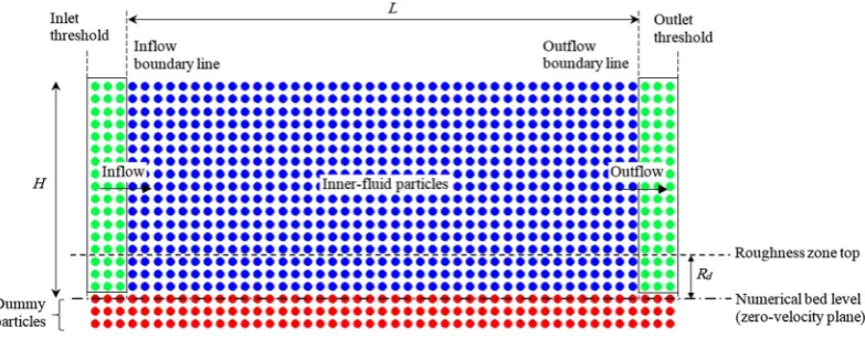
[22], Aristodemoet al. [46] and Tan et al. [47]. In present study, a similar technique has been adopted but with the difference in that the inflow particle velocities are linked with those of the innerfluid particles, so that theflows are evolved naturally without any prescription of the inflow velocity. For the inflow and outflow boundaries, several layers of particles are located beyond the boundary line but within the threshold line to cover the truncated kernel area of the inner-fluid par-ticles near the boundary (Figure 1). The governing equations are not solved for these parpar-ticles, but they move according to theflow conditions inside the inner-fluid domain. In this way, the velocity and pressure of inflow/outflow particles are evolved through calculations rather than being allocated the prescribed values. The proposed technique is suitable for cases where the inflow and/or outflow conditions are not known and need to be determined through the simulations. One example is the gravity-drivenflow over a sloping channel bed that is considered in the present study. To generate an open channel uniformflow, the appropriateflow conditions need to be achieved at the inflow boundary, that is, the gradients of the velocity and pressure in the streamwise direction xshould be 0 at the boundary line, represented by the following:

∂u

∂x¼0;

∂P

∂x¼0:

(19)

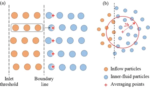
To satisfy these conditions in an SPH computation, the properties of the inflow particles (e.g. ve-locity and density) are set equal to those of the inner-fluid particles near the inflow boundary line. To do so, an averaging point isfirst defined for each inflow particle at the same elevation but inside the inner-fluid region, with a distance ofdp/2 from the boundary line as shown in Figure 2(a), where

dpis the SPH particle size. Then the velocity and density of the inner-fluid particles are averaged

over a kernel area onto these points and set as the velocity and density of the corresponding inflow particles (Figure 2(b)). Therefore, the gradient of velocity as well as the density is 0 at the boundary. Because the pressure is calculated by using Eq. (18), the zero pressure gradient is also satisfied, and thus, theflow uniformity is achieved. When an inflow particle crosses the boundary line and enters the inner-fluid region, it becomes an inner-fluid particle, and the governing equations are solved for it in the next time step. Meanwhile, an additional inflow particle is generated with the same prop-erties at the inlet threshold line for the same elevation (Figure 2(a)). In this way, the inflow region bounded by the inlet threshold line and the inner-fluid area acts like a particle generator to reach a uniformflow condition at the boundary. For consistency, the same kernel function and smoothing length of the inner-fluid SPH calculations are used for the averaging process in Figure 2(b). The novelty of the proposed inflow boundary treatment over that of existing approaches is that theflow is naturally evolved through the numerical simulations without being given a prescribed inflow

velocity, so the model can be applied to a much wider range of hydraulic applications in which the inflow information is unknown.

At the outflow boundary, the uniformflow condition should also be satisfied to keep the unifor-mity of theflow through the simulation domain. The same technique used at the inflow boundary can be used for the outflow one. However, a slightly different treatment is adopted at the outlet to reduce the computational time. When an inner-fluid particle goes across the outflow boundary line, it becomes an outflow particle, and the governing equations are not solved on the particle any-more, but its properties are kept unchanged when it moves through the outflow region. This treat-ment is similar to that used by Federicoet al.[22], in which the properties of outflow particles are frozen. Finally, the particles are removed from the computational domain when they pass through the outlet threshold line (Figure 1).

To check whether the inflow/outflow boundary condition satisfies the volume conservation or not, we simply calculated the volumeflows inside the computational domain at the inlet as well as thatflows out of the domain at the outlet boundary at every second of the simulation for several test cases, and we found out the maximum difference between the inlet and outlet volumes is less than 0.5%. This shows the validity of volume conservation on the inflow/outflow boundary condi-tion in the present simulacondi-tions. However, for a detailed modelling of inflow/outflow boundary con-ditions, we need to refer to Hosseini and Feng [48] where a rotational pressure-correction scheme with consistent pressure boundary condition is proposed to overcome the numerical difficulties and consistently implement the inflow/outflow boundary conditions.

2.3.2. Treatment of rough bed boundary. Because a rough bed with relatively large roughness elements is studied in the present work, an important question arises regarding where exactly the location of the zero-velocity plane (also called numerical bed level in Figure 1) would be. In the present model, the vertical level of the zero-velocity plane is located at some distance below the roughness crest, andfluid particles are placed from this level to the water surface. The drag force model is introduced over the distance between the bed level and the roughness crest, that is, the drag-induced stress termτd/ρis calculated only for thefluid particles that are located between the numerical bed level and the crest of roughness zone (Figure 1). This distance is named the effective roughness height or the thickness of the roughness zone (Rd) and is assumed to be variable for

dif-ferentflow conditions as according to experimental observations, the effect of bed roughness on the

flow differs for different flow conditions. The numerical bed elevation that defines the base of the roughness zone can be considered as the zero-velocity plane on which the spatial and temporally averagedflow velocity drops to 0. For this bed boundary, several layers of dummy particles (red particles in Figure 1) are placed below the boundary line to address the truncated kernel area in the vicinity of the boundary. The velocity of these dummy particles is not evolved in the calcula-tions, that is, they arefixed in space with zero velocity, but they have pressure to prevent thefluid particles from penetrating this boundary. In this sense, the zero-velocity bed level also corresponds to the location of the upper line of dummy particles. In the present WCSPH simulations, the

pressures of dummy particles are determined through the equation of state (Eq. (18)) after their den-sity variations have been computed by using the SPH continuity equation (16). This algorithm can ensure that adequate pressure is obtained on the dummy particles to prevent the innerfluid particles penetrating the wall boundary.

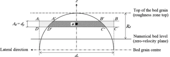
A schematic view of the bed drag force model including the roughness spheres is shown in Figure 3, in which the roughness zone is from the numerical bed level (zero-velocity plane) to the crest of the sphere with a thickness ofRd. Considering a section normal to theflow direction

as depicted in Figure 3, it is assumed that when afluid particle ais located within the roughness zone, the roughness element (the sphere) produces a drag-induced shear on this particle. This actually exerts a force on thefluid fragment of widthdsand heightdp(ABCDin Figure 3), whereds

is the diameter of the roughness sphere and dp is the computational particle size. Therefore, the

cross-sectional areaAdin Eq. (12) is assumed to be equal to the particle sizedp, and the bed-parallel

planar areaA_τin Eq. (11) is equal todsdp. Meanwhile, for eachfluid particle located in the

rough-ness zone, as depicted in Figure 3, a shape functionWdis defined as the area of part of the water

fragment located within the sphere (A′B′C′D′ in Figure 3) over the total area of the fragment (ABCD=dsdp) by the following equation:

Wd ¼

A_A′_B′_C′_D′ AABCD :

(20)

This function accounts for the shape of the roughness elements that are defined as spheres in the present study to match the roughness elements used in the laboratory study.

Another parameter of Eq. (12) that needs to be considered is the drag coefficientCd. According to

the original work on particle modelling of porousflows using the MPS method by Gotoh and Sakai [31],Cdusually lies between 1.0 and 1.5, and thus, a value of 1.0 is simply adopted in the present

study. Different values ofCdhave also been described in the literature for spherical particles. In the

experiments of Schmeeckleet al.[49] on turbulent open channelflow overfixed spheres, the drag coefficient was found to be 0.76. They also measured the drag force in turbulentflows over cubes and natural particles and found that the drag coefficient was significantly higher than that used to model the bed load motion. In the proposed drag force model (Eq. (12)), the product ofCdWdacts

as the total drag coefficient. By assuming half of the bed grain to be the effective roughness height andCd= 1.0, the average value ofCdWdfor the particles inside the roughness zone would be equal

to 0.785, which is close to the value found by Schmeeckleet al.[49] for spherical particles. Here, it should be noted that the roughness spheres as shown in Figure 3 do not physically exist in the nu-merical model so particles can penetrate inside the roughness zone but feel its influence.

3. MODEL APPLICATIONS AND RESULTS ANALYSIS

3.1. Model setup and computational parameters

In this section, an SPH model is developed for uniform turbulent open channelflows over a sloping rough bed and validated by the depth and velocity data obtained from Particle Image Velocimetry (PIV) measurement in a laboratory channel with uniform-sized spheres packed in a hexagonal

pattern on the bed [50]. In these tests, the bed sphere diameterdsis 24 mm, and the channel slopeS0

ranges from 0.002 to 0.004. For this application, a rectangular computational domain is chosen with a length ofL= 4H, whereHis the water depth. Three layers offixed dummy particles are used for the bottom wall, and three layers of moving particles are used for the inflow as well as outflow regions to satisfy the complete kernel area of the inner-fluid particles near the boundary lines (Figure 1). Because the effect of bottom roughness on theflow depends not only on the absolute roughness size but also on theflow conditions, 12 test cases with different bed slopes and water depths are simulated to assess the accuracy of the drag force model in addressing the roughness effect. Relevant parameters used in the test cases are summarized in Table I. According to this table, theFrnumber for all 12 cases is below 1, which means all tests are in the sub-criticalflow condi-tion, while Chang and Chang [34] and Changet al.[35] covered moreflow regimes. Meanwhile, the domain is discretized by SPH particles with sizedp= 2 mm to have at least 20 particles over

the depth for the shallowest case (H= 40 mm). The smoothing length is taken to be 1.2dpin the

present study. This value has been recommended as the most appropriate SPH smoothing length in many studies as common practice. Because the interfacial boundary layer in the physical model between the bed roughness and the freeflow is expected to be quite thin, a kernel function with a narrower influence domain but steeper slope near the central point is expected to be more adequate. Therefore, the cubic spline function of Monaghan and Lattanzio [51] is chosen for the present sim-ulations. However, an in-depth investigation is required for the choice of spatial resolution, smooth-ing length and kernel function in cases where theflow velocity changes sharply over an interfacial boundary layer as in the present study.

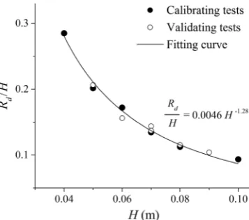
As illustrated in Table I, the model has been applied to differentflow conditions with bed slopes 0.002, 0.003 and 0.004, and water depths from 40 to 100 mm. As mentioned in the previous section, the thickness of the roughness zone (Rd) is assumed to vary depending on the flow conditions.

Therefore, six of the test cases (nos. 1, 5, 6, 8, 10 and 12) are used to calibrate the model in terms ofRdby numerical trials when the computed mean velocity profiles achieved the bestfit with the

experimental data and then a semi-empiricalfitting function is obtained to establish the relationship between theflow depth and relative roughness heightRd/H. Based on this, the additional test cases

(nos. 2, 3, 4, 7, 9 and 11) are used to validate the model. The calibration tests are selected to cover most of the depth range from 40 to 100 mm and at least two cases of each bed slope. Calibration and validation tests are indicated by letters C and V, respectively, in Table I.

The calibration process is as follows. Each test case is simulated by using severalRdvalues, and

the mean absolute error (MAE) between the numerical and experimental velocity profiles is calcu-lated for each one; then, theRdvalue corresponding to the minimum MAE is selected as the

thick-ness of the roughthick-ness zone for that test case. After running the model for calibrating tests and

finding the best Rdwith the smallest MAE, the relative roughness heightRd/His plotted against

depthH(Figure 4), and a curve isfitted to the points using a power function as shown in thefigure. For each validating case, different values ofRdare examined in the simulations, and the one with

Table I. Computational parameters used in test cases (thefirst four letters and numbers in the test ID show the bed slope, and the rest show the water depth).

Test no. Test ID S0 H(mm) u*(m/s) Re Fr Calibration/validation

1 S004H40 0.004 40 0.0396 10 843 0.433 C

2 S004H50 0.004 50 0.0443 15 067 0.430 V

3 S004H70 0.004 70 0.0524 32 703 0.564 V

4 S004H90 0.004 90 0.0594 47 301 0.559 V

5 S004H100 0.004 100 0.0626 59 698 0.603 C

6 S003H50 0.003 50 0.0384 11 615 0.332 C

7 S003H60 0.003 60 0.0420 19 516 0.424 V

8 S003H70 0.003 70 0.0454 27 926 0.481 C

9 S003H80 0.003 80 0.0485 32 089 0.453 V

10 S002H60 0.002 60 0.0343 12 022 0.261 C

11 S002H70 0.002 70 0.0371 19 671 0.339 V

the minimum MAE is used for the test case and plotted on the same graph to see if it follows the

fitted curve. As can be seen, theRd/Hvalues of the validation tests have nearly the same relation

with the water depth. Further evidence of the model validations will be demonstrated by the good agreement between the numerical and experimental velocity and shear stress distributions along the

flow depth, as detailed in the next section.

3.2. Analysis of velocity profiles

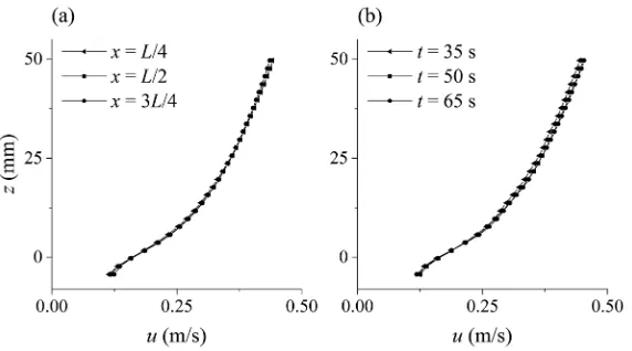
Figure 5(a) and (b) presents the instantaneous streamwise velocity and pressure (t= 70 s), and Figure 5(c) and (d) shows their time-averaged contours, respectively, for the case S004H50. The averaging has been performed over 20 s fromt= 70 to 90 s. It shows that the uniformflow condition has been successfully imposed by the proposed inflow/outflow boundary technique. This is also shown in Figure 6(a) where the time-averaged velocity of three different sections of the channel (x= 0.25L, 0.50Land 0.75L) are plotted. It is found that the depth-averaged velocity at these three sections has a maximum difference of 0.5%. Figure 6(b) shows the space-averaged velocity at three different times (t= 35, 50 and 65 s). The maximum difference of the depth-averaged velocity be-tween these times is 1.96%. This small change in the velocity profile over time also shows the steadiness of theflow. In the present computations, the time to reach the steady state is not exactly the same for all test cases. However, to determine a threshold, it is confirmed that it takes around 20–30 s to achieve the steadyflow condition for all 12 cases. The criterion used to define if theflow

Figure 4. Calibration and validation of the model in terms of the effective roughness height versus the water depth.

reaches the steady state is that if the differences of the depth-averaged value of the space-averaged (but not instantaneous) velocities at the mid-section of the channel at different times become less than 2.0%, then theflow is regarded as being steady. The bed drag-induced shear term removes a part of theflow momentum, and this effect is transferred to the upper layers of the flow by the turbulence model. As a result, the unbalanced momentum transfer occurs during thefirst 20–30 s, and then the flow gradually reaches the steady state and all time-averaged flow parameters, for example, velocity and shear stress remain unchanged. In the inflow and outflow boundaries, the

flow characteristics are assumed to be unknown rather than being given prescribed values of the pressure and velocity. Therefore, the proposed SPH inflow boundary model is more general in that it does not need experimentally measured or analytically prescribedflow data at the inflow bound-ary and can thus be applied to more complexflow situations. In Federicoet al.[22], the model ver-ification was based on the fact that the initial inner velocityfield, which was initialized with the analytical solutions and updated by the upstream inflow boundary condition (which was also initial-ized by the analytical solutions), could be stably maintained or not during the computations. In comparison, in the present SPH inflow model, the open channelflows are generated naturally by following the channel conditions.

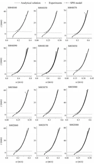
The numerical results of time-averaged streamwise velocity profiles obtained by using the best-fit values ofRdare presented in Figure 7, in comparison with the experimental data as well as the

an-alytical profiles that are obtained from the log law. These include all the test cases as indicated in Table I. The analytical velocity profile is presented in Eq. (21) where zis vertical coordinate, ks

is the Nikuradse roughness size and Bris the logarithmic integration constant that is equal to 8.5

for rough bed uniformflow. We know that as the depth is very shallow and the bed is fully rough, the log law may not be valid. Here, the analytical profiles are used to compare with the numerical results and investigate if the model is able to predict the logarithmic velocity distribution above the roughness zone. The values ofRdas well as MAE of velocity profiles of all test cases are presented

in Table II. Both Figure 7 and Table II demonstrate the satisfactory performance of the SPH model-ling technique in these proposedflow conditions.

u u¼

1

kln z ks

þBr: (21)

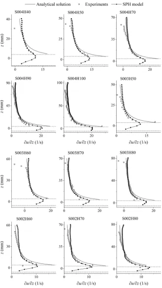
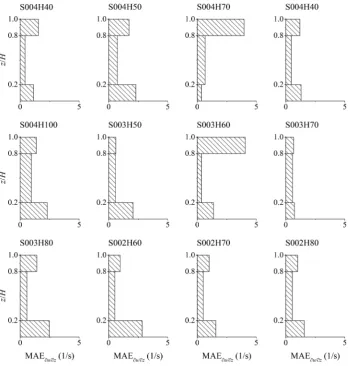
To determine the error distribution over depth, the MAE is calculated separately in three parts of the depth for each test case, that is, lower 20%, middle 60% and upper 20% of the depth. The pur-pose of this is to investigate the hypothesis [50] that the bottom 20% of the water depth would be the logarithmic layer and then the upper layers of the flow could be split up differently. This is shown in Figure 8. As the slope of the velocity profile (∂u/∂z) is also of interest, its distribution

is presented in Figure 9 for all test cases, and the values of MAE of these profiles are also calcu-lated. The MAE values of ∂u/∂z are presented in Table II, and their distributions in the lower 20%, middle 60% and upper 20% of the depth for all cases are illustrated in Figure 10.

According to Figure 8, with increasing depth, the velocity MAE of the upper 20% of the depth mostly increases, and as the slope decreases, the MAE of the near-bed velocity generally increases. In most test cases, the lowest MAE of the velocity profiles takes place in the middle part of the depth. This is also valid for the MAE of the velocity gradient profiles as can be seen in Figure 10. Compared with the velocity, the errors of the velocity gradient are usually larger in

Table II. Relative roughness heights and numerical errors of all tests.

Test no. Test ID Rd/H MAE ofu(m/s) MAE of∂u/∂z(1/s)

1 S004H40 0.285 0.0052 0.77

2 S004H50 0.206 0.0060 1.17

3 S004H70 0.144 0.0100 1.27

4 S004H90 0.104 0.0100 0.77

5 S004H100 0.094 0.0179 1.25

6 S003H50 0.202 0.0047 1.40

7 S003H60 0.156 0.0063 1.39

8 S003H70 0.135 0.0078 0.67

9 S003H80 0.116 0.0080 1.11

10 S002H60 0.172 0.0052 1.05

11 S002H70 0.137 0.0061 0.81

12 S002H80 0.113 0.0061 0.82

MAE, mean absolute error.

Figure 9. Distribution of the gradient of the time-averaged streamwise velocity over depth. Dash-dotted and dashed lines show the level of the numerical bed (zero-velocity plane) and the crest of the roughness zone,

the lower 20% of the depth. However, in some cases (e.g. S004H70 and S003H60), there seems to be a large error in the upper part of the depth due to the fact that the predicted and measured gradients have different signs near the water surface. Just below the surface, the experimental velocity gradient declines sharply to 0 or even to negative values in some cases, while a non-zero, but small positive velocity gradient is predicted by the numerical model (Figure 9). The negative gradient in the top of the flow could be due to the fact that the data are derived from a 3D experimental model in which secondaryflow circulations occur, while such circulations are not accounted for in the present 2D numerical model. However, the log law (Eq. (21)) presents a positive small, but non-zero velocity gradient at the top (Figure 9), which is much more sim-ilar to the numerical profiles than the experimental ones. This is because the mixing-length model (Eq. (9)) adopted by the SPH approach has been based on the log law theory. In the mixing-length formula of Nezu and Rodi [41], it is assumed that above a certain elevation, the mixing length decreases to 0 at the water surface as the size of turbulent eddies is signifi -cantly restricted by the surface. Assuming such a decline in the mixing length could lead to a non-zero velocity gradient near the water surface. On the other hand, the differences in the near-bed velocity gradient between the numerical and experimental profiles are much less than those between the analytical and experimental ones. This is attributed to the adoption of the ro-bust drag force model by which the near-bed velocity is related to the shear from the roughness elements rather than assuming a logarithmic distribution in the shear boundary.

3.3. Analysis of roughness height

During the calibration/validation process (Section 3.1), theRdvalues corresponding to the

mini-mum errors, if divided by the water depth, showed a relationship with the depth based on the power function as presented in Figure 4. According to this figure, as the depth increases, the relative roughness height (Rd/H) decreases. It is notable that the bed roughness sphere size isfixed in the

present study (ds= 24 mm). Therefore,Rd/Hdecreases with a decrease in the ratio of roughness size

to water depth (ds/H) and vice versa. In this work, the bed roughness configuration is kept constant

to study its effect under differentflow conditions. As the depth is not the only parameter affecting theflow condition and the bed slope is also involved, we also explored the relationship between the relative roughness height (Rd/H) and the shear velocityu*. The result is shown in Figure 11(a) with

different powerfitting functions for different bed slope values. It is shown that thefitting curves are nearly equally spaced with a vertical shift upwards as the bed slope increases and the SPH compu-tational points fall close to the appropriate curves.

It can also be seen that an increase in the shear velocity causes the numerical relative roughness height to become milder for all bed slopes. To provide a single relationship between the relative roughness height and the flow condition, Rd/S0H of all cases are plotted againstu*in Figure 11

(b) with the same type of power fitting curve. This also shows that as the flow becomes more sheared (largeru*), smaller relative roughness height is required to simulate the experimental

con-dition. In other words, as the ratio of bed roughness to water depth (ds/H) becomes smaller, that is,

when theflow depth becomes deeper, a weaker bed effect is generated by the proposed drag force model. However, the magnitude of the form-drag shear term could be larger for the cases with higheru*because the near-bedflow velocity is faster.

3.4. Analysis of form-drag and turbulent shear stress

The distribution of the streamwise form-drag shear term (τd/ρ) in the effective roughness zone is

presented in Figure 12 for all the tests. As expected, the averageτd/ρis larger for cases with higher

u*orRenumber. In other words, where theflow depth is deeper and/or the bed slope is steeper, the

form-drag shear term is larger because of the higher velocity. In most tests, the streamwiseτd/ρ

increases with depth to some distance above the wall (zero-velocity plane) and then decreases to the crest of the roughness zone although the velocity increases in this zone. This decrease can be the result of the shape function in Eq. (20) that declines sharply below the roughness crest. The shape function leads to a non-constant drag coefficient in the roughness zone that is related to the shape of the elements. In the present simulations, the dominant velocity is the streamwise one, and the contribution of the vertical velocity to the form drag is very small so that it is reasonable to be neglected. It has been found that in the roughness zone, the scale of the time-averaged vertical velocity is less than 0.5% of the time-averaged streamwise velocity in our test cases, while it is

Figure 11. Relative roughness height against shear velocity: (a) relationship betweenRd/Handu*for

about 1.0% to 2.0% in the presented 3D experimental data. The underestimation of the vertical ve-locity in the roughness zone could be due to that the physical dispersion in the vertical direction that is from the obstruction of theflow by the bed elements has not been numerically defined, because the governing equations and the computational domain are discretized at a macroscopic scale. In Figure 13, the numerical results of the streamwise velocity profiles of tests of bed slope 0.004, 0.003 and 0.002 are plotted in separate graphs in order to illustrate the effect of rough bed boundary on the streamwiseflow velocity. As can be seen for each bed slope, the velocity is higher for larger depths, and this effect is simulated by variable roughness height in the model.

Using a variableRdin the model affects not only the drag shear term but also the turbulent shear

stress near the bed. In the present model, the zero reference datum for the mixing length is defined by the zero-velocity plane of theflow. This is illustrated in Figure 14 wherelm is plotted for two

cases with effective roughness heights of Rd,1and Rd,2(Rd,2>Rd,1). Here, the eddy-viscosity is

higher when the thickness of the roughness zone (Rd) is larger; thus, the shear stress calculated

by Eq. (4) is also larger. This leads to a higher impact of the bottom drag effect on the upperflow. In general, any changes ofRdcould affect both the drag force and the turbulence models, and thus,

the simulatedflows will change. It is also notable that a small change in the mixing length, on the crest of the roughness zone, could have a considerable effect on the eddy-viscosity (Eq. (8)) because the velocity gradient (or the local strain rate |S|) is at a maximum on this interface.

For six of the 12 test cases shown in Table I, the profiles of the time-averaged shear stress esti-mated by the SPS with the mixing-length model are presented in Figure 15 in comparison with the experimental data and with the analytical profile obtained from Eq. (22). In this equation,τ0is the

shear stress at the bed that is estimated byρgHS0.

Figure 12. Distribution of the drag-induced shear term in the effective roughness zone (solid line). Dash-dotted and Dash-dotted lines show the level of the numerical bed (zero-velocity plane) and the crest of the

Figure 13. Velocity profiles of tests with bed slopes (a) 0.004, (b) 0.003 and (c) 0.002. The dashed lines show the level of the roughness crest, and the solid half circles schematically depict the roughness element.

Figure 14. Distribution of the mixing length in two cases with the same depth (H= 50 mm) and different effective roughness heights (Rd,2>Rd,1). The zero reference of the mixing length is on the numerical bed

level (zero-velocity plane), and the dotted line shows the crest of the roughness zone.

τ¼τ0 1 z H

: (22)

To better illustrate the data, the horizontal axis is normalized byτ0, and the vertical one is

nor-malized by theflow depthH. As can be seen, the numerical computations underestimate the exper-imental shear stresses, although they are in a fairly good agreement with the analytical solution. It is notable that the experimental data are taken from a 3Dflow over a rough bed surface, which could lead to that they exceed the analytical shear stresses by about 20–30%. Besides, the underestimation of the experimental shear stress by the numerical model is also related to the dimensional differ-ences, as in the present 2D model, the shear stress in the lateral direction is neglected. The width-wise shear stress is the result of steady streaming in the form offlow circulations in the lateral direction. In spite of this, the 2D SPS model is still able to give satisfactory results in the uniform

flow because the effect of the lateral shear stress is very much smaller compared with the streamwise one. Moreover, the close collapses of six SPH data along almost a single line indicate the consistency and convergence of the numerical simulations.

As mentioned before, the eddy-viscosity model with a Smagorinsky constant in the range of 0.1– 0.15 is not able to estimate the correct amount of turbulent shear stress in a uniform open channel

flow over a rough bed boundary. To investigate this issue, here, we repeat the simulations of three test cases S004H50, S003H70 and S002H60 by using the Smagorinsky model withCs= 0.15. The

result is presented in Figures 16 and 17, where, respectively, the streamwise velocity and shear stress profiles are compared with the ones obtained from the present mixing-length eddy-viscosity model. Meanwhile, the experimental velocity profiles and the analytical shear stress profiles are also presented for a comparison. As can be seen, the shear stress is consistently largely underestimated, leading to the overestimation of the velocity.

In contrast to their DNS results with good agreement with the reference data, Mayrhoferet al.

[37] observed the overestimation of the velocity in their SPH-LES computations of a wall-bounded channelflow with frictionReof 1000, where an eddy-viscosity model was used with a Smagorinsky constant Cs= 0.065. They pointed out that the correct representation of energy redistribution

be-tween Reynolds stress components in an SPH-LES framework would require 16 timesfiner resolu-tion than needed in a classic Eulerian LES one. They stated that the most obvious soluresolu-tion is an increase in the resolution but it also highly increases the computational cost. Finally, they concluded that the underperformance of their LES was due to the problems inherent in the standard SPH discretizations related to the pressure–velocity interactions.

Figure 16. Time-averaged streamwise velocity obtained from the present mixing-length model compared with the one obtained from the Smagorinsky model withCs= 0.15 and the experimental data for test cases

In the present study, the frictionReis even higher than that in the study of Mayrhoferet al.[37], and on the other hand, the resolution is also quite coarse. Therefore, the insufficiency of the LES with the standard Smagorinsky model becomes more obvious in the present simulations. In addition, the rough bed boundary is another important influence factor too. When filtering the discretized equations using an SPH kernel function to represent the turbulence effect, a part of the turbulent stress that is mainly due to the spatial filtering has been lost by the standard eddy-viscosity model (with Smagorinsky constant). This issue becomes even more important when the discretizedflow velocity changes sharply over the filtering volume/area, for example, at the interfacial boundary between the roughness zone and the freeflow in the present study. Besides, the rough bed boundary has a dominant effect on the whole water depth, so non-accurate parameterization of the turbulence effect at this boundary makes significant errors in the wholeflow domain. However, if the eddy-viscosity model is adequately parameterized, reasonable results can still be obtained. As a result, we have applied the mixing-length model of Nezu and Rodi [41], which is on the basis of physical measurements, in order to recover that part of the turbulent stress that cannot be captured by the standard Smagorinsky model with smallCs.

Nonetheless, one shortcoming of the proposed turbulence model is that the eddy-viscosity coefficient is physically defined so it is not dependent on the computational resolution. In other words, if one uses a smaller particle size (higher resolution), the resolved part of the turbulence stress would become higher, but the mixing-length product that is the representative of the unresolved part would not decrease with the discretization and/orfiltering size. Thus, the total turbulent stresses could be overestimated in the cases with higher resolution. Accordingly, theflow velocities would be ex-pected to be underestimated in such a situation. It is promising to note that the present mixing-length approach works quite effectively with the SPH when relatively coarse particle resolution is used, which is the case in most practical engineering applications.

4. CONCLUSION

In this study, an SPH model has been developed to simulate the turbulent open channelflows over rough bed boundaries based on the solution of 2D N-S equations including two additional stress terms to account for the flow turbulence and bed roughness effect. As shown, the standard Smagorinsky-based SPS model with a fixedCs= 0.15 was unable to reproduce the correct shear

mechanisms in uniform open channelflows. Therefore, a mixing-length model has been applied to calculate the turbulent eddy-viscosity. A drag force model has been developed to account for the bed roughness effect, in which a shape function is introduced to consider the geometry of the bed surface roughness elements. Meanwhile, an efficient inflow/outflow boundary treatment has

Figure 17. Thex-zcomponent of the turbulent shear stress obtained from the present mixing-length model compared with the one obtained from the Smagorinsky model withCs= 0.15 and the analytical profiles for

been proposed and demonstrated to generate a stable flow simulation without the need to use prescribed velocities at theflow inlet.

Twelve test cases of different bed slopes and water depths have been simulated to investigate the effect of bed roughness under variousflow conditions. A roughness zone is defined near the rough bed boundary where a form-induced drag shear term is applied on the SPH particles. The thickness of this zone (Rd) is assumed to be flow dependent, such as being related to the flow

depth H and the shear velocity on bed u*. The model results showed good agreement with the

experimental data as well as the analytical solutions in view of the velocity and shear stress

pro-files. This confirms that the bed roughness effect has been successfully addressed by the drag force model and the transport of this effect to the upper layers of the flow has been correctly reproduced by the proposed turbulent mixing-length approach. Because the governing equations, as well as the computational domain, are discretized at a macroscopic scale in the roughness zone, the physical dispersion in the vertical direction is disregarded. Thus, the flow shear is dominantly driven in the streamwise direction but transported vertically by the turbulence clo-sure. The computed streamwise velocity and shear stress profiles suggested that this assumption has not caused substantial errors for the 12 flow test cases and the macroflow behaviours have been well reproduced. This is due to the turbulence model correctly modelling the shear transfer from the roughness layer to the free flow.

Whether the inaccuracy of the SPH-LES approach in wall-bounded channelflows is related to the pressure–velocity interactions (as addressed by [37]) or to the deficiency of the standard Smagorinsky model, the proposed mixing-length approach is able to overcome this difficulty due to the eddy-viscosity being realistically parameterized. However, as the mixing length is indepen-dent of the computational resolution, it may overestimate the shear stress in cases with higher particle resolution that may cause an underestimation of the flow velocity. Therefore, this model is proposed to be coupled with the SPH when coarse discretization of the equations is considered, unless an effective method is found to link the mixing length to the spatial discretization so as to enhance the capacity of the model. In addition to this, the method of filtering the governing equations with different kernel functions needs to be investigated in more detail because of the existence of the rough bed boundary over which theflow velocity has a sharp change. These issues along with the effect of various configurations of bed roughness on theflow resistance are consid-ered as future studies.

ACKNOWLEDGEMENTS

This work was supported by the Research Executive Agency, through the 7th Framework Programme of the European Union, Support for Training and Career Development of Researchers (Marie Curie-FP7-PEOPLE-2012-ITN), which funded the Initial Training Network (ITN) HYTECH ‘Hydrodynamic Transport in Ecologically Critical Heterogeneous Interfaces’, No. 316546. The experimental work was supported by EPSRC (Grant No. EP/G015341/1).

REFERENCES

1. Nikora V, Koll K, McEwan I, McLean S, Dittrich A. Velocity distribution in the roughness layer of rough-bed

flows.Journal of Hydraulic Engineering2004;130:1036–1042.

2. Nicholas AP. Computationalfluid dynamics modelling of boundary roughness in gravel-bed rivers: an investigation of the effects of random variability in bed elevation.Earth Surface Processes and Landforms2001;26:345–362. 3. Smagorinsky J. General circulation experiments with the primitive equations. I. The basic experiment. Monthly

Weather Review1963;91:99–164.

4. Van Driest ER. On turbulentflow near a wall.Journal of the. Atmospheric Sciences1956;23:1007–1011. 5. Rotta J. Turbulent boundary layers in incompressibleflow.Progress in Aerospace Sciences1962;2:73–82. 6. Cebeci T, Chang KC. Calculation of incompressible rough-wall boundary-layer flows.AIAA Journal1978;16

(7):730–735.

7. Christoph GH, Pletcher RH. Prediction of rough-wall skin friction and heat transfer. AIAA Journal 1983;

21:509–515.

9. Wiberg PL, Smith JD. Velocity distribution and bed roughness in high-gradient streams.Water Resources Research 1991;27:825–838.

10. Cui J, Patel VC, Lin CL. Prediction of turbulentflow over rough surfaces using a force field in large eddy simulation.Journal of Fluids Engineering ASME2003;125:2–9.

11. Carney SK, Bledsoe BP, Gessler D. Representing the bed roughness of coarse grained streams in computational

fluid dynamics.Earth Surface Processes and Landforms2006;31:736–749.

12. Zeng C, Li CW. Modelingflows over gravel beds by a drag force method and a modified S–A turbulence closure. Advances in Water Resources2012;46:84–95.

13. Gotoh H, Shao S, Memita T. SPH-LES model for numerical investigation of wave interaction with partially immersed breakwater.Coastal Engineering Journal2004;46(1):39–63.

14. Shao S, Gotoh H. Simulating coupled motion of progressive wave andfloating curtain wall by SPH-LES model. Coastal Engineering Journal2004;46(2):171–202.

15. Shao S, Gotoh H. Turbulence particle models for tracking free surfaces.Journal of Hydraulic Research2005;43 (3):276–289.

16. Khayyer A, Gotoh H. Enhancement of stability and accuracy of the moving particle semi-implicit method.Journal of Computational Physics2011;230(8):3093–3118.

17. Lind SJ, Xu R, Stansby PK, Rogers BD. Incompressible smoothed particle hydrodynamics for free-surfaceflows: a generalised diffusion-based algorithm for stability and validations for impulsive flows and propagating waves. Journal of Computational Physics2012;231:1499–1523.

18. Gotoh H, Khayyer A, Ikari H, Arikawa T, Shimosako K. On enhancement of incompressible SPH method for simulation of violent sloshingflows.Applied Ocean Research2014;46:104–115.

19. Ferrand M, Laurence DR, Rogers BD, Violeau D, Kassiotis C. Unified semi-analytical wall boundary conditions for inviscid, laminar or turbulentflows in the meshless SPH method.International Journal for Numerical Methods in Fluids2013;71:446–472.

20. Leroy A, Violeau D, Ferrand M, Kassiotis C. Unified semi-analytical wall boundary conditions applied to 2-D incompressible SPH.Journal of Computational Physics2014;261:106–129.

21. Tsuruta N, Khayyer A, Gotoh H. Space potential particles to enhance the stability of projection-based particle methods.International Journal of Computational Fluid Dynamics2015;29(1):100–119.

22. Federico I, Marrone S, Colagrossi A, Aristodemo F, Antuono M. Simulating 2D open-channelflows through an SPH model.European Journal of Mechanics - B/Fluids2012;34:35–46.

23. Fu L, Jin YC. A mesh-free method boundary condition technique in open channelflow simulation. Journal of Hydraulic Research2013;51(2):174–185.

24. Gotoh H, Shibahara T, Sakai T. Sub-particle-scale turbulence model for the MPS method–Lagrangianflow model for hydraulic engineering.Computational Fluid Dynamics Journal2001;9:339–347.

25. Violeau D, Issa R. Numerical modelling of complex turbulent free-surfaceflows with the SPH method: an overview. International Journal for Numerical Methods in Fluids2007;53(2):277–304.

26. Lopez D, Marivela R, Garrote L. Smoothed particle hydrodynamics model applied to hydraulic structures: a hydraulic jump test case.Journal of Hydraulic Research2010;48:142–158.

27. Sahebari AJ, Jin YC, Shakibaeinia A. Flow over sills by the MPS mesh-free particle method.Journal of Hydraulic Research2011;49(5):649–656.

28. Chern M, Syamsuri S. Effect of corrugated bed on hydraulic jump characteristic using SPH method.Journal of Fluids Engineering ASME2013;139(2):221–232.

29. De Padova D, Mossa M, Sibilla S, Torti E. 3D SPH modelling of hydraulic jump in a very large channel.Journal of Hydraulic Research2013;51(2):158–173.

30. Arai J, Koshizuka S, Murozono K. Large eddy simulation and a simple wall model for turbulentflow calculation by a particle method.International Journal for Numerical Methods in Fluids2013;71:772–787.

31. Gotoh H, Sakai T. Lagrangian simulation of breaking waves using particle methods.Coastal Engineering Journal 1999;41(3&4):303–326.

32. Khayyer A, Gotoh H. Modified moving particle semi-implicit methods for the prediction of 2D wave impact pressure.Coastal Engineering2009;56(4):419–440.

33. Khayyer A, Gotoh H. On particle-based simulation of a dam break over a wet bed.Journal of Hydraulic Research 2010;48(2):238–249.

34. Chang TJ, Chang KH. SPH modeling of one-dimensional nonrectangular and nonprismatic channelflows with open boundaries.Journal of Fluids Engineering ASME2013;139(11):1142–1149.

35. Chang TJ, Chang KH, Kao HM. A new approach to model weakly nonhydrostatic shallow waterflows in open channels with smoothed particle hydrodynamics.Journal of Hydrology2014;519(A):1010–1019.

36. Chang TJ, Kao HM, Chang KH, Hsu MH. Numerical simulation of shallow-water dam breakflows in open channels using smoothed particle hydrodynamics.Journal of Hydrology2011;408(1-2):78–90.

37. Mayrhofer A, Laurence D, Rogers BD, Violeau D. DNS and LES of 3-D wall-bounded turbulence using smoothed particle hydrodynamics.Computers & Fluids2015;115:86–97.

38. Mayrhofer A, Rogers BD, Violeau D, Ferrand M. Investigation of wall boundedflows using SPH and the unified semi-analytical wall boundary conditions.Computer Physics Communications2013;184(11):2515–2527. 39. Kazemi E, Tait S, Shao S, Nichols A. Potential application of mesh-free SPH method in turbulent riverflows.

40. Cheng NS, Nguyen HT, Tan SK, Shao S. Scaling of velocity profiles for depth-limited open channelflows over submerged rigid vegetation.Journal of Hydraulic Engineering2012;138(8):673–683.

41. Nezu I, Rodi W. Open-channel flow measurements with a laser Doppler anemometer. Journal of Hydraulic Engineering1986;112(5):335–355.

42. Coles D. The law of the wake in the turbulent boundary layer.Journal of Fluid Mechanics1956;1:191–226. 43. Coleman NL. Velocity profiles with suspended sediment.Journal of Hydraulic Research1981;19:211–229. 44. Gingold RA, Monaghan JJ. Smoothed particle hydrodynamics: theory and application to non-spherical stars.

Monthly Notices of the Royal Astronomical Society1977;181(3):375–389.

45. Monaghan JJ. On the problem of penetration in particle methods.Journal of Computational Physics1989;

82(1):1–15.

46. Aristodemo F, Marrone S, Federico I. SPH modeling of plane jets into water bodies through an inflow/outflow algorithm.Ocean Engineering2015;105:160–175.

47. Tan SK, Cheng NS, Xie Y, Shao S. Incompressible SPH simulation of open channelflow over smooth bed.Journal of Hydro-Environment Research2015;9(3):340–353.

48. Hosseini SM, Feng JJ. Pressure boundary conditions for computing incompressibleflows with SPH.Journal of Computational Physics2011;230:7473–7487.

49. Schmeeckle MW, Nelson JM, Shreve RL. Forces on stationary particles in near-bed turbulentflows.Journal of Geophysical Research2007;112:F02003.

50. Nichols A. Free surface dynamics in shallow turbulentflows. 2013. PhD thesis, School of Engineering, University of Bradford, UK.

51. Monaghan JJ, Lattanzio JC. A refined method for astrophysical problems. Astronomy & Astrophysics 1985;