This is a repository copy of Time-dependent probability density function in cubic stochastic processes.
White Rose Research Online URL for this paper: http://eprints.whiterose.ac.uk/108219/
Version: Accepted Version
Article:
Kim, E-J. and Hollerbach, R. (2016) Time-dependent probability density function in cubic stochastic processes. Physical Review E, 94 (5). ISSN 2470-0045
https://doi.org/10.1103/PhysRevE.94.052118
Reuse
Unless indicated otherwise, fulltext items are protected by copyright with all rights reserved. The copyright exception in section 29 of the Copyright, Designs and Patents Act 1988 allows the making of a single copy solely for the purpose of non-commercial research or private study within the limits of fair dealing. The publisher or other rights-holder may allow further reproduction and re-use of this version - refer to the White Rose Research Online record for this item. Where records identify the publisher as the copyright holder, users can verify any specific terms of use on the publisher’s website.
Takedown
If you consider content in White Rose Research Online to be in breach of UK law, please notify us by
This is a Time-dependent probability density function in cubic stochastic processes
Article:
! ∀# ∃%& ∋ ( # ) ∗ ∀ % ( ( + + (
, + ∃ −../ 01 % 02 )− , ∗
( , +
∃ ( 3 % 4 +
Time-Dependent Probability Density Function in Cubic
Stochastic Processes
Eun-jin Kim
School of Mathematics and Statistics, University of Sheffield, Sheffield, S3 7RH, U.K.
Rainer Hollerbach
Department of Applied Mathematics, University of Leeds, Leeds, LS2 9JT, U.K.
Abstract
We report time-dependent Probability Density Functions (PDFs) for a nonlinear stochastic
pro-cess with a cubic force by novel analytical and computational studies. Analytically, a transition
probability is formulated by using a path integral and is computed by the saddle-point solution
(instanton method) and a new nonlinear transformation of time. The predicted PDF p(x, t) is in
general given as a time integral and useful PDFs with explicit dependence onxandtare presented in certain limits (e.g. in the short and long time limits). Numerical simulations of the
Fokker-Planck equation provide exact time evolution of the PDFs and confirm analytical predictions in the
limit of weak noise. In particular, we show that non-equilibrium PDFs behave drastically differently
from the stationary PDFs in regards to the asymmetry (skewness) and kurtosis. Specifically, while
stationary PDFs are symmetric, transient PDFs are skewed; transient PDFs are much broader
than stationary PDFs, with the kurtosis larger and smaller than 3, respectively. We elucidate the
I. INTRODUCTION
Many systems in nature or laboratories not only involve stochastic processes due to
intrinsic variability, or to uncertainty in the system, but may also be far from equilibrium.
Computing the time-evolution of the probability density function (PDF) of such systems
is often a major challenge. While in thermal equilibrium the same level of fluctuations
can be maintained by a reservoir (e.g. heat bath) at a fixed temperature (e.g. by the
fluctuation-dissipation theorem [1]), far from equilibrium there no longer exists such a
reservoir. The level of fluctuations in the system thus changes with time and becomes a
dynamical variable itself. For instance, drastic change in fluctuations can be caused by a
sudden change in the temperature at the reservoir, or just by an initial out-of-equilibrium
PDF. Consequently, a full knowledge of the time evolution of PDFs becomes critical.
As a simplest model, a Gaussian process has been widely used to understand a variety of
stochastic processes [2, 3]. At the heart of a Gaussian process is Brownian motion (random
walk) driven by white noise (random noise with a very short memory), where mean square
displacement increases linearly with time while there is no change in mean displacement.
When subject to a linear force, it becomes the Ornstein–Uhlenbeck (O-U) process, which
is a prototypical model for a noisy relaxation system, heavily used and extended in many
areas of physical science and financial mathematics (e.g. [2, 3]). This model is governed by
the following Langevin equation for a random variable x(say, the position):
dx
dt =−
∂V
∂x +ξ, (1)
where a linear force ∂V∂x = µox is given by a quadratic potential V(x) = µox2/2. Here, µo
is a non-negative constant andξ is the white noise characterised by the following statistical
property:
hξ(t)ξ(t′)i=Dδ(t−t′), (2)
where D is a constant. The angular brackets in Eq. (2) represent the ensemble average
over the noise. Given the initial condition (initial PDF), the time evolution of the PDF in
the subsequent time is precisely known as the joint distribution with a Gaussian transition
PDF of x, call itp(x, t), has the following time-evolution:
p(x, t) =
r
β πe
−β(x−hxi)2
, (3)
where hxi is the mean position, andβ is the inverse temperature given as:
hxi=x0e−µot,
1
2β =h(x− hxi)
2
i= D(1−e−
2µot)
2µo
, (4)
In a long time limit, a PDF approaches a stationary Gaussian distribution where the variance
of the PDF is set by hx2i =D/2µ
o. This stationary distribution can be linked to
thermo-dynamic equilibrium distribution by fluctuation–dissipation theorem by using 12hx2i = 1 2T
(with the Boltzmann constantkB= 1) and Eq. (4) as t → ∞as follows:
T = 1
2β(t → ∞) =
D 2µo
, (5)
which is the Einstein’s relation. We note that a factor of 1/2 in the last term in Eq. (4) and
(5) is due to our definition ofDin Eq. (2); that is, conventionally, Eq. (2) is defined with 2D
instead of D. For small time, the effect of the linear force is negligible compared to dxdt and the second equation in Eq. (4) recovers the usual Brownian motion with h(x− hxi)2i ∝ t.
For large time, the linear force becomes important, leading to the approach to the stationary
PDF. Mathematically, a Gaussian process offers a great analytical tractability in
comput-ing various statistical quantities (e.g. all even moments determined by second moments, etc).
Gaussian statistics however has serious limitations in explaining emerging complex
phe-nomena such as anomalous transport (super/sub diffusion), intermittency, self-organisation
or phase transition where a long-range correlation plays a key role [4–21]. In fact,
non-Gaussian PDFs often observed in these systems have stimulated an active research
on non-equilibrium statistics by considering nonlinear interaction, finite-correlated or
Levy-flight noise, multiplicative noise, fractional calculus, etc. (e.g. see [4–15, 17, 19–23]).
The main aim of this paper to shed light on this issue by elucidating the role of nonlinear
interaction in long-range correlation during the relaxation process of an initial PDF to a
final stationary PDF as an example of non-equilibrium processes.
To gain the key insight, it is valuable to consider the simplest nonlinear version of Eq.
results with the O-U process (e.g. Eq. (3)). To this end, we consider a cubic nonlinear
force (∝ x3) for a quartic potential V(x) = µx4/4 in Eq. (1) while keeping the same
short-correlated noise ξ given in Eq. (2). The cubic force has in fact been widely used
to model enhanced diffusion in various systems, including mixing in stellar interiors (e.g.
[24]) and self-organisation of shear flow by generalising a sand-pile in a continuous limit
[14, 20, 25]. In particular, [20] showed that similar stationary PDFs are obtained from 0D
dynamical model, 1D and 2D fluid models. This suggests important implications of the
results from a Langevin equation with cubic nonlinearity for a broad range of other physical
problems with the same highest nonlinearity.
For the cubic process, the prediction of time-dependent PDFs has proven to be elusive
[2]. However, a stationary distribution can easily be shown to be a quartic exponential PDF
p(x, t) = N e−βx4
where N ∝ β−1/4 (see Appendix A for its property), to which any initial
PDF relaxes in the long time limit. In this paper, we report on time-dependent PDFs
by novel analytical and computational studies. Analytically, a path integral formulation
[12, 14–16, 21, 26–33] and a nonlinear time transformation are utilised to predict a transition
probability. The PDF given in the path integral is computed by the saddle-point solution
(instanton method) (e.g. see [14–16, 21, 27–29, 31, 32]). The predicted p(x, t) in general
involves a time integral, and useful time-dependent PDFs with the explicit dependence on
x and t are presented in certain limits (e.g. in the short and long time limits). Numerical
simulations of the Fokker-Planck equation present detailed evolution of the time-dependent
PDF and confirm our analytical predictions.
We note that instantons originated in quantum mechanics as a non-perturbative way
of computing the transition amplitude from one ground state to another. The basic
idea is that the uncertainty relationship between position and momentum allows one to
formulate the transition amplitude from the initial to the final position by a path, and
the transition amplitude from one ground state to another can be isolated by considering
Euclidean action by taking time to be imaginary. An instanton is a saddle-point solution
of Euclidean action and corresponds to one particular path that leads to the transition
amplitude between ground states and was used in gauge field theory to compute the
was adapted to a classical fluid problem [32] and to a plasma problem [14–16]. In particular,
[27–29] reported a series of detailed calculations for (multi)-instantons for double wells
and different anharmonic potentials in quantum mechanics. [14–16] utilised it to predict
stationary PDF tails of anomalous transport due to large events by taking a long-time
limit, while [21] generalised this methodology to predict the time-dependent PDF for
the O-U process without taking such long-time limit. It is the purpose of this paper to
extend this work further to nonlinear stochastic processes. The unique contribution of
this work lies in the prediction of the time-dependent PDFs p(x, t) by calculating the
in-stanton solutions which satisfy the boundary conditions at the initial and final times (see§2).
The remainder of the paper is as follows. We present the path integral solution of PDFs
in Section II. Exact time-dependent PDF by simulations are provided in Section III. Section
IV contains discussions and conclusions.
II. ANALYTICAL PREDICTION
We consider the evolution of a random variablexunder a quartic potentialV(x) =µx4/4
in Eq. (1) and a white noise given by Eq. (2) as: dx
dt =−µx
3+ξ, (6)
whereµis the frictional constant for the cubic force. To gain a key insight into the evolution
of this system, it is useful to obtain the equation for the mean and fluctuating components
ofx by lettingx=hxi+δxin Eq. (6). Here, hxiandδx are the mean value and fluctuation
so that hδxi= 0. Then, the time evolution of hxi and δx can easily be shown to be as dhxi
dt = −µ
(hxi2+h(δx)2i)hxi+h(δx)3i
, (7)
dδx
dt = −3µhxi
2δx+G+ξ, (8)
where G = 3hxi[(δx)2 − h(δx)2i] + (δx)3 − h(δx)3i. For small fluctuation, we can apply
the quasi-linear analysis to ignore G and h(δx)3i in Eqs. (7)–(8) and obtain approximate
equations:
dhxi
dt = −µ
hxi2+h(δx)2i
hxi, (9)
dδx
dt = −3µhxi
2δx+ξ
where µo = 3µhxi2 is the (linear) force constant for δx. When fluctuations are negligible
compared to the mean value (h(δx)2i ≪ hxi2), Eq. (9) becomes dhxi
dt = −µhxi
3, with
the solution hxi = x0/ p
1 + 2µx2
0t given the initial condition hx(t = 0)i = x0. As the
fluctuation δx increases in time, the second term in Eq. (9) gives the enhanced force,
leading to the faster movement of the PDF peak from x0 towards x = 0 (see Sec. III for
more details). On the other hand, Eq. (10) shows that the evolution of fluctuation δx is a
linear O-U process with the effective linear force µo = 3µhxi2.
For analytical computation of a time-dependent PDF, we consider a narrow initial PDF
approximated by the δ-function p(x, t = 0) = δ(x−x0). In order to obtain a PDF at any
later time, we utilise a path integral formulation by expressing the transition probability
p(xf, tf;x0,0) between initial x0 att = 0 and xf at later time t=tf [12–16, 21, 26, 30, 33]
as follows:
p(xf, tf;x0,0)∝
Z (xf,tf)
(x0,0)
Dx[t]Dx[t]e−S, (11)
where S is the action given by (see Appendix B)
S =
Z tf
t0 dt
−i(dx
dt +µx
3)x+ 1
2Dx
2 +ψ(x)
. (12)
Here, xis the conjugate variable to x(e.g. see Eq. (B3) and also Eq. (3)-(5) in [16]), which
effectively captures the effect of the stochastic forcingξ. ψ = 32µx2 in Eq. (12) is due to the
coordinate transformation between ξ and x. As ψ is negligible in the limit of smallD [12],
we drop this term for analytical tractability below. The transition probability given in Eq.
(11) involves the integration along all the paths connecting initial (x0,0) and final (xf, tf)
points. We evaluate Eq. (11) approximately to leading order in D by finding a particular
path which makes the largest contribution to the actionS. This is the so-called saddle-point
solution (instantons) which minimises the action S, satisfying the zero variation of S with
respect to xand xas follows:
δS
δx = 0 → i(
dx
dt +µx
3) = Dx, (13)
δS
δx = 0 → i(
dx
dt −3µx
2x) = 0. (14)
Eqs. (13)-(14) are to be solved with the boundary conditions x(t = 0) = x0 and
‘time-varying state’ as our basic state. As noted in the introduction, instanton solutions
satisfying boundary conditions were used for the computation of the time-dependent PDFs
for the O-U process [21].
The explicit appearance of the conjugate variable x in Eqs. (13)-(14) reflects a vital
role of the stochastic forcing in the determination of a saddle-point solution. That is, the
leading order contribution to the action cannot be obtained by simply ignoring ξ in Eq.
(1). Saddle-point solutions xs and xs to Eqs. (13)-(14) then give the effective action Sef f,
simplifying Eq. (11) as follows:
p(xf, tf;x0,0) = Nexp[−Sef f], (15)
where N is a normalisation constant to satisfy R
dxf p(xf, tf;x0,0) = 1 and Sef f is the
effective action
Sef f =
Z tf
0
dt 1
2D( dxs
dt +µx
3
s)2 (16)
=−
Z tf
0
dtD
2x
2
s. (17)
In the following, in order to obtain saddle-point solutions to Eqs. (13)-(14), we introduce a
nonlinear (nonlocal) timeτ as
τ(t) =
Z t 0
dt1[x(t1)]2, (18)
and recast Eqs. (13)-(14) in terms of τ as follows:
1 3
d
dτ[x
3e3µτ] =
−iDxe3µτ, (19)
d
dτ[xe
−3µτ] = 0, (20)
by using dtd = x2 d
dτ. See Appendix C for an example how the transformation (18) works.
The solutions to Eqs. (19)-(20) are found as
x(t) = x(t= 0)e3µτ, (21)
(x(t))3e3µτ = x03+B[e6µτ −1], (22)
where
B =−iDx(t = 0)
The boundary condition x(t=tf) = xf fixes the value of B as
B = x
3
fe3µτf −x30
e6µτf −1 , (24)
where τf =τ(t=tf). In terms of x(τ),t is determined by the inverse of Eq. (18) as
t=
Z τ 0
dτ1
1 (x(τ1))2
, (25)
while the effective action Sef f in Eq. (17) is expressed by
Sef f =
2µ2B2
D
Z τf
0
dτ1
e6µτ1 [x(τ1)]2
, (26)
where Eqs. (21), (23) and (24) are used. In the following two subsections, we separately
consider the cases x0 = 0 andx0 6= 0.
A. x0 = 0
For x0 = 0, the time evolution of the PDF involves only a change in its width until it
becomes the stationary exponential PDF in the long time limit. Eq. (22) is simplified in
this case as
(x(τ))3 = B0(e3µτ −e−3µτ),
B0 =
x3
fe3µτf
e6µτf −1. (27)
With the help of Eq. (27), Eq. (25) can be expressed as
tf =
1
2µB 2 3
0 Z zf
0
dz1
1 (1−z3
1)
2 3
= 1
2µB 2 3
0
sin−31 2,3
(zf). (28)
Here, z1 = (1−e−6µτ1)
1
3 and z
f = (1−e−6µτf)
1
3. sin−1 3 2,3
(zf) is the generalised p, q-family
inverse sine function (e.g. see [35] and Appendix D) with p = 32 and q = 3, which satisfy
the generalised trigonometric identity
|sinp,q(zf)|q+|cosp,q(zf)|p = 1. (29)
Eq. (28) thus gives us the expression for zf in terms of time tf as
zf = sin3
2,3(2µB 2 3
On the other hand, the effective action Sef f in Eq. (26) can be put into the following form
Sef f =
µB 4 3
0
D
Z zf
0
dz1
1 (1−z3
1) 5 3 = µB 4 3 0 2D " 2µB 2 3
0tf +
zf
(1−z3
f)
2 3
#
, (31)
where we used Eq. (28) and the following identity (see Appendix E):
Z z 0
dz1(1−z13)−5/3 =
1 2
Z z 0
dz1(1−z13)−2/3+z(1−z3)−2/3
. (32)
By using Eq. (27), we rewrite Eq. (31) as
Sef f =
µ 2D
2µB02tf +
x4
f
(1−e−6µτf)
. (33)
The substitution of Eq. (33) into Eq. (15) then determines how PDFs vary with xf
depending on tf. The normalisation factor N = N(t) in Eq. (15) alters the overall
amplitude of the PDF and is discussed in Section II.C.
Eq. (33) involves τf and B0, which is a function of τf. Since τf =
Rtf
0 dt1[x(t1)]
2, p(x, t)
is not simply given by a function of x and t but as an integral. Useful PDFs with explicit
dependence on x and t are presented in certain limits (e.g. in the short and long time
limits). Numerical simulations of the Fokker-Planck equation present detailed evolution of
the time-dependent PDF and confirm our analytical predictions.
In the short and long time limits, the PDFs can however be approximated by a function
depending on x and t. To demonstrate this, we examine the behavior of t and Sef f in Eqs.
(28) and (33) in the short and long time limits, respectively. First, in the long time limit
(zf → 1), sin−31 2,3
(zf) → 12π3
2,3, where π 3
2,3 is the generalised πp,q (see Appendix D). Thus, Eqs. (28) and (33) give us to leading order in 1/tf
zf3 ∼ 1− π
3 2,3 4µtfx2f
!3
,
Sef f ∼
µ
2Dx
4
f
1 +
π3 2,3 4µtfx2f
!3
. (34)
Eq. (34) shows how the PDF evolves into the quartic exponential PDF in a long time limit.
of the PDF width in Eq. (34). To do this, we let α =π3
2,3/(4µtf) and find xf for Sef f = 1 (i.e. the width at half-peak):
µ 2D
"
x4f +α
3
x2
f
#
= 1.
Solving the above by perturbation as xf =x(0)f +x
(1)
f +. . .for small α≪1 leads us to
xf ∼
µ
2D
1 4
"
1− µ
4D
3 2
π3 2,3 4µtf
3#
.
The leading order solution x(0)f = (µ/2D)1/4 represents the width of the stationary PDF,
which is much wider than the width ∝D−1/2 in the case of the linear O-U process for small
D. From the condition that the second, time-dependent, term is much smaller than the
first term in the above, we obtain an estimate for the critical time tc required to reach the
stationary state
tf >
π3 2,3
8√µD (≡tc). (35)
Interestingly, the critical time tc increases asD−1/2 asDdecreases. That is, the smaller the
diffusion, the longer the relaxation time tc. This should be contrasted to the linear friction
case where the relaxation time is independent ofD and solely determined by the friction µ.
This dependence of the relaxation time on D reveals one of the important characteristics
of the nonlinear process where the diffusion sets not only the spatial structure (width), but
also the time structure.
On the other hand, in a short time limit (zf →0), we evaluate sin−31 2,3
(zf)∼zf+16zf4 and
use B0zf3 =x3f(1−z3f)1/2 to obtain
z6f[sin−31 2,3
(zf)]3 = z6f(zf +
1 6z
4
f)3
= (2µtfx2f)3(1−zf3). (36)
We can then find the leading order solution to Eq. (36) for small 2µtx2
f in the following
form
zf3 ∼ (2µtx2f)(1−µtx2f),
B2 0 =
x6
f(1−zf3)
z6
f
∼ x
6
f(1 + 2µtfx2f)
(2µtfx2f)2
thereby obtaining
Sef f ∼
x2
f
2Dtf
1 + 3
2µtfx
2
f
. (37)
The parameter 2µtx2
f physically represents the effect of a nonlinear damping, and the
limit of the small value of this parameter corresponds to considering a sufficiently small
time during which the effect of nonlinear damping can be considered to be small and thus
computed as a small perturbation the from no damping case.
The leading order behavior Sef f ∼ x2f/2Dtf reveals that initially, the evolution of the
PDF is governed by the Gaussian process with the Gaussian PDF. The quartic term x4
f in
Eq. (37) is symptomatic of the tendency towards a quartic (stationary) PDF in the long
time limit, shown in Eq. (34). For x0 = 0 considered in this subsection, the relaxation of
a non-equilibrium PDF undergoes two stages – the first is the Gaussian evolution where
the white-noise causes the Brownian motion with a negligible effect of the nonlinear force.
When the nonlinear force becomes sufficiently large, the PDF broadens its width, settling
in to the stationary quartic exponential.
B. x0 6= 0
Unlike the case x0 = 0, the time-evolution of the PDF is governed by the movement of
the peak of the PDF fromx0 tox= 0 as well as the broadening of the PDF. Consequently,
the relaxation of a non-equilibrium PDF is more complex compared with the x0 = 0 case
considered in the previous subsection. In the following, we show that the relaxation of a
non-equilibrium PDF involves one more stage between the initial Gaussian evolution and
the final settling in to the quartic exponential PDF. The extra stage is a Gaussian evolution
and appears when the nonlinear force becomes sufficiently large and leads to a linear force with the effective force coefficient 3µhxi2 for fluctuations. That is, the second Gaussian
evolution is approximately the O-U process with the effective linear force µ0 = 3µhxi2,
similar to the quasi-linear result in Eq. (10).
(22). To this end, it is convenient to rewrite Eq. (22) in the following form:
x3 = Be3µτ +αe−3µτ =Be−3µτ[e6µτ −γ], (38)
where B is given by Eq. (24) and
α = x30−B = x
3
0e6µτf −x3fe3µτf
e6µτf −1 ,
γ = −α
B =
x3
0e6µτf −x3fe3µτf
x3
0−x3fe3µτf
. (39)
With no loss of generality, we take x0 ≥ 0 in this paper since the symmetry of our cubic
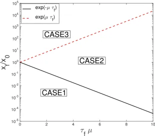
system underx→ −xguarantees exactly equivalent results for x0 <0. Eq. (39) reveals the
following three different cases depending on the sign of γ and the ratio of xf tox0:
• CASE1: γ > e6µτf (x
f < e−µτfx0); • CASE2: γ <0 (e−µτfx
0 < xf < eµτfx0); • CASE3: 0< γ < e6µτf (x
f > eµτfx0).
When x0 = 0, γ = 1, recovering the case in the previous subsection and thus CASE2
becomes irrelevant. That is, x0 6= 0 leads to the appearance of CASE2. For x0 > 0, a
schematic diagram for the different cases is shown in Fig. 1 where xf is plotted against τf.
From Fig. 1, we observe that a short time behavior is described by CASE1/CASE3 while
a long time behavior is obtained from CASE2. As τf increases from zero, the region for
CASE1/CASE3 gradually decreases while the region for CASE2 increases. The cross-over
between CASE1 and CASE2 is set by xf = x0e−µτf ≡ xc while the cross-over between
CASE2 and CASE3 is set by xf =x0eµτf ≡ xd. Here, xc =x0e−µτf is the characteristic of
the movement of the PDF peak. Consequently, the left side of the PDF peak is described
by CASE1 while the right side of the PDF peak by CASE2. On the other hand,xf =x0eµτf
characterises the boundary around which the PDF becomes negligible as Sef f becomes very
large (details not shown here). That is, xb ≡x0e+µτf sets the boundary between the region
of a small probability due to a stochastic noise and a dead zone. (That is, the probability
is zero for xf > xb in CASE3.) To appreciate the meaning of γ, we rewrite
γ = x
3
b −x3f
x3
c −x3f
≡ ∆b
∆c
τ
f
µ
0 2 4 6 8 10
x
f/x
010-5 10-4 10-3 10-2 10-1 100 101 102 103 104 105
exp(-µτ
f)
exp(µ τ
f)
CASE2
CASE3
[image:15.595.137.448.87.359.2]CASE1
FIG. 1: A schematic diagram of xf/x0 againstµτf.
where ∆c =xf −xc and ∆b =xf −xb . Since ∆c and ∆b measure the deviation of xf from
xc and xb, respectively, the probability becomes larger for smaller ∆c and larger ∆b. For
instance, CASE1 with the large value of γ corresponds to the region where the probability
is largest.
To determine the relation between tf and τf along xf =x0e−µτf, we note that Eq. (39)
gives α = x3
0 and B = 0. Thus, the saddle-point solution in Eq. (38) is simplified as
x=x0e−µτ, leading to tf in Eq. (25)
tf =
Z τf
0
dτ1
1 [x(τ1)]2
= 1
2µx2 0
e2µτf −1= 1
2µx2 0
x2 0
x2
f
−1
!
,
and consequently
e2µτf = x
2 0
x2
f
= 1 + 2µtfx20. (40)
In the following subsections, γ >0 (CASE1) and γ <0 (CASE2) are separately considered.
1. CASE1: γ ≥0 (α >0, B <0), xf < x0e−µτf
We first find the relation between tf and τf by using Eq. (38) in Eq. (25) for γ >0. To
do this, we let y=e6µτ and note γ −y >0 (since γ−e6µτf >0) to obtain
tf =
1 6µB23
I0, (41)
where
I0 =
Z yf
1
dy y23
1 (γ−y)23
, (42)
and yf = e6µτf. The integral in Eq. (42) can be written in terms of the generalised
two-family inverse hyperbolic sine (e.g. see [35]). On the other hand, Eq. (26) can be shown
as
Sef f =
µB43 3D I1
= µ
6D
n
6µtf|αB| −3|B|
4 3
h
y13(γ−y) 1 3
iyf
1 o
, (43)
where
I1 =
Z yf
1
dy y
1 3
(γ−y)23
. (44)
In the second line in Eq. (43), we used Eq. (41) and the identity (see Appendix G):
I1 =
1 2
n
γI0−3
h
y13(γ−y) 1 3
iyf
1 o
. (45)
Eq. (43) shows that Sef f becomes zero along the characteristics xf = x0e−µτf as B = 0.
Recall that along these characteristics, Eq. (40) holds. This means that the PDF takes its
maximum value along these characteristics. To facilitate the analysis, it is thus useful to
consider the deviation ∆ from the characteristics by letting
xf =x0e−µτf −∆, (46)
where ∆≥0 since xf ≤x0e−µtf. By using Eqs. (24), (39) and (44) in Eq. (43), we obtain
Sef f =
µ 2D|B|
2µtf(x30+|B|)− xfe3µτf −x0
= µ
2D|B|
2µtf|B|+ ∆e3µτf
, (47)
where α =x3
0 +|B| (as B < 0), h
y13(γ−y) 1 3
iyf
1 = (xfe
3µτf −x
0)|B|−
1
3, and y
f = e6µτf are
used. To obtain the PDF in terms of ∆, we rewrite |B| by using Eq. (46) and Q = y
1 3
e2µτf = 1 + 2µt
fx20 as
|B| = 1
2µtf
3∆Q12 −3∆ 2
x0Q+
∆3
x2 0Q
3 2
Q2+Q+ 1 . (48)
Then, by using Eq. (48) together with Q= 1 + 2µtfx20 from Eq. (40) in Eq. (46), we obtain
the leading order behavior of Sef f in the short and long time limits depending on the value
of Q, respectively, as follows:
Sef f =
∆2
4Dtf
2−3∆
x0
+ 2∆
2
x2 0
, (for Q→1) (49)
∼ µ∆
2
2D
h
∆2(1−1.5Q−1)−3x0∆Q−
1 2 + 3x2
0Q−1 i
. (for Q≫1) (50)
The cross-over between Eqs. (49) and (50) is set by the time whereeµτf ∼1, or equivalently,
tf ≪ (2µx20)−1, independently of D. In the short time limit (Q → 1), the first term in
Eq. (49) demonstrates the Gaussian PDF, the width increasing as t1/2 for small ∆. As
the width broadens, the cubic and quartic terms in ∆ becomes important for the PDF.
In particular, the quartic term leads to the broadening of the PDF width just before the
transition to the second stage governed by Eq. (50) for a sufficiently large time Q≫1.
Notably, Eq. (50) reveals the mixture of the Gaussian PDF, cubic and and quartic
exponential PDF depending on the relative size of the three terms on the right-hand side.
Since x2
0Q−1 ∼ hx2i, we recognise that 3µx20Q−1 = 3µhx2i =µo is the effective linear force
coefficient for fluctuations defined in Eq. (10). Therefore, the third term on the right of
Eq. (50) gives rise to a Gaussian PDF with the inverse temperature∝µo/2D(equivalently,
with the width ∝ p2D/µo). This is remarkably similar to the quasi-linear result and t1/2
increase in the PDF is caused by the decrease in µo as the mean value hxi decreases with
the movement of the PDF peak towardsx= 0.
In comparison, the first term on the right of Eq. (50) leads to a quartic exponential PDF
with the width ∝(2D/µ)1/4 for larger time Q−1 → 0. To compare the size of the first and
third term on the right of Eq. (50), we approximateQ−1 ∼2µx
0tf and ∆ ∼2Dtf to obtain
the estimate of the ratio of the third to the first terms as
3x2 0Q−1
∆2(1−Q−1) ∼
3 4t2
fDµ
Thus, for tf ≪
p
3/4Dµ, the PDF is Gaussian while in the opposite large time, the
PDF relaxes to the quartic exponential PDF. This transition time from the Gaussian to
stationary quartic exponential PDF depends on D, increasing as D becomes smaller.
Finally, it is interesting to observe that in both Eqs. (49) and (50), the first order
correction term has a negative sign (since ∆>0), leading to the increase in the PDF above
the leading order term. This is to be contrasted to CASE2 considered in the next subsection
where the first order correction ∆ is shown to depress the PDF (as Sef f increases).
2. CASE2: γ <0 (α >0, B >0), x0e−µτf < xf < x0eµτf
We begin by rewriting Eq. (38) as
x = B13e−µτ[e6µτ +|γ|] 1
3, (51)
where B (>0) is given by Eq. (24). I0 in Eq. (41) is given by
I0 =
Z yf
1
dy y23
1 (y+|γ|)23
, (52)
where y=e6µt and y
f =e6µτf. Similarly, Eq. (26) can be written as
Sef f =
µB43 3D I1
= µ
2D
n
−2µtf|αB|+B
4 3
h
y13(y+|γ|) 1 3
iyf
1 o
, (53)
where
I1 =
Z yf
1
dy y
1 3
(y+|γ|)23
= 1
2
n
−|γ|I0+ 3 h
y13(y+|γ|) 1 3
iyf
1 o
. (54)
Asxf > x0e−µτf in CASE2, we define ∆ to be the deviation from the characteristics according
to
xf =x0e−µτf + ∆, (55)
where ∆≥0. By using Eqs. (24), (39) and (46) in Eq. (53), we obtain
Sef f =
µ
2DB
−2µtf(x30−B) + xfe3µτf −x0
= µ
2D|B|
2µtfB + ∆e3µτf
where α = x3
0 −B (B > 0), h
y1/3(γ−y)13
iyf
1 = (xfe
3µτf −x
0)B−1/3, and yf = e6µτf are
used. To obtain the PDF in terms of ∆, we again express B by using Eq. (56) and
Q=y
1 3
f =e2µτf = 1 + 2µtfx20 as
B = 1
2µtf
3∆Q12 + 3∆ 2
x0Q+
∆3
x2 0Q
3 2
Q2+Q+ 1 . (57)
Then, by using Eq. (57) and Q = 1 + 2µtfx20 in Eq. (56), we obtain the leading order
behavior of Sef f in the short and long time limit as follows:
Sef f =
∆2
4Dtf
2 + 3∆
x0
+ 2∆
2
x2 0
, (forQ→1) (58)
= µ∆
2
2D
h
∆2(1−1.5Q−1) + 3x0∆Q−
1 2 + 3x2
0Q−1 i
. (for Q≫1) (59)
Similarly to Eqs. (49) and (50) in CASE1, the cross-over between Eqs. (58) and (59) is
set by the time where eµτf ∼ 1, or equivalently, t
f ∼(2µx20)−1, independently of D. In the
short time limit (Q→1), Eq. (58) demonstrates the initial Gaussian PDF, which becomes
modified by the quartic term just before the transition to the second stage governed by
Eq. (59). The second stage in Eq. (59) starts with another Gaussian evolution, followed
by the transition from this Gaussian to the final stationary quartic exponential PDF for
tf ≪
p
3/4Dµ in the long time limit. In contrast to CASE1, in both limits, the first order
correction which is odd in ∆>0 is now positive and results in further decrease in the PDF
as ∆ increases.
C. Summary of CASE1 and CASE2
By combining Eqs. (49)-(50) and (58)-(59), we write Sef f on either side of the PDF peak
in terms ofr =xf −e−µτf as
Sef f =
r2
4Dtf
2 + 3 r x0
+ 2r
2
x2 0
, (for Q→1) (60)
= µr
2
2D
h
r2(1−1.5Q−1) + 3rx0Q−
1 2 + 3x2
0Q−1 i
. (forQ≫1) (61)
Overall, starting from a narrow PDF centered about x = x0, the PDF undergoes three
stages. The first is the Gaussian evolution ending with the broadening of the PDF around
the white noise is balanced by the inertia dx/dt, terminating when the effect of nonlinear
force becomes non-negligible, leading to a slight broadening of the PDF. The nonlinear force
shortly gives rise to a coherent force, initiating the second stage of yet another Gaussian
evolution where fluctuation evolves with the effective frictional force asµo ∝µhxi2 governed
by the O-U process. With further increases in time, the PDF finally settles in to the final
stationary quartic exponential PDF in Eq. (61) for tf ≫tc where
tc ∼
r
3
4Dµ. (62)
(See Appendix H for an alternative derivation of Eq. (62).) The critical time tc in Eq. (62)
increases as D decreases, similarly to the case of x0 = 0 given in Eq. (35), demonstrating
that the final relaxation time to a stationary PDF depends on D and µ (and not on x0).
Aforementioned different stages of PDF evolution and the two characteristic transition
times (tf ∼ (2µx20)−1 and Eq. (62)) are confirmed from the exact solutions obtained by
numerical calculations in §3.
The odd terms in r signify the asymmetry of the PDF around its peak, where the PDF
on the left side of the peak is enhanced over that on the right side of the peak. Recalling
that x0 > 0 in our analysis, this illustrates the enhancement of the PDF around x0 = 0 as
the PDF moves towards xf = 0. This asymmetry property is also confirmed by numerical
calculation in §3.
Finally, the peak amplitude of the PDFs is determined by the normalisation N in Eq.
(15), which is determined by R
dxfp(xf, tf;x0,0) = 1. For the Gaussian PDF of the form
p(x, t) =N e−βx2
, the peak amplitude N =pβ/π∝β1/2 while the width is proportional to
β−1/2. Thus, for the Gaussian PDFs in Eqs. (61)-(62), the behavior of the peak amplitude
of the PDFs can easily be inferred from the effective inverse temperature β. This is
discussed in Section III together with the interpretation of the numerical results. For the
quartic PDF of the form p(x, t) = N e−βx4
III. EXACT PDFS FROM THE FOKKER-PLANCK EQUATION
To complement the analytic study in Section II, we compute numerical solutions of the
time-dependent PDFs. While it would have been possible to obtain the marginal PDFp(x, t)
by stochastic simulation of Eqs. (1) or (6), we instead solve the corresponding Fokker-Planck
equations (e.g. [1, 2])
∂p
∂t =d
∂2p
∂x2 +
∂
∂x x
np
, (63)
wheren= 1 for the linear O-U process, andn= 3 for the cubic process. For convenience, we
use d= 2D whereD is defined in Eq. (2). Without loss of generality, we also setµ0 = 1 for
n= 1 and µ= 1 for n= 3 in Eq. (63). The entire equation can always be rescaled to make
this coefficient one, which is convenient numerically to reduce the number of parameters in
the problem.
To solve these equations numerically, we begin by restricting the interval in x to [−1,1],
rather than the original [−∞,∞]. There is again no real loss in generality involved here; by
suitably rescalingx,t, and/ord, any finite interval can always be mapped to [−1,1]. As long
asdand the initial condition are chosen such thatpwould be negligible outside this interval
anyway, then solving Eq. (63) only on [−1,1], and with p= 0 boundary conditions, should
yield results in good agreement with the analytic formulations. The numerical solution
involves second-order accurate finite-differencing in x, using up to M = 4·106 gridpoints.
The time-stepping is also second-order accurate, with step sizes as small as ∆t= 10−7. Both
M and ∆t were varied to ensure accuracy to within at least 0.1%. Especially in the later
stages of the evolution, once an initially narrow peak has started to broaden considerably,
M can also be decreased and ∆t increased, without loss of accuracy.
The initial condition was taken as
p= √ 1
π10−8 exp
h
−(x−0.7) 2
10−8 i
, (64)
that is, a Gaussian with a peak at x0 = 0.7 and a width 1.7·10−4. The question then is
how this initial condition evolves toward the final equilibrated state, eitherp∝exp(−x2/2d)
for the linear process or p ∝ exp(−x4/4d) for the cubic process, with the constant of
pro-portionality in each case fixed by R
pdx = 1 (see Appendix A). For the linear process, an
analytic solution for the entire time-evolution given in Eq. (3) takes the following form
p(x, t) = √1
2πd 1
√
1−κe−2texp
h
− (x−x0e−
t)2
2d(1−κe−2t)
i
10−6 10−4 10−2 100 102 104 100
101 102 103 104
t
(a)
d=10−3
d=10−7
10−6 10−4 10−2 100 102 104 10−4
10−3 10−2 10−1 100
t
(b)
d=10−3
[image:22.595.134.511.91.244.2]d=10−7
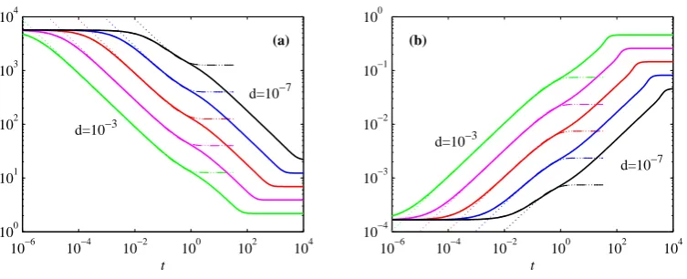
FIG. 2: Panel (a) shows peak amplitudes, panel (b) shows widths at half-peak. In each
panel the heavy solid lines are the cubic case with initial condition (64), the dash-dotted
lines are the linear case with initial condition (64), and the dotted lines are the linear case
with aδ-function initial condition. The five different lines in each set correspond to
d= 10−3 to 10−7, from left to right as indicated.
where κ is an arbitrary constant. Taking κ = 1 would correspond to a δ-function initial
condition, whereasκ= 1−10−8/2d corresponds to the actual initial condition (64).
Fig. 2 shows how the peak amplitudes and widths at half-peak evolve in time, for
the five values d = 10−3 to 10−7. The heavy solid lines show the cubic case that we are
ultimately most interested in. The dash-dotted lines show the linear case with initial
condition (64), and the dotted lines the linear case with a δ-function initial condition
(that is, the dash-dotted lines have κ = 1−10−8/2d in Eq. (65) whereas the dashed lines
have κ = 1). If we first compare the two different initial conditions in the linear case,
we see that a δ-function initial condition relatively quickly (on a timescale ∼ 10−8/d)
becomes indistinguishable from the initial condition (64). This is encouraging, as it
indicates that all the theoretical analysis developed for a δ-function initial condition is still
relevant even for (64). The other point to note about the linear cases is how the
evolu-tion is indeed completed once t ≈ 1, independent of d. Different stages of PDF evolution
with the two transition times above agree with the analytical prediction summarised in§2.3.
101 102 103 104 10−2
10−1
t d=10−3
d=10−7
(a)
101 102 103 104 10−2
10−1
t d=10−3
d=10−7
(b)
101 102 103 104 10−3
10−2 10−1
t d=10−3
d=10−7
[image:23.595.130.508.96.243.2](c)
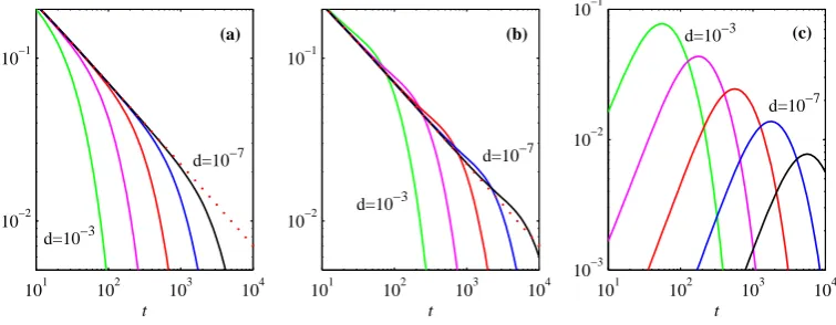
FIG. 3: Panel (a) shows the mean valuehxi, ford = 10−3 to 10−7 as indicated. Panel (b)
showsxpeak, the location wherep takes its maximum value. In both panels the dotted line
denotesx0/ p
1 + 2tx2
0. Panel (c) shows the difference,xpeak− hxi.
linear cases almost exactly. The detailed structure continues to be Gaussian in this regime
(as indicated also by further diagnostics below). For t ≥ O(1) the peaks continue to
decrease and the widths to increase, before eventually settling in to the final equilibrated
solutions where the peaks scale as d−1/4 and the widths as d1/4. Note also how the time
required to reach the final stationary PDF clearly scales as d−1/2, in agreement with the
analytic predictions in §2.3.
Turning next to where p is located, Fig. 3 shows two different ways of measuring this,
the mean value hxi = R
xp dx, and the position of the maximum value of p, call it xpeak.
Up to t ≈ 1 both measures are essentially indistinguishable from the expected result
x0/ p
1 + 2tx2
0 for small fluctuations h(δx)2i ≪ hxi2; as fluctuations increase with time,
deviations do begin to appear as shown in the range t > O(1) in Fig. 3. As predicted in
Eq. (9), hxi tends to zero somewhat faster than expected from x0/ p
1 + 2tx2
0, especially
for the larger values of d. This is due to the contribution from fluctuations h(δx)2i in
Eq. (9) which increases with d. Since larger d corresponds to greater variance, hxi tends
to zero faster. That is, fluctuations lead to the enhanced dissipation of the mean value.
Consideringxpeak next, this ultimately follows the same trend of tending to zero faster, and
with the same variation with d. It is interesting to note that for brief intermediate times
these curves are slightly abovex0/ p
1 + 2tx2
10−1 100 101 102 103 104 −0.6
−0.4 −0.2 0
t d=10−3
d=10−7
(a)
10−1 100 101 102 103 104 2
2.5 3 3.5
t d=10−3
d=10−7
(b)
10−1 100 101 102 103 104 0.3
0.35 0.4 0.45 0.5
t d=10−3
d=10−7
[image:24.595.127.511.95.239.2](c)
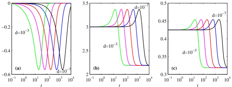
FIG. 4: Panel (a) shows the skewness R
((x− hxi)2/σ)3p dx, panel (b) shows the kurtosis
R
((x− hxi)2/σ)4p dx, and panel (c) the ratio of variance to half-peak width. In each panel
d varies from left to right as 10−3 to 10−7. Note the ∝d−1/2 scaling in time.
between these two measures of position. For all five values of d there are times where this
difference is surprisingly large, comparable to the larger of the two at the corresponding time.
The fact that these two measures of location give somewhat different answers is already
indicative of the result noted above, that the PDF is expected to be asymmetric about
its peak. This can be further quantified by computing the skewness R
((x− hxi)2/σ)3p dx,
where σ= [R
(x− hxi)2p dx]1/2 is the variance. Another interesting quantity is the kurtosis
R
((x− hxi)2/σ)4p dx. Analytically one finds easily enough that a Gaussian profile has
kurtosis 3, whereas the final quartic profile has kurtosis 2.19 (e.g. see Appendix A). A third
quantity to consider is the ratio of the varianceσ to the half-peak width. For this one finds
analytically that a Gaussian has 0.425, whereas a quartic has 0.319. Fig. 4 shows how
these three diagnostics evolve in time. The skewness starts and ends at zero, as expected,
but at intermediate times reaches a peak negative value of -0.56, reflecting this difference in
the two location measures in Fig. 3. This negative value of skewness is predicted in §2.3.
The kurtosis similarly starts at 3 and ends at 2.19, as expected, but at intermediate times
actually increases to a peak of 3.37. The variance/width ratio follows the same pattern as
the kurtosis.
the stationary PDF is very different from the non-equilibrium PDF. Second, the broadening
of the PDF in the intermediate time before reaching the stationary PDF is reminiscent of a
cyclic geodesic solution in [18], suggesting an important role of nonlinear interaction (force)
in a geodesic. Detailed discussion on the implications of these results for information change
is provided in [38]. The last point to note about all three diagnostics is how the curves for
different values of d are essentially identical, but offset in time according to a d−1/2 scaling.
This is another reflection of the result derived analytically and discussed in Section II.C
(see. Eq. (62)) and also seen in Fig. 2 that the final adjustment timescale for the cubic
process scales as d−1/2.
IV. CONCLUSION
We have presented time-dependent PDFs in a cubic nonlinear stochastic process where
the frictional force is given by a cubic nonlinearity. Analytically, we applied an instanton
method based on a path integral formulation to a nonlinear system in the limit of weak noise
(small D) and proposed a new nonlinear time transformation to solve nonlinear instanton
(saddle-point) equations. We predicted a PDF which is in general given as an integral and
elucidated the effect of nonlinear interaction on enhanced dissipation in relaxation processes.
Useful local time-dependent PDFs were presented in certain limits (e.g. in the short and
long time limits). In sharp contrast to a linear stochastic process where transient PDFs
are Gaussian and the relaxation time tf to the final stationary PDF is independent of the
diffusion coefficient D, the PDF in the cubic process was shown to be asymmetric around
its peak while the relaxation time tf > tc ∼ √µD1 in Eq. (62) depends on D, increasing as
D decreases. The latter reflects a close interlinking between space and time in nonlinear
relaxation processes. Alternatively, time flows at a different rate depending on the
coordi-nate. We also demonstrated the utility of generalised two-family trigonometric functions in
solving nonlinear equations. Numerical simulation of the Fokker-Planck equation revealed
detailed evolution of the time-dependent PDF; analytical and numerical results agreed on
overall PDF evolution, in particular, transition times for different evolutions (e.g. relaxation
timetf) and asymmetry, as noted in§2.3 and§3. Furthermore, it highlighted that transient
PDFs behave drastically differently from the stationary PDFs in regards to the asymmetry
nar-row stationary PDF only after undergoing a transient state with asymmetric and broad PDF.
The generality of our methodology and predicted exponential PDF are reminiscent of
the possibility of transforming any automonous nonlinear Langevin equation driven by a
white noise to the Brownian motion, while our new proposed nonlinear time transformation
plays a role of random time change – the so-called Lamperti transformation [2, 3]. The latter
transforms away a nonlinear diffusion coefficient (D) to a constant diffusion (e.g. see [36, 37]
and Theorems 7.37 and 7.39 and Remark 7.4, Chap 7 in [2]). Together with the change of
variables, or change of measure (Girsanov transformation) which removes the drift term (i.e.
∂V
∂x in our case), the solution to any stochastic equation with time-independent coefficient can
be obtained by the Brownian motion (e.g. see [2, 3]). However, since the resulting Brownian
motion depends on random time, it is not clear how to calculate transient PDFs by using this
method. In comparison, our nonlinear time transformation seems to offer a systematic way of
computing the PDFs in different limits. This opens a large scope for future study including
the application of our method to other nonlinear stochastic processes. Of particular interest
would be the inclusion of a linear (negative) force in the cubic process to investigate the
dynamics of growth, phase transition and long-term memory. A change of variables would
then permit us to examine the Feller-branching process with a logistic growth (e.g. see [36]).
Furthermore, the investigation of the change in information in nonlinear processes in terms
of information length [17] is addressed in the accompanying paper [38].
Appendix A: Property of p(x) =Nexp(−βx4).
We first show how to fix N by the unity of the total probabilityR∞
−∞dx p(x) = 1:
N−1 =
Z ∞
−∞
dx e−βx4
= 2
Z ∞
0
dx e−βx4
= 1
2β
−1 4
Z ∞
0
dy y−34e−y
= 1
2β
−1 4Γ
1 4
where the change of the variable y = βx4 (dx = 1 4β−
1 4y−
3
4dy) was used and Γ(z) =
R∞ 0 dy y
z−1e−y is the Gamma function. That is,
p(x) = 2β
1 4 Γ 1 4 e− βx4 .
By using Eq. (A1), we can calculate the second and fourth moments as follows:
hx2i =
Z ∞
−∞
dx x2p(x) = 2N
Z ∞
0
dx x2e−βx4
= N
2β
−1 4β−
1 2
Z ∞
0
dy y−14e−y
= Γ 3 4 Γ 1 4 β− 1
2, (A2)
and
hx4i =
Z ∞
−∞
dx x4p(x) = 2N
Z ∞
0
dx x4e−βx4
= N
2β
−1 4β−1
Z ∞
0
dy y14e−y
= Γ
5 4
Γ 14β− 1 = 1
4β
−1, (A3)
where Γ(z) = (z−1)Γ(z) was used for z = 5
4 in the last line.
From Eq. (A2) and Eq. (A3), we find the kurtosis κ:
κ = hx
4i
hx2i2 =
1 4
Γ 14
Γ 34 !2
= 2.1884. (A4)
Thus, the quartic exponential PDF has kurtosis less than 3, indicating narrow width and
flatness. Note that the Gaussian PDF has κ= 3.
Appendix B: Path integral in Eq. (12)
For Gaussian statistics with vanishing first moment, the prescription of the second
mo-ment given by Eq. (2) is sufficient. It is simply because all odd momo-ments vanish while even
moments can be expressed as a product of second moments. Note that even if the forcing is
equation. An equivalent way of prescribing the second moment (2) for the Gaussian forcing
is to introduce the probability density function for ξ as follows [12, 26, 33]
d[ρ(ξ)] = Dξexp
−12
Z
dtD−1ξ(t)2
. (B1)
This is a Gaussian distribution forξ(t). The average value of a quantityQis then computed
as
hQi=
Z
d[ρ(ξ)]Q .
For instance, by taking Q=ξ(t)ξ(t′), one can easily reproduce Eq. (2).
When the average value of a functional ofx(i.e. hQ[x]i) is required, the constraint should
be imposed that ξ and x satisfy the original equation (1). This can be done by inserting an
identity with aδ-function, which enforces Eq. (1), as
1 =
Z Dx δ
dx
dt +
∂V
∂x −ξ
J
∝ Z
DxDx exp
i Z dt x dx dt + ∂V
∂x −ξ
ψ, (B2)
where J =J∂ξ
∂x
is the Jacobian due to the change of variables for the delta function. Let
us show in detail how this is done. Starting from the definition,
hQ[x]i =
Z
Dξ Q[x] exp
−2D1
Z
dtξ(t)2
=
Z
DξDx Q[x]δ
dx
dt +
∂V
∂x −ξ
J
×exp
−2D1
Z
dtξ(t)2
=
Z
DξDxDx Q[x] exp
i Z dt x dx dt + ∂V
∂x −ξ
J
×exp{− 1 2D
Z
dtξ(t)2}
=
Z
DxDx Q[x]e−S. (B3)
Here, we used the identity Eq. (B2) to obtain the second line andJ =e−ψ and ψ =−3
2µx 2
(see, e.g. Eq. (96)-(97) in [33], Eq. (2.10) in [12]) for V(x) = µx4/4 to obtain the last
line. the Gaussian integral over ξwas performed to obtain the last line of Eq. (B3); S is the
action given in Eq. (12) in the main text. TakingQ[x] =δ(x(tf) =xf)δ(x(0) =x0) gives us
Eq. (11) in the text. Note thatx is a conjugate variable, which acts as a mediator between
Appendix C: Nonlinear transformation Eq. (18)
Let us consider a homogeneous cubic equation dx
dt =−µx
3. The usual way of solving this
equation is to separate variables and integrate to obtain
x(t) = p x0
1 + 2µtx2 0
, (C1)
where the initial condition x(t = 0) = x0 is used. To elucidate how the nonlinear
transfor-mation defined in Eq. (18) works, we rewrite dx
dt =−µx
3 as follows:
0 = dx
dt +µx
3 =x2(dx
dτ +µx). (C2)
The solution to Eq. (C2) is x(τ) = x0e−µτ wherex0 =x(τ = 0) =x(t= 0). To obtain x(t),
we use x(τ1) =x0e−µτ1 in Eq. (25):
t =
Z τ 0
dτ1
1 (x(τ1))2
= 1
2µx2 0
e2µτ −1
= 1
2µx2 0
x2 0
(x(t))2 −1
. (C3)
Solving Eq. (C3) for x(t) gives the same solution Eq. (C1).
Appendix D: Generalised two family trigonometry functions
The generalised sine function with two parameters p, q, wherep >1 and q >1, is defined
through its inverse function [35]
arcsinp,q(x) =
Z x 0
dt(1−tq)−1/p, (D1)
where x = [0,1]. Note that when p = q = 2, Eq. (D1) recovers the definition of the usual
arcsin(x). Whenx= 1, Eq. (D1) defines the generalised πp,q as
arcsinp,q(1) =
Z 1
0
dt(1−tq)−1/p= πp,q
2 , (D2)
which again recovers π/2 when p = q = 2. We note that sinp,q(x) is a monotonically
increasing function of x, mapping [0,1] → [0, πp,q/2] and Eq. (D1) can also be written in
terms of Gaussian hypergeometric function.
The (p, q)-cosine is defined as
cosp,q(x) =
dsinp,q(x)
dx = (1−(sinp,q(x))
where x is a real number. Hence, cosp,q(x) is strictly decreasing on [0, πp,q/2], cosp,q(0) = 1,
cosp,q(πp,q/2) = 0 and satisfies the following identity:
|sinp,q(x)|q+|cosp,q(x)|p = 1, (D4)
which is Eq. (29) with x=zf.
Appendix E: Derivation of Eq. (32)
To show the identity Eq. (32), we let the left-hand side of Eq. (32) be I1 and re-express
it as follows:
I1 ≡
Z z 0
dz1
1 (1−z3
1)5/3
(E1) = Z z 0 dz1
1−z3 1
(1−z3 1)5/3
+ z
3 1
(1−z3 1)5/3
(E2)
≡ I0+ Z z
0
d[(1−z13)−2/3]z1
2 (E3)
= I0+
1 2
z
(1−z3)2/3 −
1 2 Z z 0 dz1 1 (1−z3
1)2/3
(E4)
= I0+
1 2
z
(1−z3)2/3 −
1 2I0 =
1 2I0+
1 2
z
(1−z3)2/3 (E5)
= 1
2
Z z 0
dz1(1−z13)−2/3+z(1−z3)−2/3
, (E6)
obtaining Eq. (32) in the text. Here,I0 in Eqs. (E3)–(E5) is defined as
I0 ≡
Z z 0
dz1
1 (1−z3
1)2/3
, (E7)
and integration by parts is used to obtain Eq. (E4) from Eq. (E3).
Appendix F: For y−γ >0
In this case, we obtain from Eq. (38) and Eq. (25)
t = 1
6µB23
I0, (F1)
where
I0 =
Z yf
1
dy y23
1 (y−γ)23
Here, y =e6µt and y
f =e6µτf. Similarly, Eq. (38) can be written as
Sef f =
µB43 3D I1
= µ
6D
n
6µtf|αB|+ 3B
4 3
h
y1/3(y−γ)13
iyf
1 o
, (F3)
I1 =
Z yf
1
dy y
1 3
(y−γ)23
. (F4)
In the second line in Eq. (F3), we used Eq. (F1) and the following identity (similar to
that used in Appendix C):
I1 =
1 2
n
γI0+ 3 h
y1/3(y−γ)13
iyf
1 o
. (F5)
Appendix G: Derivation of Eq. (45)
We rewrite I0 in Eq. (42) in terms of I1 in Eq. (44) as
I0 =
Z yf
1
dy y−
2 3
(γ−y)23
= 1
γ [I1+J], (G1)
where
J =
Z yf
1
dyy−23(γ−y) 1 3
= 3
h
y13(γ −y) 1 3
iyf
1 +
1 3
Z yf
1
dyy13(γ−y)− 2 3
= 3hy13(γ−y) 1 3
iyf
1 +I1. (G2)
By using Eq. (G2) in Eq. (C1), we obtain
γI0 = 2I1+ 3
h
y13(y−γ) 1 3
iyf
1 ,
which gives Eq. (45).
Appendix H: Alternative derivation of the relaxation time to the stationary PDF
To estimate the relaxation time to the stationary PDF, we let r =r(0)+r(1) in Eq. (61)
by assuming a small Q−1 and find
By comparing the two terms in r above, we conclude that the critical time tc required to
relax into the equilibrium PDF satisfies
tf >
9
32√2Dµ (≡tc). (H1)
[1] H. Risken, “The Fokker-Planck Equation: Methods Of Solution And Applications: Methods
of Solutions and Applications”, 3rd Ed. Springer (2013).
[2] C. Klebaner, “Introduction to Stochastic Calculus with Applications”, Chap. 5.5, Imperial
College Press (2012).
[3] C. Gardiner, “Stochastic methods”, 4th Ed., Springer, Chap. 4.4. (2008).
[4] H. Haken, “Information and Self-organization: A macroscopic approach to complex systems”,
3rd Ed., Springer, p.63-64 (2006).
[5] B. R´enyi, Proceedings of the fourth Berkeley Symposium on Mathematical Statistics and
Probability, 547 (1960).
[6] A. D. Wissner-Gross and C. E. Freer, Phys. Rev. Lett. 110, 168702 (2013).
[7] A. Caticha, AIP Conf. Proc. 617, 302 (2001).
[8] D. Acosta, F. F. de C´ordoba, J.M. Isidro, and J.L.G. Santander, arXiv1107.1898A (2011).
[9] S.-I. Itoh, K. Itoh, M. Yagi, M. Kawasaki, and A. Kitazawa, Phys. Plasmas9, 1947 (2002).
[10] C. Tsallis, “Introduction to nonextensive statistical mechanics : approaching a complex
world”, Springer (2009).
[11] S.P. Das and G.F. Mazenko, J. Statistical Phys.149, 643 (2012).
[12] P. H¨anggi, Z. Phys. B – Condensed Matter 75, 275 (1989).
[13] J. Anderson and E. Kim, Plasmas Phys. Control. Fusion52, 012001 (2010).
[14] E. Kim, H. Liu and J. Anderson, Phys. Plasmas16. 0552304 (2009).
[15] E. Kim and P.H. Diamond, Phys. Rev. Lett. 88, 225002 (2002).
[16] E. Kim and P.H. Diamond, Phys. Plasmas9, 71 (2002).
[17] J. Heseltine and E. Kim, J. Phys. A: Theo. & Math. 49, 175002 (2016).
[18] E. Kim, U. Lee, J. Heseltine and R. Hollerbach, Phys. Rev. E. 93, 062127 (2016).
[19] S.B. Nicholson and E. Kim, Phys. Lett. A. 379, 8388 (2015).
[21] E. Kim and S. Nicholson, Phys. Lett. A 379, 1613 (2015).
[22] R. Hermann, “Fractional Calculus: An Introduction for Physicists”, World Scientific (2011).
[23] J. Anderson, E. Kim and S. Moradi, Phys. Plasmas21, 122109 (2014).
[24] M.H. Pinsonneault, S. D. Kawaler, S. Sofia, and P. Demarque, Astrophys. J.338, 424 (1989).
[25] E.T. Lu, Phys. Rev. Lett.74, 2511 (1995).
[26] J. Zinn-Justin, “Quantum Field Theory and Critical Phenomena”, Chaps. 2-4, Oxford Science
Publications (2008).
[27] J. Zinn-Justin and U.D. Jentschura, Ann. Phys.313, 197 (2004); 269 (2004).
[28] U.D. Jentschura and J. Zinn-Justin, Ann. Phys.326, 218 (2011).
[29] U.D. Jentschura, A. Surzhykov and J. Zinn-Justin, Ann. Phys.325, 1135 (2010).
[30] R.P Feynman and A.R. Hibbs, “Quantum Mechanics and Path Integral”, Chap. 2,
McGraw-Hill Book Company (1965); R.P. Feynman, “Statistical Mechanics”, Chap. 3, W.A. Benjamin,
Inc (1972).
[31] G. ‘t Hooft, Phys. Rev. Lett.37, 8 (1976).
[32] V. Gurarie and A. Migdal, Phys. Rev. E 54, 4908 (1996); G. Falkovich, et al., Phys. Rev. E
54, 4896 (1996).
[33] U. Seifert, Stochastic Thermodynamics, Soft Matter, From Synthetic to Biological Materials,
39th IFF Spring School, (2008).
[34] E. Hopf, Comm. Pure Appl. Math.3201 (1950); P. Lagestrom, J.D. Cole and L. Trilling,
Prob-lems in the theory of viscous compressible fluids, California Institute of Technology (1949).
[35] D.E. Edmunds, P. Gurka and J. Lang, J. Math. Anal. Appl.420, 16801692 (2014); L. Boulton
and G.J. Lord, Proc. R. Soc. A471, 20140642 (2016); B. A. Bhayo and M. Vuorinen, Journal
of Approximation Theory 164, 14151426 (2012).
[36] A. Lambert, Ann. Appl. Prob.15, 1506 (2005).
[37] L.E. Dubins and G. Schwarz, Proc. Nat. Acad. Sci.53, 913 (1965).
[38] E. Kim and R. Hollerbach, “Signature of fractal geometric structure in non-equilibrium