Longevity Basis Risk A methodology for assessing basis risk

City, University of London Institutional Repository

Citation

:

Millossovich, P., Haberman, S., Kaishev, V. K., Baxter, S., Gaches, A.,

Gunnlaugsson, S. and Sison, M. (2014). Longevity Basis Risk A methodology for assessing

basis risk. Institute and Faculty of Actuaries (IFA) , Life and Longevity Markets Association

(LLMA).

This is the published version of the paper.

This version of the publication may differ from the final published

version.

Permanent repository link:

http://openaccess.city.ac.uk/16835/

Link to published version

:

Copyright and reuse:

City Research Online aims to make research

outputs of City, University of London available to a wider audience.

Copyright and Moral Rights remain with the author(s) and/or copyright

holders. URLs from City Research Online may be freely distributed and

linked to.

City Research Online: http://openaccess.city.ac.uk/ [email protected]

Longevity Basis Risk

A methodology for assessing basis risk

by Cass Business School and Hymans Robertson LLP

Research Report

Longevity Basis Risk

A Methodology for Assessing Basis Risk

Research investigation and report by Cass Business School and

Hymans Robertson LLP for the Institute and Faculty of Actuaries and the

Life and Longevity Markets Association

Written by

Prof Steven Haberman FIA, Prof Vladimir Kaishev, Dr Pietro Millossovich,

Andrés Villegas MACA

For and on behalf of Cass Business School

Steven Baxter FIA, Andrew Gaches FIA, Sveinn Gunnlaugsson GradStat,

Mario Sison

For and on behalf of Hymans Robertson LLP

December 2014

Introduction

On behalf of the joint Longevity Basis Risk Working Group (LBRWG) established by the Life and Longevity Markets Association (LLMA) and the Institute and Faculty of Actuaries (IFoA), I am delighted to introduce the results of this research project.

This technical report details the methodology developed on behalf of the LBRWG to assess longevity basis risk. A user-guide which provides a high level summary of this report has also been produced. Together these documents form the key outputs of the first phase of a longevity basis risk project commissioned and funded by the IFoA and the LLMA, and undertaken on our behalf by Cass Business School and Hymans Robertson LLP.

The importance of longevity basis risk

Longevity basis risk arises because different populations, or subpopulations, will inevitably experience different longevity outcomes. This is a significant issue for those wishing to hedge longevity risk using a published mortality index – whether they be pension schemes, insurers, reinsurers or banks. To put it simply, actual longevity outcomes, and therefore cashflows, of the hedged portfolio will differ from those under the hedging instrument.

In addition, longevity basis risk can also present a wider issue for insurers using, in their reserving models, external data, such as population data, rather than their own policy data. The need to quantify and reserve for any potential basis risk is receiving increasing focus, particularly under Solvency II.

Demographic aspects of longevity basis risk

There are several aspects of longevity basis risk. This research focuses on the impact of

demographic and socio-economic differences between the portfolio and the index population, which can lead to different initial rates and trends in mortality. To date, there has been no well-established methodology for assessing these demographic aspects of longevity basis risk.

Historical differences demonstrate the need to assess basis risk

A review of existing literature and analysis of pension scheme data have provided evidence that historic mortality improvement rates have varied by socio-economic class and deprivation. These variations have been significant and sometimes as large as the variation by gender. This

of the portfolio being hedged. Given this model, the assessment of other aspects of basis risk, such as sampling risk and structuring risk, becomes (in theory, at least) more straightforward.

Delivering a framework to assess longevity basis risk

I am delighted that the research has delivered a framework for assessing longevity basis risk. This recognises the fact that different users, with different portfolios, will have different constraints on the models they can use in practice. The research has identified specific models and techniques for different situations, which we believe will provide a good starting point for assessing basis risk.

We are delighted to be able to present this research and hope it will prove of value to practitioners and enable an important step change in the ability to assess longevity basis risk.

Pretty Sagoo

Chair of the LLMA and IFoA Joint Longevity Basis Risk Working Group

Scope, reliances and limitations

This report has been produced by Hymans Robertson LLP and Cass Business School for the Longevity Basis Risk Working Group (LBRWG) of the Institute & Faculty of Actuaries (IFoA) and the Life and Longevity Markets Association (LLMA).

The scope of this phase of work is limited to producing a proposed methodology for assessing (demographic) basis risk. For

example identification and development of appropriate metrics for assessing basis risk, quantification of potential capital

savings and presentation of basis risk results to regulatory authorities are excluded from this initial phase and (potentially) form part of a secondary phase of this project.

This report is addressed to the LBRWG. It may be shared with members of the IFoA and LLMA and other relevant third

parties. This report does not constitute advice and should not be considered a substitute for specific advice in relation to individual circumstances. While care has been taken to ensure that it is accurate, up to date and useful, neither Hymans

Robertson LLP, Cass Business School, the IFoA nor the LLMA accept liability for actions taken by third parties as a

Executive Summary

This paper summarises the work to date of Cass Business School and Hymans Robertson LLP in relation to assessing longevity basis risk. This work was commissioned by the Longevity Basis Risk Working Group (LBRWG) and funded by the Life and Longevity Markets Association (LLMA) and Institute and Faculty of Actuaries (IFoA). The LBRWG was formed by the LLMA and IFoA in December 2011 with a remit to investigate how to provide a market-friendly means of analysing longevity basis risk.

The key outputs of this work are:

 for modelling books which are ‘self-credible’ (i.e. a large number of lives & sufficient back history) a shortlist of ‘best of breed’ 2 –population models (specifically the M7-M5 model, or in some situations the CAE+Cohorts model);

 for modelling the majority of books which are not self-credible, an alternative, easy to apply “characterisation approach”;

 a clear decision tree framework to aid the selection of an appropriate methodology for assessing basis risk from those mentioned above;

 a clear recognition of the importance of choice of time series underpinning any 2- (or multi-) population model

These outputs are backed up by an extensive body of research, including:

 a review of how trends have varied between different (sub) populations in the past, covering both the highlights of existing literature and additional research based on the Club Vita dataset of UK occupational pension schemes;

 a review, classification and general formulation of two-population models that could be considered for modelling longevity basis risk;

 a thorough and systematic assessment of candidate two-population mortality models to identify those which provide the most suitable balance between flexibility, simplicity, parsimony, goodness-of-fit to data and robustness;

 case studies, review of key challenges and consideration of practicalissues in relation to both the M7-M5 model and the characterisation approach.

Introduction to longevity basis risk

When insurance companies and pension schemes consider managing their longevity risk one of the available options is to use a hedging instrument based upon published mortality indices. However this has a risk that the actual longevity outcomes (and so cashflows) of the hedged portfolio may differ from those under the hedging instrument.

Historical differences in mortality improvement rates demonstrate the need to assess basis risk

Our review of existing literature demonstrates clearly that mortality improvement rates have historically varied by socio-economic class and deprivation. These variations have been significant – indeed they have been as large as the variation seen by gender. This conclusion is confirmed by analysis of the trends in the Club Vita dataset of occupational pension schemes.

The size of these variations demonstrates the significance of demographic basis risk and confirms the need to model longevity basis risk.

The need for a two-population model

In order to be able to assess basis risk, we need a model that is able to capture the mortality trends in the reference population backing the hedging instrument and in the book population, the longevity risk of which is to be hedged. This modelling is needed in order to generate a distribution of future scenarios to evaluate the possibly different evolution of mortality in the two populations. Given this model, the assessment of sampling risk and structuring risk becomes (in theory, at least) straightforward.

Directly modelling basis risk

If a book is ‘self-credible’ (i.e. has large number of lives and sufficient back history) it is possible to parameterise a two-population model directly from mortality experience data relating to i) the population underlying the index and ii) the book population.

Our systematic assessment of candidate two-population mortality models identified two particular ‘best of breed’ two–population models (specifically the M7-M5 model, or in some situations the CAE+Cohorts model).

Parametric form for shape of mortality with age (‘M7-M5’)

The M7-M5 model is a two-population extension of the Cairns-Blake-Dowd (CBD) model of mortality introduced in Cairns, Blake, & Dowd (2006).

Readers may be familiar with the Cairns-Blake-Dowd family whereby the logit of mortality (as measured by 𝑞𝑥)

takes up to a quadratic form with age. Within this family of models we find incorporating both a quadratic term (to capture shape sensitivities at older ages) and a cohort term leads to the best performance for the reference population, and results in the model often referred to as ‘M7’ as per Cairns et al (2009):

Thus the (M7) model for the reference population R takes the form:

logit 𝑞𝑥𝑡𝑅 = 𝜅𝑡(1,R)+ (𝑥 − 𝑥̅)𝜅𝑡(2,R)+ ((𝑥 − 𝑥̅)2− 𝜎𝑥2)𝜅𝑡(3,R)+ 𝛾𝑡−𝑥𝑅

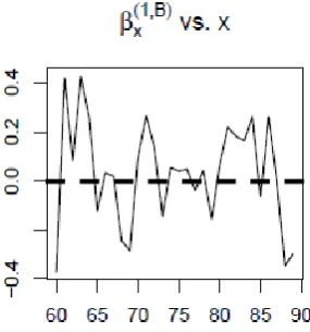
The difference between book population B and reference population R takes the form of a simplified Cairns-Blake-Dowd model, with linear age sensitivity and no cohort effect, often referred to as ‘M5’.

Hence the (M5) model for the difference between book population B and reference population R takes the form:

logit qBxt− logit qxtR = κt(1,B)+ (x − x̅)κt(2,B)

Non-parametric form for shape of mortality with age (‘CAE+cohorts’)

If we instead allow the shape of mortality to have a non-parametric relationship with age we obtain the extended Lee-Carter family of models. Within these models we find a Lee-Carter model with the addition of a cohort term performs best for the reference population

Thus the (Lee-Carter with cohort term) model for reference population R takes the form:

The difference between book population B and reference population R takes the form

logit qxtB − logit qxtR = αxB+ βxRκtB

This model is referred to as the common age effect as the book population has a Lee-Carter form with the same sensitivity by age to time based improvements as the reference population.

Indirectly modelling basis risk – Characterisation approach

If the book is not ‘self-credible’, (i.e. it does not have a sufficiently large number of lives or lacks a sufficient back history) then it is not possible to robustly parameterise the book element of a two-population model directly from mortality experience data. In this situation an alternative approach is required.

Indeed, even where the book is sufficiently large with long enough experience history to use direct modelling, an alternative indirect approach may still be useful; either as a means of a pragmatic initial assessment of the quantum of basis risk, or as an alternative approach as part of considering model risk.

The alternative we propose, which we describe as a “characterisation approach” enables an assessment of basis risk based on the characteristics of the book in question; leveraging an alternative larger dataset to provide the required volumes and back history of data.

Instead of using the experience data of the book itself, the basic principle of the characterisation approach is to map the book onto a small number of characterising groups which:

 capture the majority of the source of demographic risk

 can be projected using an alternative data source with a more reliable and longer back-history of mortality experience

Schematically, this approach can be thought of as:

In the schematic above, the book population 𝐵 is subdivided into three distinct subgroups 𝐵1, 𝐵2 and 𝐵3,

according to some characterising criteria. Both 𝐵 and the subpopulations 𝐵1, 𝐵2 and 𝐵3 are too small for direct

modelling. However, a larger characterising population 𝐶 is available, and has previously been segmented (using the same characterising criteria) into subgroups 𝐶1, 𝐶2 and 𝐶3. Importantly, 𝐶 has been chosen such that

It is now possible to simulate 𝐵 indirectly, by first simulating 𝐶1, 𝐶2 and 𝐶3and mapping those simulations across

to 𝐵1, 𝐵2 and 𝐵3.

Choosing between approaches

A flow chart (see next page) has been developed to assist users (based on their requirements) in choosing between direct modelling and the characterisation approach. In addition, it provides assistance in choosing between M7-M5 and CAE+Cohorts models where direct modelling is preferred.

Having assessed direct modelling under M7-M5 and CAE+Cohorts models for book populations of different size and history length, a key requirement for direct modelling (reflected in the first question) is sufficient data; typically over 25,000 lives and in excess of 8 years history.

In addition direct modelling relies on the assumption that “past data is a good guide to the future”. This may not always be the case, hence the second question relating to whether there have been any major changes in the socio-economic mix in the book over time.

There are a number of considerations which could be taken into account in choosing between M7-M5 and CAE+Cohorts (including user familiarity or preference), but a specific practical issue, relating to the typical need to allow for inter-age mortality correlations is covered by the third question.

Finally, in some cases there could be a strong belief in a book specific cohort effect (which would require an extension to the form of the model for book population); this is covered by question 4.

Case studies, key challenges and practicalities

Case studies are provided for both direct modelling and the characterisation approach. In addition we seek to identify (and suggest approaches to tackle) key challenge and practicalities in the application of these methods.

Sensitivity to choice of model and choice of time series

The alternative methods illustrated (M7-M5 and CAE+Cohorts for direct modelling, and the characterisation approach) provide for the most part similar conclusions on the amounts of basis risk. But differences do exist, illustrating the issue of model risk.

We focus on a number of well-established choices of time series in the models; the alternatives used

demonstrate the model risk associated with choice of time series; a comprehensive exploration of alternatives and their impact is outside the scope of this research project. Nonetheless it is appropriate to flag the risk associated with choice of time series and highlight the benefit that further assessment, development and guidance on the choice of time series would bring to practitioners.

Nature of this paper

C

ontents

Longevity Basis Risk PAGE

Executive Summary 2

1 Introduction 8

2 Observed differences in mortality improvements 12

3 High level review of drivers 23

4 Modelling problem 28

5 Overview of available models 29

6 Identifying an appropriate two population model 35

7 A framework for modelling demographic basis risk 58

8 Case study – Direct modelling 68

9 Key challenges and practicalities of direct modelling 73

10 Characterisation Approach 80

11 Case study – characterisation approach 90

12 Practicalities of characterisation approach 99

References 101

Appendix A: Club Vita data 105

Appendix B: Landscape of two-population models 109

Appendix C: Overview of time series 113

Appendix D: Characterising groups for the Club Vita dataset 115

Appendix E: Generation of synthetic data 121

1

Introduction

1.1 Longevity risk transfer market

Recent years have seen a huge growth in longevity risk transfer, both in the insurer to reinsurer market, and from pension schemes to the insurance market1. An effective, growing market with sufficient capacity to meet demand would be to the benefit of all participants, whether to enable business to be done, or to manage risk.

To date most transactions have been “bespoke” deals, with the payouts linked directly to the actual experience or lifespans of the individuals being covered. But index-based solutions – where the payouts are linked to a longevity index or metric based on an external reference population – are possible. They have the potential to provide important benefits: lower costs, faster execution, potential for liquidity, and greater transparency.

1.2 Enabling the development of index based solutions

Many steps have been taken to enable index-based solutions to develop. Publication of indices by the LLMA, Deutsche Börse and others; continued innovation of possible structures such as the Longevity Experience Options introduced by Deutsche Bank; and papers on standard derivative structures such as q- and S- forwards2.

But one key issue remains – that of “longevity basis risk”. How good a match will there be between a portfolio’s experience, and that reflected by an external, published, longevity index? How much protection can index- based solutions provide?

1.3 The question of longevity basis risk

In its simplest form an index based longevity swap involves a payment to the pension scheme or insurer that is based on the longevity experience of a reference index. An index–based swap provides a means to obtain (partial) protection from longevity risk both for pensioners but also deferred pensioners who are generally not covered by the “bespoke” transactions. In the case of life insurers they offer a potentially flexible way to manage exposure to longevity risk, or to facilitate a more capitally optimal balance between longevity and mortality risk. However index-based swaps do not provide a perfect risk reduction. The index based payments will not exactly match the actual annuity payments being made by the insurer or pension scheme.

Understanding the residual longevity risk and “how good” the risk reduction is, is key. The kinds of practical questions asked about index-based swaps include:

 What is the risk that index payments will fall short of annuity payments?

 How can we determine the “hedge effectiveness”?

 How can we do a cost-benefit analysis of an index-based hedge?

 How do we determine an appropriate capital reduction for an index-based hedge?

To answer these questions, we need a practical and realistic way of modelling and quantifying basis risk.

1

For example in the year to 30 June 2014 £39bn of longevity risk was transferred from pension schemes to insurers and reinsurers via buy-ins, buy-outs and longevity swaps. Of this £27bn related to longevity only transactions (longevity swaps), close to double the volume written in the preceding 4 years. (Hymans Robertson (2014))

2

1.4 Sources of basis risk

There are three primary sources of basis risk3:

1 Structuring risk due to the pay-off of the hedging instruments being different to that of the portfolio (for example the hedging instrument making annual payments whereas the portfolio pays annuities or pensions monthly, or the hedge may be of shorter duration than the liabilities).

2 Sampling risk arising from the random outcomes of the individual lives within the portfolio and the index population meaning the actual mortality experienced by the two populations will not be the same, other than by chance.

3 Demographic risk owing to demographic and socio-economic differences in the composition of the actual portfolio being hedged and the index population referenced in the hedge, leading to different underlying mortality rates now - and in the future.

Well-established methods for modelling the first two of these exist. Structuring risk can be assessed by simulating the cashflows under the portfolio and the payoffs under the instrument, whilst sampling risk can be modelled by simulating the outcomes for the respective populations.

1.5 Demographic risk

In contrast there is no well-established methodology for assessing demographic risk. Yet it is this risk which worries (re)insurers and pension schemes when they consider entering index-based longevity transactions. The absence of a method for quantifying such risk makes it very difficult to assess whether such a transaction looks good value for money, or what impact the transaction would have on the insurer’s or pension scheme’s overall risk profile and hence capital / funding requirements. Our research is focused on this demographic aspect of longevity basis risk.

When considering a transaction we will know certain things about the portfolio: size, affluence, locations, maybe historical mortality experience. How then do we model the portfolio (and the reference population) in order to assess basis risk?

The key question that we explore is:

“What is an appropriate model for the mortality rates over time in the two populations?”

1.6 Scope of this research

This paper provides a detailed summary of the key elements of the work undertaken by Hymans Robertson and Cass Business School for the first phase of a research project commissioned by a joint Longevity Basis Risk Working Group (LBRWG) of the Institute & Faculty of Actuaries (IFoA) and of the Life and Longevity Markets Association (LLMA) aimed at answering the above question.

Fuller details of the LBRWG’s call for proposals are provided as Appendix F. In summary that call split the project into two phases, with commissioning of Phase 2 dependent upon completion of Phase 1.

Phase 1 Provision of:

 Review of evidence of different mortality improvement rates among different subgroups to inform projection methodology (sections 2 & 3 of this report)

 Critical review of existing models for relationship between a specific book (portfolio) and reference population mortality (sections 4, 5 & 6 of this report)

 Detailed specification of a proposed methodology (sections 7 & 10)

 Analysis of the limitations of the methodology and description of alternatives (sections 9 & 12; building on sections 6 & 7)

 Clear specification of work to be completed and anticipated outputs of Phase 2 (not covered in this report)

Phase 2

 Identification of basis risk metrics covered by the proposed model and demonstration of how outputs of methodology can be used for these metrics

 Application of the model on practical, realistic, illustrative examples based on the data reasonably available to potential users (sections 7 & 10, and Appendix D, of this report provide some initial case studies)

 Demonstration of how outputs from the methodology can be presented as robust quantification of basis risk to third parties such as regulators

1.7 Structure of this paper

This report covers the analyses carried out by the team in response to Phase 1 and includes a proposed methodology. We start by considering what history tells us about longevity basis risk. Section 2 summarises how trends have varied between different (sub) populations in the past, and section 3 provides a high level review of the drivers of those trends. This context informs the choice of models and the way in which users ultimately apply and interpret any results.

Sections 4 and 5 set out the modelling problem more formally and provide an overview of the models available to tackle the question at hand.

In section 6, we summarise the steps taken to narrow down the wide range of models to those likely to be most useful to practitioners. Section 7 explores in more detail the two main contenders identified, including their strengths and weaknesses, and proposes a decision tree suggesting which modelling approach may be a good starting point in different situations. An illustrative case study of the approach where the user can rely on the portfolio experience data (‘direct modelling’) is provided in section 8.

In many cases the portfolio experience data will be insufficient to calibrate models directly and so alternative techniques are required. Before we move on to these alternative techniques, section 9 reviews some of the key challenges and addresses several practical questions on the use of the direct modelling techniques described so far. This section in particular moves the debate on from choice of model (e.g. Cairns-Blake-Dowd) to highlighting the need for users to consider the type of time series driving these models.

2

Observed differences in mortality improvements

Differences in baseline mortality are generally well understood by practitioners who are well-versed in allowing for these differences. There are many sources of evidence – both from the UK population as a whole, and from the experience of pensioners and annuitants – that show very significant differences (up to approximately 10 years) in lifespans for different types of individuals (ONS (2014); Madrigal et al. (2012)).

Differences in historically observed improvement rates between populations are also well known by the life and pensions industry but less commonly modelled prospectively. In this section, we review existing published evidence on differences in observed improvements (section 2.1) and provide additional, new, results specific to the experience of pension scheme annuitants using the Club Vita dataset (section 2.2; further details on dataset in Appendix A).

2.1 Existing research

2.1.1 Improvement differentials by gender

Figure 2.1 shows the average annual improvement rate over a 30 year period, for men and women from the England & Wales population at various ages.

Figure 2.1: Annual rate of improvements in England and Wales by gender (1981-2011) based on HMD data.

2.1.2 Improvement differentials by deprivation

In contrast there are currently limited options to access longevity indices which differentiate by socio-economic status. However, the differences in improvements seen historically for different socio-economic groups are comparable to those seen between men and women. We can see this by, for example, looking at improvements by deprivation.

There are various options for measuring deprivation, including Townsend’s and Carstairs’ index and the Index of Multiple Deprivation (IMD). We have focused on IMD in our analysis and used the 2007 version.

IMD 2007 combines indicators across seven deprivation domains (e.g. income, employment, health, education, crime rates, etc.) into a single deprivation score. These scores are available for a range of geographical regions. In our analysis we have focussed on the scores for Lower Layer Super Output Areas (LSOAs), each of which have an average of 1,500 residents and around 650 households4.

The LSOAs are ranked by their IMD score and grouped into quintiles where Q1 represents the least deprived areas and Q5 the most deprived areas5. Figure 2.2 shows the observed annual improvement rates within England for each quintile, over a similar period as shown for men and women in section 2.1.1.

Average annual rate of improvement in England by deprivation quintile (1982-2006)

Men Women

Figure 2.2: Annualised improvements in mortality, England by deprivation quintile. Based on Table 1 and 2 in Lu et al. (2013)

We can see how for:

 Men: The least deprived areas (Q1 red line) have experienced average annual improvements of around 0.5-0.75% higher than the most deprived areas (Q5 in purple).

 Women: The improvements are generally lower (consistent with Figure 2.1) but the pattern and spread is very similar as for men.

Notice how the differences in improvements between the least and most deprived areas are of a very similar magnitude to the differences between men and women shown in Figure 2.1. In the context of longevity risk, this

4 _{http://neighbourhood.statistics.gov.uk/HTMLDocs/nessgeography/superoutputareasexplained/output-areas-explained.htm} 5

highlights the potential for index-based solutions to provide a less than perfect hedge, and hence the need to be able to quantify demographic basis risk.

2.1.3 Improvement differentials by condensed NS-SEC (Socio economic class)

Figure 2.3 shows the improvement rates in the England & Wales male population by an alternative measure of socio-economics; the condensed NS-SEC6,7 (National Statistics Socio-Economic Classification).

We can see how the managerial & professional groups experienced the highest annual rate of improvements at most older ages and the routine & manual group the lowest. The data here is more volatile as it is based on the 1% sample in the ONS longitudinal study; but again there is a clear difference in past annual improvement rates (1% on average) and hence in trends over that period.

Figure 2.3: Annualised mortality improvements by NS-SEC. Source: ONS Longitudinal Study

2.1.4 Mortality differentials by income

Various studies have explored how improvements in mortality rates differ by income.

For example evidence of the potential for improvements to vary by affluence is provided by Adams (2012) which analysed mortality differences by pension income in Canada between 1993 and 2007. Pension income was split into five (non-distinct) classes based upon the maximum level:

 Class 1: <35% Maximum pension (omitted from charts below in original paper)

 Class 2: 35% - 94% Maximum pension

 Class 3: 95% - 100% Maximum pension

 Class 4: 35% - 100% Maximum pension

 Class 5: All income

The figures below extracted from that paper, show the (fitted) annualised mortality improvement for each of income classes 2, 3, 4, and 5 by different age for men and women. Looking at the chart for men, it is clear how class 3 (which represents the most affluent group) shows the highest annual improvements, in particular when focusing on ages 60-80. We also see how income class 2 (which represents those on the lower end of the affluence spectrum) has shown relatively lower improvement rates over most of the post-retirement age range.

The results for women (figure 2.5) are a lot more volatile but similar trends appear as in the case for men where income class 3 (highest pensions) seems to have the highest annual improvement rates between ages 60 and 80.

6

See The National Statistics Socio-economic classification (2010).

7

Figure 2.4: Annualised mortality improvements by income class for Canadian men, at various ages, between 1993 and 2007; extracted from Adams (2012)

2.2 Separating improvements by socio-economic factors

The previous section has highlighted some clear differences in mortality improvements when segmenting national data by gender, income, deprivation quintiles or socio-economic classes. Each of the analyses presented shows the improvements across a single one of these dimensions (within gender). However, these analyses cannot be combined owing to the interrelated nature of deprivation, socio-economics and affluence. In the context of modelling demographic risk it would be more insightful if we could understand which of these factors are most predictive of historical trends, as this might indicate the factors which are most relevant to future demographic risk. To do this, we need to turn to a more granular dataset.

One such dataset is Club Vita, which holds detailed information (postcode, affluence, occupation, etc.) for living and deceased members of UK occupational pension schemes. (See Appendix A for further information.)

2.2.1 A model to identify the key predictors of historical improvements

To identify the main characteristics that explain differentials in mortality improvements, we have carried out a multivariate analysis of observed historical improvements within the Club Vita dataset, separately for men and women. The aim of this analysis is to identify which factors are closely linked to strong differences in historical improvements rather than optimising the best possible model. As such a simplified model was constructed using the framework of GLMs (generalised linear models), with a logit link function under a binomial setting.

Specifically, we carried out a two-step process to fit to the observed improvement data8:

1 Fit a baseline model as a linear function of the key mortality predictors identified by Club Vita; age, retirement health, pension amount, postcode based lifestyle9, and IMD deprivation quintile i.e.

𝑙𝑜𝑔𝑖𝑡(𝑞𝑥𝑡𝑖𝑗𝑘𝑙) = α + β0𝑥 + 𝑎𝑖 (0)

+ 𝑎_𝑖(1)𝑥 + 𝑏_𝑗(0)+ 𝑏_𝑗(1)𝑥 + 𝑐_𝑘(0)+ 𝑐_𝑘(1)𝑥 + 𝑑_𝑘(0)+ 𝑑_𝑘(1)𝑥

Where:

 𝑞𝑥𝑡𝑖𝑗𝑘𝑙 is the one year mortality rate for a person age 𝑥 at time 𝑡 belonging to healh status group 𝑖,

pension band 𝑗, lifestyle 𝑘, and IMD quintile 𝑙

 𝑙𝑜𝑔𝑖𝑡(𝑞𝑥𝑡𝑖𝑗𝑘𝑙) = 𝑙𝑜𝑔 ( 𝑞_{𝑥𝑡𝑖𝑗𝑘𝑙} 1−𝑞_{𝑥𝑡𝑖𝑗𝑘𝑙})

 α + β0𝑥 describes the average level of logit mortality with respect to age 𝑥 as linear with age  The terms 𝑎_𝑖(0), 𝑏_𝑗(0), 𝑐_𝑘(0), and 𝑑_𝑘(0) determine the relative adjustment10 to the intercept for someone

belonging to retirement health status group 𝑖, pension band 𝑗, lifestyle 𝑘, and IMD quintile 𝑙, respectively

 The terms 𝑎_𝑖(1), 𝑏_𝑗(1), 𝑐_𝑘(1), and 𝑑_𝑘(1)determine the relative adjustment to the linear relationship for someone belonging to retirement health status group 𝑖, pension band 𝑗, lifestyle 𝑘, and IMD quintile 𝑙, respectively

This provides a proxy to the general industry approach of using a granular model to capture the baseline for a portfolio, and was fitted to data spanning 1993-2011. By incorporating pension amount within this model we also (broadly) capture the impact of amounts vs lives weighted mortality.

8

The data ranged from 1993 to 2011, focusing on pensioners aged from 65 to 94 living in England only (to enable use of postcode based deprivation scores). See Appendix A for more details on data used

9 _{Using Club Vita’s proprietary postcode based lifestyle rating factors – see Appendix A} 10

2 The resulting baseline model was then extended by adding mortality improvements to the models, conditional on the already fitted baseline parameters i.e.

𝑙𝑜𝑔𝑖𝑡(𝑞𝑥𝑡𝑖𝑗𝑘𝑙) = Baseline + 𝜏𝑥𝑡 + 𝑡(𝑏𝑗(2)+ 𝑐𝑘(2)+ 𝑑𝑙(2))

Where:

 Baseline is derived from step 1

 𝑡 is our time index (with 𝑡 = 0 corresponding to 1993)

 𝜏𝑥 is the average annual improvement observed at age 𝑥

 The terms 𝑏_𝑗(2), 𝑐_𝑘(2), and 𝑑_𝑘(2)determine the relative adjustment to the annual improvement for someone belonging to pension band 𝑗, lifestyle 𝑘, and IMD quintile 𝑙, respectively

As the aim here is to investigate the relative importance of the variables with respect to mortality

improvements in a simple way, rather than coming up with the ‘perfect’ model for historic improvements, we have omitted the cohort effect. This has the benefit of substantially simplifying the construct of the model (as removes identifiability issues), the parameter estimation and the interpretation of the results.

Step 2 was repeated varying which predictors were included in the improvements component. When considering available covariates to be included in this component we focused on those predictors which are generally available to the industry. By doing so we ensure that the results have a practical application. For example, pension amount was chosen as the affluence covariate (instead of salary amount) due to its wider availability. Within this analysis we retained two postcode based metrics – one based upon publicly available deprivation scores, and the other using Club Vita’s ‘lifestyle’ groupings based upon ACORN classification. Whilst the later of these is not publicly available, it is included in this analysis as a proxy to the proprietary postcode based lifestyle proxies used by many practitioners.

Table 2.1 shows the results of this analysis, identifying the most significant rating factors, in relation to past improvements, after having penalised for extra complexity of introducing additional parameters to the model11.

11

When penalising for extra parameter complexity in the model the AIC (Akaike Information Criteria) was used which is defined as

2(𝑛 − log(𝐿)) where 𝑛 is the number of parameters in the model and 𝐿 is the likelihood under the model of the observed values (here

Variables included in fitting

improvements

Rank

Men

∆

AIC

Men

Rank

Women

∆

AIC

Women

Comments

Deprivation (IMD via postcode) + Pension amount

1 0 2 114 Best fit for men and

(essentially) for women

Deprivation (IMD via postcode) 2 4 1 0 Narrowly best fit for women

Lifestyle (via postcode)

+ Pension amount

4 21 3 10

Lifestyle (via postcode) 6 28 4 11

Pension amount 3 16 5 13

“No specific improvements predictor” 5 24 6 14 The worst fit is given by a

model with no allowance

for socio-economic factors

Table 2.1: Results of GLM analysis of fitting to historical mortality improvements within the Club Vita dataset

Reassuringly, the results for men and women give a very consistent message, that a model allowing for both the IMD deprivation index and pension amount15 provides the best balance between fit to historical improvements and simplicity.

2.2.2 The relationship between the key predictors and improvements

We can look at the best fitting model above in more detail. Specifically it provides three additive terms which we can look at in turn:

 a general level of annual improvement at each age;

 an adjustment depending on deprivation; and

 an adjustment based on pension amount.

So, for example to calculate the annual rate of improvement applicable to men aged 70-74, living in an area within IMD quintile 2 and with a pension over £10,000pa we can add together the values shown in each of the charts in this section.

12

Reference AIC for men (Postcode (IMD) + Pension amount) was 760,477.5 13

Reference AIC for women (Postcode (IMD)) was 353,059.4 14

Although a slightly higher AIC than for deprivation without postcode the difference is sufficiently small that the two models can essentially be considered equally good

15

2.2.2.1 Age

Figure 2.6 shows how the fitted mortality

improvement rates vary with increasing age, for men and women. In each case the solid line is the fitted value, and the dotted lines a 95% confidence interval based on the uncertainty in the fitted parameters.

We can see how:

 improvements decline with increasing age for both men and women.

 the improvement rates at the oldest ages have not completely converged to zero which indicates that we are still observing significant improvements in mortality at the oldest ages.

 mortality improvements have generally been lower for women than men, which is consistent with previous results from England and Wales data in Figure 2.1.

(We observe more uncertainty in the average rates for women as shown by the wider confidence intervals due to smaller population size)

Figure 2.6: Age component of fitted improvements

2.2.2.2 Adjustment for deprivation (IMD 2007)

Figure 2.7 demonstrates the relationship between the IMD deprivation index and the historical mortality improvement rates, relative to the average level of deprivation, for men and women.

This suggests that:

 those living in the most deprived areas have experienced significantly faster improvements than those living in average deprivation areas (as indicated by the confidence interval for the improvements for Q5 excluding 0); whilst

 those living in less deprived areas have had similar improvement rates on average, especially for men.

2.2.2.3 A deprivation paradox?

By comparing historical improvements by IMD for occupation pension members to what has been observed on the national level we observe very different trends. Figure 2.8 below compares the results for men from the multivariate analysis of Club Vita data with the univariate analysis of Lu et al. (2013).

Figure 2.8: Average annual improvement rates by deprivation index (IMD 2007) for pensioner men using data from 1993 to 2011 (left hand side) and national data for men from 1995 – 2005, Lu et.al (2013) (right hand side)

At first sight the results look contradictory in that for the pension scheme data we see high improvements for the most deprived areas whereas research on the national data has found low improvements for the most deprived areas. The results for the least deprived areas are far more similar. One possible explanation for this

‘deprivation paradox’ is the difference in analyses i.e. multivariate vs univariate analysis. For example the univariate analysis of Lu may be confounded by an affluence effect associated with decreasing deprivation. However, we believe that we can largely rule this out as the adjustments in the GLM to allow for affluence (pension amount) are modest (see section 2.2.2.4). Thus this appears to be something specific to the nature of the two populations and potentially worthy of further research16.

We believe that this feature is likely to be a consequence of a selection effect when focusing on pension

scheme annuitants only. In the national data, those living in the most deprived areas will have, for example, high levels of unemployment and long term sickness. Those living in the most deprived areas but in occupational pension schemes are less likely to be typical of those areas. For instance, they are very unlikely to be long term unemployed. Indeed they may be those individuals improving their health outcomes via an element of upward socio-economic migration. So the annuitant data will be a very select – and different - subset of the national data. Such effects are often seen in the demographic literature where they are termed the ‘ecological fallacy’: a subgroup of individuals can exhibit very different pattern to the population as a whole (Greenland (2001)).

In short, conclusions drawn from the national data cannot be expected to translate well to the world of pension scheme and insurance company annuitants where there is a high level of socio-economic selection present. Thus care is needed in using models calibrated to national IMD data as they may be misleading in the management of annuitant basis risk.

16

2.2.2.4 Pension amount

Turning to the other key predictor of historical improvements, pension amount, the graphs in figure 2.9

demonstrates the relationship between affluence (current pension amount) and historical mortality improvement rates, controlling for the impact of deprivation shown in 2.1.2.2.

Figure 2.9: Pension amount component of annual improvements (relative to average level across all pension amounts)

The pension amount has been split into three pension bands – these are different for men and women, reflecting the lower pension amounts that have been accrued historically by women arising from differences in career and working patterns. For the avoidance of any doubt this analysis is restricted to pensioners only (i.e. excludes any in payment dependent pensions) in order to ensure comparability of pension amounts within each gender.

We can see how:

 the impact of affluence on mortality improvements is more modest than for deprivation, covering a spread of around 0.4% (figure 2.9) compared to around 0.8% for deprivation (figure 2.7).

 the differences in improvements between different affluence bands are generally weak (especially for women).

 the trend in improvements by affluence appears to have a ‘smile’ effect, especially for men, whereby higher improvements are being experienced by the lower and higher income pensioners.

2.2.3 Comparing different pension and deprivation combinations

Figure 2.10 demonstrates the materiality of differences in (fitted) annual improvement rates for a selection of different combinations of deprivation quintiles and affluence groups once compounded up over the period used to measure them (1993-2011).

In each case, the size of the bubble indicates the relative amount of pension in that group within Club Vita, and thus is a proxy to the financial significance of each group to the finances of a typical pension scheme. The number within the bubble is the level of total improvements between 1993 and 2011, with the red numbers reflecting above average increases.

Figure 2.10: Total (fitted) improvement (reduction) in mortality rates (1993-2011) where differences in circle sizes refer to relative amount of pension for each socio-economic group.

2.3 Conclusions

The existing literature shows that material differences in mortality improvements have been identified, in particular when data has been segmented into groups according to gender, socio-economic class or deprivation.

Focusing on the Club Vita pensioner dataset, we observe that pension amount combined with deprivation had the strongest link to past improvements. Therefore, when looking for factors to characterise annuity data with respect to improvements, a combination of pension and deprivation is a good starting point. This result becomes very important when looking at the “characterisation approach” introduced in section 10.

We also observed how the IMD effect is very different in annuitant data to the whole population which is believed to be the consequence of a selection effect when focusing on annuitants only. Therefore, care is needed when using basis risk models parameterised using the whole UK IMD data.

Further, we have seen how the industry’s concerns around demographic risk being a significant issue is valid; differences in historical improvements by socio-economic classes have been of a similar magnitude to the gap between genders (which of the two is the only one currently allowed for when hedging longevity improvements). Least deprived

3

High level review of drivers

We have shown that amongst those variables available to pension schemes two factors – deprivation as determined via postcode, and pension amount – are powerful in combination at modelling the historical observed improvements.

However, when considering the projection of mortality trends and how these might differ by socio-economic group it is important to understand the drivers of historical trends. This should inform matters of user judgement, such as the structural assumptions of any times series which drive modelling forecasts (see section 9.2.3).

3.1 The cohort effect

Much evidence has been presented for both the UK population and annuitants (both within the CMI dataset and the Club Vita dataset) experiencing a cohort effect. Specifically, the generation born broadly between the two World Wars are surviving in far greater numbers to an older age than their predecessors, as a consequence of experiencing markedly lower mortality rates than the generation preceding them. This is often illustrated using heat maps, such as the one in figure 3.1, which plot the annual reduction in mortality rates by age (age 0 to 100, y-axis) and calendar year (1962 to 2012, x-axis). Here the warm colours (yellows, oranges and reds) plot periods of particularly rapid reductions in mortality.

Figure 3.1: Heat map of p-spline improvements in England & Wales population data (ages 0-100, years 1962-2012). Age-cohort p-spline smoothing with 5 year knot spacings in both age and birth year dimensions. Underlying data as per that used in CMI 2013 sourced from http://www.actuaries.org.uk/research-and-resources/cmi-community/documents/cmi-mortality-projections-model-data-underlying-cmi20.

There are a number of reasons postulated for the cohort effect (see Willets (2004)) including:

 Introduction of the welfare state and particularly the NHS

 First generation to benefit from widespread use of antibiotics

 The positive impact conveyed by a high dietary intake of fresh vegetables and fish by the children growing up at this time

 Smoking cessation being most rapid amongst this generation

Whatever the underlying reasons, observations of this phenomenon led both GAD (see GAD 2001)) and the CMI to revisit previous projections. Within the context of modelling basis risk, it is important that our models allow for the now well-accepted cohort effect, separating out general improvements over time to those specific to a given birth cohort.

3.2 A causal perspective

Ultimately individuals die of something – low income or high deprivation per se do not kill individuals, although they will influence behaviours, the environment within which a person lives and their risk/predisposition to certain morbidities.

Figure 3.2 shows how age-standardised17 mortality per 100,000 lives has been falling by the four major disease groups amongst the ages most relevant to demographic basis risk, ages 65+.

Figure 3.2: Age standardised mortality amongst UK over 65 year olds, per 100,000 lives (own calculations based on WHO data)

We can see how recent declines in mortality amongst over 65 year olds have been driven (within the UK) by dramatic declines in circulatory disease. Similar declines are seen in many other developed countries.

17

Age standardised against 2008 UK population (5 year age grouped, ONS 2008 central projections) and using cause of death data sourced from WHO

United Kingdom United Kingdom

Men Women

Ages 65+ Ages 65+

Age-standardised Age-standardised 0 1,000 2,000 3,000 4,000 5,000 6,000 7,000

1950 1960 1970 1980 1990 2000 2010 Circulatory disease Respiratory disease Cancers Other causes

0 1,000 2,000 3,000 4,000 5,000 6,000 7,000

1950 1960 1970 1980 1990 2000 2010

Circulatory disease Respiratory disease Cancers Other causes

In understanding the potential for continued falls in mortality it is helpful to consider what has driven the falls in circulatory diseases. In particular Belgin Unal and colleagues looked at changes in coronary heart disease (CHD) mortality amongst adults18 in England & Wales between 1981 and 2000 (Unal et al (2004)). They identified that lifestyle and behavioural changes had been the biggest contributor to the decline - at 58% compared to 42% from medical

interventions (figure 3.3).

Within the lifestyle and behavioural factors smoking dominates, accounting for nearly half the overall decline in heart disease mortality. The decline in smoking has, however, been different across the different professions and socio-economic groups.

Figure 3.3: Attribution of change in CHD mortality amongst adults in England & Wales (summary of results of Unal et (2004))

For example ONS(2011) highlights how the proportion of smokers amongst manual occupations fell by around 25%19 between 1992 and 2009, compared to over a 30% fall amongst non-manual occupations.

3.3 Differences within society

Different parts of society respond to the drivers of improving mortality in different ways. In the case of medical interventions for example there is some evidence that lower socio-economic groups are more reluctant to avail themselves of available resources (see for example Goddard & Smith (2001) and Morris et al (2005)), are less likely to be referred to specialist services (Dixon et al (2007)20), and have poorer adherence to treatment programmes, including for example the taking of regular medication (WHO (2003)).

With regard to lifestyle and behavioural factors one school of social epidemiology describes a ‘social cascade’ whereby the more educated socio-economic groups tend to be earlier, and fuller, adopters of healthier

behaviours / new services such as the NHS. The same theory suggests that the less educated parts of society will be more sceptical and so be later, less whole-hearted adopters, tending to wait until they can see the positive effects in others.

18

This study included individuals aged 25 to 84 - however as the majority of heart disease deaths occur in later life the results of that study should be relevant when considering trends amongst pensioner populations

19

from 33% to 25%

20 _{Note that Dixon et al (and Banks et al (2006)) also suggest that there is little evidence of socio-economic differences in accessing primary}

care. For a fuller discussion on these issues see LSE for the Equality and Human Rights Commission

-10% 0% 10% 20% 30% 40% 50% Smoking

Blood pressure management

Cholesterol management

Obesity

Other risk factors

Heart attack

Heart failure

Angina

Hypertension treatment

Contribution to fall in heart disease mortality

Within the context of the drivers of UK mortality there is some limited empirical evidence to support this theory – for example the analysis of Evandrou & Falkingham (2002) of smoking patterns by manual and non-manual socio-economic group for a variety of birth cohorts.

However, one thing which can be stated with confidence is that the different socio-economic groups have different

propensities to the different causes of death. We can see this in figure 3.4 which highlights how cancers (neoplasms) are a larger contributor to mortality amongst those living in the least deprived areas than to those living in the most deprived areas. Although the overall proportion of mortality associated with circulatory diseases is similar between these two groups, the overall mortality rate associated with each cause is noticeably higher for the most deprived group. In the case of circulatory disease this is likely to reflect the persistent socio-economic inequalities in risk factors such as obesity, systolic blood pressure and physical activity as highlighted by Scholes et al (2012).

Figure 3.4: Split of mortality by cause of death for the most and least deprived quintiles of England, ages 25-84 (Villegas et al (2014))

To the extent these socio-economic groups will respond differently to government interventions, or be the focus of targeted health policies, demographic basis risk emerges.

3.4 Is the past a guide to the future?

Whilst we are able to cast some light on the drivers of historical trends, a natural concern is whether past improvements are a guide to future improvements. For example it is only possible to cease smoking once. It might therefore be argued that in the absence of replacement drivers future improvements might be slower than seen in the past, or indeed impinged by such factors as rising obesity (Olshansky et al (2005)). An alternative school of thought might be that historical trends are sustainable as medical and behavioural interventions successfully shift to keep pace with the prevailing causes of deaths of the time21. Naturally there is also the likelihood of new emerging drivers not yet identifiable in the historical data, and as the leading cause of death shifts from the circulatory disease to cancers the pace and shape of future improvements is changing. Caution is therefore needed in extrapolating the trends seen in historical data when modelling basis risk.

In the context of demographic basis risk we are particularly concerned with the scope for differences in the trends seen within the mix of lives within a specific book, and the reference population. In this regard the past has historically shown divergence amongst socio-economic groups (as per figure 2.2); however more recently, and particularly within the subset of lives likely to be covered by index swaps, we have seen faster

21

improvements in the lower socio-economic groups (figure 2.10) and some convergence of mortality rates. When fitting models for the mortality of the book population vs the reference population care is therefore needed to:

1 Understand how the model reflects this shifting dynamic, and whether it implicitly incorporates an assumption of divergence or convergence of mortality and of life expectancies between the different socio-economic groups, or allows some possibility of either eventuality.

4

Modelling problem

In order to be able to assess basis risk, we need a model that is able to capture the mortality trends in the reference population backing the hedging instrument and in the book population, the longevity risk of which is to be hedged. This modelling is needed in order to generate a distribution of future scenarios to evaluate the possibly different evolution of mortality rates in the two populations. Given this model, then the assessment of sampling risk and structuring risk becomes straightforward.

We denote by 𝑅 the reference population and by 𝐵 the book and assume that the following data is available.

 For the reference population,

- 𝐷𝑥𝑡𝑅 number of deaths aged 𝑥 last birthday in calendar year 𝑡

- 𝐸𝑥𝑡𝑅 initial exposed to risk for age 𝑥 and calendar year 𝑡.

- The corresponding 1-year death rate for an individual in the reference population aged x last birthday and in calendar year t, denoted 𝑞𝑥𝑡𝑅, can be computed as 𝑞𝑥𝑡𝑅 = 𝐷𝑥𝑡𝑅/𝐸𝑥𝑡𝑅.

 Similarly, the corresponding quantities for the book population are denoted 𝐷𝑥𝑡𝐵, 𝐸𝑥𝑡𝐵and 𝑞𝑥𝑡𝐵 = 𝐷𝑥𝑡𝐵⁄𝐸𝑥𝑡𝐵.

We assume that this data is available for a given set of ages and given numbers of years that can differ in the reference and the book. More precisely, we assume that 𝐷𝑥𝑡𝑅, 𝐸𝑥𝑡𝑅are available for consecutive ages 𝑥 = 𝑥1, … , 𝑥𝑙

and consecutive calendar years 𝑡 = 𝑡1, … , 𝑡nR in the reference population, while in the book 𝐷𝑥𝑡𝐵, 𝐸𝑥𝑡𝐵 are available

for ages 𝑥 = 𝑥1, … , 𝑥𝑚 and calendar years 𝑡 = 𝑢1, … , 𝑢n_B.

Typically, data for the reference population will be available over a longer horizon than in the book, that is nR≥ nB. Also, the set of calendar years of data in the book may be a subset of the corresponding calendar

years in the reference population i.e. we may find that 𝑢nB≠𝑡nR. Further the ages available within the book may

be a subset of those available in the reference population.

The modelling problem is then to identify a suitable model for 𝑞𝑥𝑡𝑅 and 𝑞𝑥𝑡𝐵 which produces consistent, stochastic,

forecasts of future mortality22.

22

We would note that for user convenience we have chosen to work with one-year death probabilities 𝒒𝒙𝒕, as this a typical quantity of

interest. However, if interested in central death rates, mx, or the force of mortality, μx, then the general modelling framework can be easily

reformulated. When only central exposures are available and initial exposure are required, one can approximate the initial exposures to the risk of death by adding half the matching reported numbers of deaths to the central exposures (e.g. Section 2.2 Forfar et al., 1988). In addition, we do not expect to see any material differences in our analysis if central death rates, mx, or the force of mortality, μx, were

5

Overview of available models

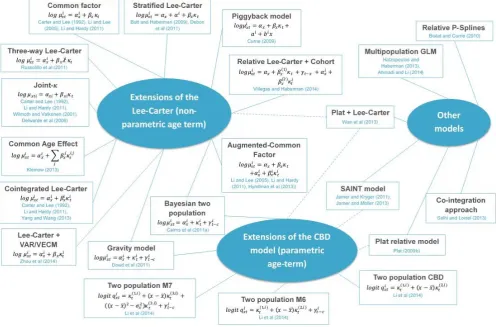
This section provides a general introduction to the available models to represent the mortality dynamics in the reference and the book populations. Figure 5.1 contains a schematic representation of the multi-population models currently available in the published literature, broadly grouped according to three main categories which we introduce in the next section.23

Figure 5.1: Universe of multi-population models

5.1 Literature review

Many models have been proposed in the literature to represent the mortality evolution of two or more related populations. All such contributions extend known single population models by specifying the correlation and interaction between the involved populations.

Although most of the academic contributions to the modelling of multi-populations are fairly recent, the first ideas go back to the seminal paper by Carter & Lee (1992), which suggested possible ways of extending their single population model in order to forecast differentials in US mortality between men and women.

Many existing models focus on the mortality rates of two or more related populations such as:

 National populations of different countries

 Men and women within a given country/population

 Smokers and non-smokers within a given country/population.

23

A review and comparison of multi-population models can be found in Li and Hardy (2011), Villegas and Haberman (2014), Danesi et al. (2014), and Li et al. (2014).

Some relevant papers are as follows:

 Li and Lee (2005) first explicitly formulated the joint modelling of two related populations using an extension of the Lee-Carter model where specific and common period terms are included.

 Li and Hardy (2011) contains a comparison of some models in the context of assessing longevity basis risk.

 Cairns et al (2011b) and Jarner and Kryger (2011) recognize the relative importance of the reference population backing the index and the population whose longevity risk is to be hedged. Therefore, the model focuses on the reference population first and then on the spread between the reference and the book.

 Li et al. (2014) compare several two population extensions of the CBD – M5, M6 and M7 type models.

Many of the models shown in Figure 5.1, including both the extensions of the Lee-Carter approach (based on a non-parametric age term) and of the CBD approach (based on a parametric age term), can be fitted into a common framework – see the next section. There are, however, other contributions in the literature which attack modelling multi-population mortality from a different point of view. For instance, Biatat and Currie (2010) extend to two populations the P-spline methodology that has been successfully applied in the single population case, while Hatzopoulos and Haberman (2013) use a multivariate GLM.

5.2 Modelling the reference and the book population: A general formulation

We have identified a general framework under which most models that have been introduced in the literature can be accommodated. However, in order to facilitate this comparison between models, the way such models are proposed here may slightly differ from their original formulation.

As in Jarner and Kryger (2011) we choose a “relative approach” where the reference population is modelled first, and then the book mortality dynamics are specified so as to incorporate features from the reference population. This relative approach has some interesting features:

 It allows data mismatch between the reference and the book.

 It is well suited to the usual situation of the reference population being considerably larger than the book population.

 Reference population models are readily available and extensively studied, so this part of the model may be well established; allowing the focus to be on making an informed decision for the book part of the model, whilst retaining a good fit to the reference population.

 It provides consistency of approach when modelling several books using the same reference population.

Recall that 𝐷𝑥𝑡𝑅 and 𝐷𝑥𝑡𝐵 are the number of deaths aged 𝑥 last birthday in the calendar year 𝑡 in the reference

5.2.1 Reference population

A general model for the reference population can be written as24

𝐷𝑥𝑡𝑅 ∼ 𝐵𝑖𝑛(𝐸𝑥𝑡𝑅, 𝑞𝑥𝑡𝑅) (1)

𝑙𝑜𝑔𝑖𝑡(𝑞𝑥𝑡𝑅) = log ( 𝑞𝑥𝑡 𝑅

1 − 𝑞𝑥𝑡𝑅) = 𝛼𝑥

𝑅_{+ ∑ 𝛽}

𝑥(𝑗,𝑅)𝜅𝑡(𝑗,𝑅) 𝑁

𝑗=1

+ 𝛾𝑐𝑅 (2)

Here:

 The term 𝛼𝑥𝑅 determines the reference mortality level for age group 𝑥.

 𝑁 is some integer, allowing the user flexibility on the number of components which contribute to the mortality trend for the reference population with:

- Each time index 𝜅_𝑡(𝑗,𝑅) contributing to the reference mortality trend.

- Each coefficient 𝛽𝑥(𝑗,𝑅) dictates how mortality in the corresponding age group 𝑥 reacts to a change

in the corresponding time index 𝜅_𝑡(𝑗,𝑅) i.e. it modulates the sensitivity of the reference population at different ages to the general trend.

 The term 𝛾𝑐𝑅 is the cohort effect in the reference population (for birth cohort 𝑐 = 𝑡 − 𝑥).25

5.2.2 Book population

Given the reference population model, the book population is then specified through

𝐷𝑥𝑡𝐵 ∼ 𝐵𝑖𝑛(𝐸𝑥𝑡𝐵, 𝑞𝑥𝑡𝐵) (3)

𝑙𝑜𝑔𝑖𝑡(𝑞𝑥𝑡𝐵) − 𝑙𝑜𝑔𝑖𝑡(𝑞𝑥𝑡𝑅) = 𝛼𝑥𝐵+ ∑ 𝛽𝑥(𝑗,𝐵)𝜅𝑡(𝑗,𝐵) 𝑀

𝑗=1

+ 𝛾𝑐𝐵 (4)

Note that we are modelling the difference in the (logit of) mortality in the book and the reference populations. Therefore:

 The term 𝛼𝑥𝐵 determines the mortality leveldifferences of the book population compared to the reference

population for age group 𝑥. Hence the mortality level in the book is𝛼𝑥𝑅+ 𝛼𝑥𝐵.

 𝑀 is some integer (generally less than or equal to 𝑁), allowing the user flexibility on the number of components which contribute to the trend in differences in mortality between the book population and reference population with:

- Each time index 𝜅_𝑡(𝑗,𝐵) contributes in shaping the difference in mortality trends.

- Each coefficient 𝛽𝑥(𝑗,𝐵) dictates how mortality differences for age group 𝑥 react to a change in the

corresponding time index 𝜅_𝑡(𝑗,𝐵).

 The term 𝛾𝑐𝐵 accounts for the differences in cohort effect in the two populations (again for birth cohort

𝑐 = 𝑡 − 𝑥). Hence the cohort effect in the book is 𝛾𝑥𝑅+ 𝛾𝑥𝐵

Depending on how the model is specified, identification constraints may have to be added to (1)-(4) in order to ensure that there is a single set of parameters which will yield a given set of mortality rates.

24 _{Here, we have chosen to work with one-year death probabilities 𝒒}

𝒙𝒕. Therefore, it is most natural to use the logit function and model

deaths using a binomial distribution. However, if interested in central death rates, mx, or the force of mortality, μx, then the general modelling

framework can be easily reformulated using a log link function and a Poisson Distribution.

25_{Note that equation (2) does not allow for an age-modulating factor in the cohort term. Models including such a factor have been}