A KNOWLEDGE-BASED APPROACH TO MAPPING ROADS
FROM AERIAL IMAGERY USING A GIS DATABASE
by
Ali Forghani, B.Eng (UM, Iran), M.Eng (UNSW, Australia).
A thesis submitted in partial fulfilment of the requirements for the degree of
Doctor of Philosophy
in
Surveying and Spatial Information Science Faculty of Engineering & Surveying
The University of Tasmania
Si
...1■4117.
Surveying & Spatial Information Science Faculty of Engineering & Surveying
University of Tasmania GPO Box 252-76 Hobart Tasmania 7001
Australia Fax: +61-3-62240282 Telephone: +61-3-62262134
DECLARATION
Except as stated herein, this thesis does not contain any material which has been accepted for the award of any other degree or diploma in any university nor, to the best of my knowledge and belief, does it contain any copy or paraphrase of material previously published or written by another person, except where due reference is made in the text of this thesis.
I Ali Forghani, hereby given consent that my thesis A Knowledge-Based Approach to Mapping Roads from Aerial Imagery Using a GIS Database to be made available for loan at the discretion of the Head of Department, and the University of Tasmania shall be authorised to allow a copy of all or part of the thesis for the purpose of study or research.
Date: 1/6/98 Ali Forg
ABSTRACT
Conventional image classification approaches may be inadequate for extraction of complex and spectrally heterogeneous land use classes from remotely sensed imagery. The integration of spatial data with remotely sensed data has the potential to improve significantly the reliability of feature classification. Thus it is informative to use contextual and textural information in the classification process.
This thesis describes a methodology developed to integrate GIS and aerial imagery in a manner that allows it to be used in a knowledge-based analysis system. Using a trial site and aerial photography, the methodology was implemented and tests indicate the technique works well in mapping of roads when roads pass through a rural area where the contrast is high, but fails in urban areas where the roads are confused with man-made structures.
Also, a supervised multispectral image classification of the trial site using colour aerial photography was carried out to compare the performance of a supervised multispectral image analysis with the decision tree analysis to map out roads over the trial site. A classification accuracy assessment shows that the overall classification accuracy was marginally lower than the decision tree analysis.
The GIS data used in the knowledge-base included a DTM and land use covers. For this research, part of the data was already available in digital format. In practice, it may be that a DTM and land use classification would need to be created from aerial photography or satellite imagery. It is in this context that the methodology developed here is most likely to improve significantly attribute-based classification.
The multi-layer database was interfaced with decision tree software for creation of a classification tree. The independent data set comprised six variables, representing the contextual, textural, and geometrical characteristics of the knowledge-based data. In the process of decision tree analysis, the input data was recursively partitioned into mutually clustered, exhaustive subsets which define the best response variable. The resulting classification tree was used to generate generic rules for implementation of an expert system.
The developed expert system was used to map out the spatial distribution of the grid data to show areas with roads (presence) and their background (absence). The output of this model is encouraging when applied over homogeneous rural scenes, but there are difficulties over heterogeneous urban areas. The results show that a framework of roads in a rural site mapped by this knowledge-based technique closely concurred with visual interpretation.
This research devised a general approach to solving problems of road identification. This approach can serve as a model for practitioners who are trying to do practical work in this field. By generating a hybrid system which locates many different databases and integrates many different sources of knowledge in attempting to identify a specific (man-made) geographic feature, and by utilising current artificial intelligence (AI) techniques to perform the classification, this research provides an early example of the techniques which will be in more general use in the areas of GIS and remote sensing in the future.
ACKNOWLEDGMENTS
This thesis is the result of the efforts, guidance, and patience of many people over the past three years. Although it would be impossible to acknowledge all who have supported this research, I would like to express my special gratitude to the following individuals:
My supervisors: Dr Anthony Sprent who provided constant support, constructive and valuable advice throughout this research, and Dr Jon Osborn for his close guidance, and encouragement throughout the long period of experimentation and analysis in the course of the research.
Associate Professor Richard Coleman, Dr Peter Zwart, and Dr Michael Roach contributed to the early stages of this research.
I should also express my appreciation to all staff and postgraduate students in the Department, especially Mr Robert Anders, Mr John Cate11, Mrs Margaret Stafford, Mr Antonius Wijanarto, Mr Ngoc Lau Nguyen, and Mr Matthew King who contributed in their own way to my student life in the Department.
I would also like to thank Mr Phil Collier at the Department of Computer Science & Electrical Engineering, University of Tasmania; Mr Ross Lincolne at the Space Image Unit of the Central Science Laboratory, University of Tasmania; and Mr Lee Belbin at Antarctic Data Centre Australian Antarctic Division, Tasmania, who provided support and advice.
The data provided by the Land Information Bureau of Tasmania for this research is gratefully appreciated.
In addition, the financial support of the Ministry of Culture & Higher Education of the I. R. of Iran is gratefully acknowledged.
TABLE OF CONTENTS
DECLARATION ii
ABSTRACT iii
ACKNOWLEDGMENTS iv
TABLE OF CONTENTS viii
LIST OF FIGURES xiii
LIST OF TABLES xvi
ACRONYMS xvii
CHAPTER 1
INTRODUCTION 1
1.1 General 1
1.2 Prior Work 5
1.3 Hypothesis and Proposed Approach 6
1.3.1 Stages of Research 8
1.4 Contribution of the Research 8
1.5 Organisational Outline of the Dissertation 9
CtiAnER 2 11
BACKGROUND: CLASSIFICATION AND FEATURE DETECTION 11
2.1 Image Analysis 11
2.1.1 Texture 15
2.1.2 Context 15
2.2 Machine Learning in Remote Sensing and GIS 16
2.3 Approaches in Linear Feature Detection 19
2.4 Expert Systems in Remote Sensing and GIS 22
2.5 Summary and Remarks 25
CHAFFER 3 26
DIGITAL IMAGE AND GIS DATA PROCESSING 26
3.1 Image Rectification and Registration 26
3.1.1 Geometric transformations 27
3.1.2 Orthophotography 31
3.2 Image Enhancement 35
3.2.1 Edge Detection 35
3.2.2 Thresholding 39
3.2.3 Mathematical Morphology 40
3.4 Integration of GIS and Remote Sensing 42
3.4.1 Data Acquisition for GIS 42
3.4.2 Data Structure for GIS 43
3.4.3 Data Conversion 46
3.4.4 Error Sources from Integration of RS and GIS Data 51
35 Summary 53
CHAPTER 4 54
BACKGROUND: EXPERT SYSTEMS CONSTRUCTION AND KNOWLEDGE-BASED
INDUCTION 54
4.1 Artificial Intelligence and Expert Systems Implementation 54
4.1.1 Definition and Background 54
4.1.2 Components of an Expert System 56
4.1.2.1 Knowledge Acquisition 56
4.1.2.2 Knowledge Representation 58
4.1.2.3 Inference Engine 59
4.2 Extracting and Representing Knowledge with Decision Trees 61
4.2.1 Background 61
4.2.2 Inductive Learning 62
4.2.3 Decision Trees 62
4.2.3.1 Induction of Decision Trees Algorithms 64
4.2.3.2 Decision Tree-Pruning and Accuracy of the Classification Tree 68
4.3 Summary 71
CHAPTER 5 73
STUDY AREA AND DATA SETS 73
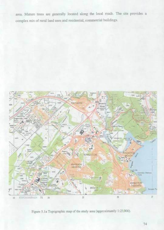
5.1 Study Area 73
5.2 Available Data 88
5.2.3 Base Maps 92
5.3 Computer Facilities 93
CHAPTER 6 97
IMAGE REGISTRATION AND LINEAR FEATURE DETECTION 97
6.1 Geocoding of Images 97
6.1.1 Polynomial Transformations 98
Technique Adopted 98
Experimental Results 100
6.1.2 Orthophotograhpy 101
Technique Adopted 103
Examining the Corrections 111
6.1.3 Affine Transformation and Rubber Sheeting 111
6.1.4 Discussion 113
6.2 Remarks for Image Registration 114
6.3 Linear Feature Detection and Analysis 115
6.3.1 Pre-Processing of Images 117
6.3.2 Image Segmentation 119
6.3.3 Analysis 122
6.3.4 Discussion 136
6.4 Remarks for Image Segmentation 141
CHAPTER 7 142
SPATIAL DATA PROCESSING: CONSTRUCTION OF A DATABASE FOR A KNOWLEDGE
BASED ENVIRONMENT 142
7.1 Spatial Data Construction 142
7.1.1 Data Entry 144
7.1.2 Database Development 144
7.1.2.1 Editing Road and Stream Coverages 145
7.1.2.2 Land Use Delineation 147
7.1.2.3 Rasterization and Resampling 149
7.1.2.4 Creation of Surface Data 149
7.1.2.5 Processing and Manipulating Raster Grid Data 150
7.1.2.6 Conversion of Raster Grid Data to ASCII Files 150
7.2 Summary 152
CHAPTER 8 153
EXPERT SYSTEMS DEVELOPMENT: DECISION TREES 153
8.1 Introduction 153
8.2 Developing a Knowledge-Based System 154
8.2.1 Basic methodology 154
Rule Induction 161
Inferencing 161
8.2.2 Input Data for Decision Tree Analysis 162 8.2.3 Decision Tree Environment and Interfacing a GIS Database 163 8.2.4 Generation of Decision Tree: Tree Growing and Analysing 163 8.2.5 Expert System Construction: Storage of Output of the Induction Rules 169
8.2.6 Analysis of Results 173
8.3 Discussion 180
8.4 Summary 183
CHAPTER 9 184
MULT1SPECTRAL IMAGE CLASSIFICATION 184
9.1 Introduction 184
9.2 Supervised Classification Method 185
9.2.1 Background 185
9.2.2 Image Classification 185
9.3 Discussion 187
9.4 Concluding Remarks 189
CHAPTER 10 190
SUMMARY 190
10.1 Background 190
10.2 Methodology 192
10.3 Results 196
10.4 Concluding Remarks 198
APPENDIX 223
APPENDIX A: DATA SETS INFORMATION 224
APPENDIX B: MATLAB CODE FOR PLOTTING THE COMPONENTS OF RELIEF DISPLACEMENT. 225 APPENDIX C: MATLAB CODE FOR BUILDING DATA FOR A KNOWLEDGE-BASED SYSTEM, USING EDGE ENHANCEMENT OPERATORS, EDGE DETECTION FILTERS AND MORPHOLOGICAL OPERATIONS
METHODS. 228
APPENDIX D: FORTRAN 77 CODE FOR GENERATING A TABULAR ASCII FILE FROM THE ARC/INFO
GRID ASCII RE,Es. 237
APPENDIX E: MATLAB CODE FOR DEVELOPMENT OF A DECISION TREE PROCESSING EXPERT SYSTEM (DTPES) TO MAP OUT THE SPATIAL DISTRIBUTION OF ROADS AND THEIR BACKGROUND FROM THE
GIS DATABASE 238
APPENDIX F: CROSS-TABULATION OF THE CLASSIFICATION TREE 250
LIST OF FIGURES
Figure 2.1 Image interpretation techniques classified according to segmentation level 14 Figure 3.1 Illustrates a rubber sheeting by using links and adjusting position 34 Figure 5.1a Topographic map of the study area (approximately 1:25,000) 74 Figure 5.1b Location of the study area in Hobart (Scale approximately 1:500,000) 75
Figure 5.2 Aerial photographs of the study area 77
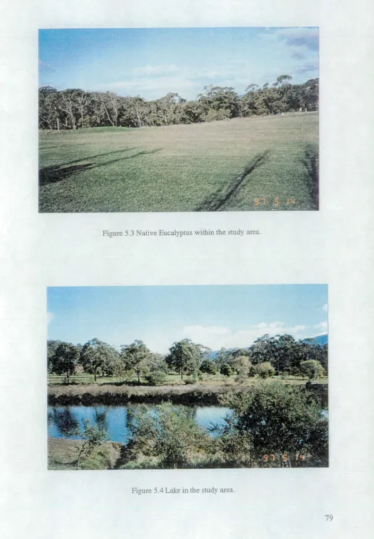
Figure 5.3 Native Eucalyptus within the study area 79
Figure 5.4 Lake in the study area 79
Figure 5.5 Land used for pasture in the study area 80
Figure 5.6 Golf course in the study area 80
Figure 5.7 Beach and ocean nearby the study area 81
Figure 5.8 Urban land use enclosed by rural land use 82
Figure 5.9 Semi-rural and urban development 82
Figure 5.10 Urban development for residential housing 83
Figure 5.11 Development of (a) industrial and (b) commercial areas in the study
area 84
Figure 5.12 Major access road in a rural area 85
Figure 5.13 Major access road in a semi-rural area 85
Figure 5.14 Major road in an urban area 86
Figure 5.15 Local road in an urban area 86
Figure 5.16 Asphalt road in a rural area with shadow from overhanging trees 87
Figure 6.1 Components of relief displacement 99
Figure 6.2 The vectors representing relief displacement for 1982 image plotted 99 Figure 6.3 Illustration of differences between the actual terrain and the maximum error in
Z coordinates (DEM) 102
Figure 6.4 Illustrates the DEM of the area as a grey scale image which was produced by
applying ARC/INFO TOPOGRBD tool 103
Figure 6.8 The geometrically corrected image using the affine transformations and a
rubber sheeting 112
Figure 6.9 Schematic of interactive linear feature interpretation of test area. 116
Figure 6.10 Test images; sub-sections of the 1982 image 117
Figure 6.11 Application of a median filtering 118
Figures 6.12 Represents application of Sobel filter with different threshold over a rural
site (a, b, c) and an urban site (d, e, f) 123
Figure 6.13 Mathematical morphology operations applied to the Sobel filtered data over a
rural site (a, b, c) and an urban site (d, e, f) 124
Figures 6.14 The result of Canny filtering for different threshold values with a filter of 7 by 7 over a rural site (a, b, c) and an urban site (d, e, 126 Figure 6.15 Morphological operation on detected edges from Canny filtering over a rural
site (a, b, c) and an urban site (d, e f) 127
Figure 6.16 The result of the Deriche filtering approach for different threshold values and
a =
0.5,a =1,a =
2, over a rural site (a, b, c) 130 Figure 6.17 The result of the Deriche filtering approach for different threshold valuesand a = 0•5,
a =1,a =
2, over an urban site (a, b, c) 131 Figure 6.18 Morphological operations over the produced Deriche filter edges over a ruralsite (a, b, c) and an urban site (d, e, f) 132
Figure 6.19 The result of Canny filtering for different threshold values with a filter of 7
by 7 134
Figure 6.20 Morphological operation on detected edges from Canny filtering 134 Figure 6.21 The result of the Deriche filtering approach for a threshold value of
40% and,
a
=2 135Figure 6.22 Morphological operations over the produced Deriche filter edges 135
Figure 7.1 Schematic of the data preparation 143
Figure 7.2 The study area 144
Figure 7.3 Road networks in a line form overlaid on the georeferenced image for a subset
of the study area 146
Figure 7.4 Road networks in a buffer form overlaid on the georeferenced image for a
Figure 7.5 Map of land use/cover of the area generated by manual interpretation of the
1982 air photo 148
Figure 7.6 A perceptive view of the synthetic surface of the area 149 Figure 8.1 Flow diagram of the expert system construction in this study 155 Figure 8.2 Part of a 65-rule model shows as a simple decision tree 165
Figure 8.3 Illustrates the end node for rule_17 170
Figure 8.3; (a) Displays the results from the clustering classifications for
Case 1 174
Figure 8.3; (b) Represents the road reference map of Case 1 in a grid, and (c) shows
the aerial image of Case 1 174
Figure 8.4; (a) Displays the results from the clustering classifications for
Case 2 176
Figure 8.4; (b) Represents the road reference map of Case 2 in a grid, and (c) shows
the aerial image of Case 2 176
Figure 8.5; (a) Displays the results from the clustering classifications for
Case 3 177
Figure 8.5; (b) Represents the road reference map of Case 3 in a
grid 178
Figure 8.5; (c) Shows the aerial image of Case 3 178
Figure 9.1 A subset of the colour aerial photograph of the study area 184 Figure 9.2 Represents the classified image with 9 classes. 186 Figure 9.3 Final supervised classification after merging of similar classes 187 Figure 1 (Appendix G) Shows a generated classification decision tree using clustering
LIST OF TABLES
Table 5.1 Computer facilities information 95
Table 6.1 A summary of results of rectification and registration of the aerial images using
polynomial transformations 100
Table 6.2 Representations of the DEMs and the maximum error in X and Y coordinates
due to DEM discrepancies in mm at photo scale 102
Table 6.3 Results of registering fiducial marks on the photo coverage 106
Table 6.4 Resection results 110
Table 6.5 Accuracy evaluation based on coincidence computations between the existing road map and the classified edge detection map for the rural site 137 Table 6.6 Accuracy evaluation based on coincidence computations between the existing
road map and the classified edge detection map for the urban site 138
Table 6.7 A summary of the results of edge detection 139
Table 6.8 Accuracy evaluation based on coincidence computations between the existing road map and the classified edge detection map for 1982 imagery 139
Table 7.1 Buffer distances and road class 147
Table 7.2 Land use/cover classification scheme for visual classification of B/W
photography 148
Table 7.3 Subset of a sample database for input into KS 151
Table 8.1 The seven variables or attributes (layers) existing in the database 160 Table 8.2 Sample of GIS data used for Decision Tree Analysis 163
Table 8.3 Classification summary statistics 179
Table 9.1 Selected signatures from the aerial image 186
Table 9.2 Image classification accuracy 188
Table 1 (Appendix A) Data sets information 224
Table 1 (Appendix B) Components of relief displacement for
ACRONYMS
Al Artificial Intelligence
AID Automatic Interaction Detector
AMG Australian Map Grid
B/W Black and White
BAY Binary
CART Classification And Regression Trees
CGIS Canada Geographic Information System
CIR Colour Infrared
DEM Digital Elevation Model
DEMs Digital Elevation Models
DGN Integraph Design Files
DN Digital Number
DPI Dot Per Inche
DTM Digital Terrain Modelling
DTPES Decision Tree Processing Expert Systems
ES Expert Systems
ERI Environmental Systems Research Institute
GC Ground Control Point
GCPs Ground Control Points
GIS Geographic Information Systems
GPS Global Positioning Systems
HMSDS Hybrid Model of Spatial Data Structure
ID3 Interactive Dichotomizer
lF0V Instantaneous-Field-Of-View
ILFDP Interactive Linear Feature Detection Program
KS ICnowledgeSEEICER
KB Knowledge-Based
ICBS Knowledge-Based Systems
LBS Learning Base System
LFC Large Format Camera
m Metre
MLC Maximum Likelihood Classifier
mm Millimeter
MO Morphological Operations
MSS Landsat Multispectral Scanner
NDVI Normalized Difference Vegetation Index
PAN Panchromatic
PCA Principle Component Analysis
PPA Principal Point of Autocollimation
RS Remote Sensing
RMS Root Mean Square
T Threshold
TDIDT Top-Down Induction of Decision Trees
TIN Triangular Irregular Network
TM Landsat Thematic Mapper
XS Multispectral
a Filter Size
2D Two Dimensional
Chapter 1
INTRODUCTION
1.1 General
Historically, land use/cover mapping has been undertaken using aerial
photography. Urban areas are a heterogeneous and complex environment which occupy
less than one percent of exposed land on the earth's surface. These areas represent both
natural and artificial human activities and contain both natural and man-made elements.
Consequently, urban land use patterns consist of objects with regular and irregular
shapes. Use of remote sensing (RS), in the form of aerial photography, in an historical
sequence in urban studies, dates back to 1858 when Tournachon (later named "Nadar")
used a camera set on a balloon to study parts of the city of Paris. Since World War II
increased consideration has been paid to the potential role of aircraft and satellite
remotely sensed data in the study of man-made and natural scenes. These studies have
produced classification accuracies ranging from 50-98% (eg Coleman, 1992).
Land cover mapping using airphoto interpretation has proven to be rapid, efficient,
and economical. There has been considerable effort given to its application in the
acquisition of data for resource management and civil engineering applications
throughout the world. Despite proven advantages of employing aerial imagery in urban
investigation, there are disadvantages in using this imagery. For example, manual
interpretation of aerial photography for a large area may be tedious and time-consuming.
In addition, the risk of different interpretations by various interpreters is a concern, as
well as the infrequency of data acquisition.
Aerial photography has been used for a wide variety of urban and rural studies, and
it provides the most effective method for the study of urban expansion and urban growth
analysis. The application areas include analysis of urban housing problems (Hathout,
1988), spatial location of waste disposal sites (Mack et al 1995), town planning (Mirsa,
1986), population estimation using 1:12,000 b/w photography (Lo, 1992), detection of
analysis of urban spatial structure (Hsu and Wu, 1990). Using colour infrared (ClR) imagery (Gong and Chen, 1988) the overall discrimination accuracy for urban expansion is 94.6%.
Mapping of land use and rural to urban conversions are topics of interest to both GIS and remote sensing communities. Specifically, mapping of road networks is a major research area in image and spatial data processing in order to update digital road network files. The problem of keeping road network files up to date is most acute in the urban fringe of major urban areas where development processes are most concentrated.
Medium level image segmentation operators such as edge detectors have been applied widely to extract linear features from remote sensed data (eg Boggess, 1994). The performance of the medium level operators is satisfactory (Forghani, 1997; Forghani et al 1997). The interface of contextual information by means of incorporation of GIS data and human knowledge-base leads to better quantitative accuracy. The interface of GIS and remote sensing data for classification and feature extraction by machine learning' methods (ie decision trees and artificial neural networks) and expert systems (ES) is a major area of research in a knowledge-based (KB) integration of image and spatial data. The results obtained from any single analysis can be subjected to error and are imprecise.
Multispectral image classification approaches have been shown to be inadequate for extraction of complex and spectrally heterogeneous land use classes from high resolution remotely sensed imagery (Barnsley and Barr, 1996). However, in spite of the large body of previous research in this area and a number of comparative studies, the choice of algorithms suitable for complex imagery is not clear. The way forward appears to be to use both contextual and textural information in the classification process (eg Johnsson, 1994).
Integration of image understanding techniques within a GIS database have been modelled to govern feature extraction problems, eg Gahegan and Flack (1996). Integrating different analyses of feature extraction improves the results, particularly in complex scenes like urban areas. Little interest has been shown concerning feature extraction (ie roads) using non-parametric methods, eg decision trees. Extension of ES has been successfully presented in combining image processing techniques with a GIS data base for extraction of roads (eg Van Cleynenbregel et al 1990).
Decision trees2 have been developed both by the statistical community (Hunt, 1962) and artificial intelligence community (Quinlan, 1983, and 1986). The main limitation of these learning systems is that extrapolation is unreliable, but they can provide reasonable interpolation within the learning example (Lees, 1994). In this research the KnowledgeSEEKER (KS) software was used because it is a simple and widely used symbolic algorithm for learning examples. It has been comprehensively examined on a large number of data sets (De Ville, 1990) and is the basis of several commercial rule induction systems. Moreover, KS has been improved with methods for handling numerically-valued features, noisy and incomplete data, and missing information (ANGOSS, 1994).
A technique has been developed to integrate the information obtained from the different sources. To integrate the aerial photographs into a GIS the images, were geometrically corrected using an affine transformation and rubber sheeting. The rectified images were used for identifying linear features by edge detection and mathematical morphology. In the development of the methodology of this research, an Interactive Linear Feature Detection Program (ILFDP) was developed for semi-automatic linear feature detection using different edge detectors, followed by morphological operations (Forghani et al 1997; Forghani and Osborn, 1998b). The extracted edges were used as a GIS layer in a later step of the methodology A knowledge-based data set which locates spatial and spectral attributes was created using ARC/INFO GIS software.
Grid raster-based processing was undertaken to construct the multi-source database. After the gridding process, seven principal map features (layers) were created, namely land use/cover, DEM, grey image, roads, field boundaries, streams, and edge detection data. To input the data into KS it was necessary to convert multiple ASCII files using sources such as land use/cover hydrographic maps, aerial imagery, and digital elevation model (DTM) as well as the medium level image segmentation product (ie extracted edges) held in a GIS to be used in a knowledge-based environment to predict distribution of roads using decision trees.
1.2 Prior Work
In the last decade there has been a rapid increase in the development and application of the machine learning approach. Civil engineers, mapping specialists, computer scientists, natural resource managers and environmental science experts are involved, with increased use of machine learning for data analysis, modelling and mapping (Moore et al 1991; Aspinall, 1991 and 1992; Skidmore et al 1996a) employing GIS and remote sensing imagery.
The application of decision trees in the use of remotely sensed images and GIS data for environmental applications has been widely discussed. Key references are, Walker and Moore (1988) for mapping of wildlife distributions, Reddy and Bonham-Carter (1991) for mapping of spatial distribution of mineral occurrence, Lees and Ritman (1991), Moore et al (1991) for vegetation mapping, and recently Skidmore et al (1996b) for classification of kangaroo habitat distribution.
1.3 Hypothesis and Proposed Approach
This thesis describes a methodology developed to integrate GIS data and aerial imagery in a manner that allows it to be used in a knowledge-based analysis system for detecting and mapping linear topographic objects, particularly road networks. The research uses photometry (ie spectral) or textura1 3, spatial and contextual information (contextual-based4 attributes) within a knowledge-based model using decision trees.
Geometric, spectral, and spatial characteristics are applied to distinguish roads from other linear features (eg rivers, field boundaries). The above information is located in a multi-source spatial dataset (layers) which includes land use/cover, DEM, grey level image, roads, field and vegetation boundaries, streams, and edge detection data. Incorporation of this dataset into a decision tree analysis system was attempted.
This research devised a general approach to solving problems of road identification. This approach can serve as a model for practitioners who are attempting to do practical work in this field. By creating a hybrid system which includes many different databases and combines many different sources of knowledge in trying to identify a specific (man-made) geographic feature, and by utilising current artificial intelligence (Al) techniques to perform the classification, this research provides an early example of the techniques which will be in more general use in the areas of GIS and remote sensing in the future.
The methodology was implemented for a trial site that contained a mix of urban and rural land uses. The study site is located on the southern fringe of Hobart, Tasmania, Australia. The trial site has a number of settlement types including suburban fringes, farms, residential, and commercial areas.
3 Textural attributes in this research include edge detection data and intensity.
Experiments show the technique works well when mapping roads within rural areas where the contrast is high, but fails in urban areas where the roads are confused with man-made structures.
In addition, a supervised multispectral image classification of the trial site using colour aerial photography was undertaken to compare the performance of a supervised multispectral image analysis with the decision tree analysis to map out roads over the trial site. A classification accuracy assessment shows that the overall classification accuracy was marginally lower than the decision tree analysis.
During the development of the methodology, several issues have been considered. These are:
Defining the dataset.
What are the most appropriate spatial data layers to use in the dataset? Building the spatial dataset:
How can a dataset that recognises knowledge-based attributes (data layers) such as intensity, elevation etc. be built for a decision tree environment in order to distinguish roads from other linear features? Which geometric correction method may produce better accuracy? Which type of spatial data structure can be employed in order to
manipulate and organise the vector and raster GIS data to build a dataset for KS software?
What cell size should be chosen to meet the requirements of the knowledge-based data?
Interfacing GIS data with the decision tree program:
What is the best way to transfer GIS datasets into the decision tree software?
Converting results of the classification tree into a classified image, since the decision tree software gives the results of classification tree both in generic rules and in graphic form:
1.3.1 Stages of Research
The following steps have been undertaken in this research:
Definition of the goal which deals with the development of the methodology and its implementation for a trial site for mapping roads.
Selection of suitable hardware and software to do the processing. Selection of an appropriate study area.
Selection and acquisition of the datasets and georeferencing of the aerial imagery. Definition of the dataset.
Spatial data processing and construction of a database for a knowledge-based analysis system.
Transferring of the data with a decision tree environment.
Decision tree analysis; generation of a classification tree and rules collection and encoding to develop an expert system.
Expert systems construction and testing of the expert system over trial sites. Multispectral image analysis.
1.4 Contribution of the Research
Updating maps of roads in any region of the world is required for a wide range of civil engineering and environmental planning purposes. This research describes a methodology developed to integrate spatial data and aerial imagery in a manner that allows it to be used in a knowledge-based analysis system.
This research contributes to the field of knowledge in this area as follows:
It provides a clear demonstration of the problems associated with georeferencing aerial imagery to suit an integrated spatial data model for delineation of linear features in rural and urban areas.
morphological operations (eg dilation) to aid geometric structuring of edge segments. This was implemented as a first step in building data for a knowledge-based environment.
It implements an integrated GIS (vector data) and RS (raster image) data model to construct a dataset for a decision tree environment, particularly one that recognises knowledge-based attributes such as spectral and spatial information in order to distinguish roads from other linear features.
It describes the interfacing of GIS data with a machine learning environment to construct a classification tree. This phase is important in deriving knowledge from classification trees. Development and construction of an expert system for mapping road networks using generated decision rules was attempted. Evaluation of the decision tree performance both over urban and rural sites was undertaken.
It provides a comparison of a standard supervised multispectral image classification techniques with the decision tree analysis to map out roads over a trial site.
1.5 Organisational Outline of the Dissertation
This thesis is organised into 10 chapters. In this first chapter, the research has been placed in a general context, the basic hypothesis and proposed approach have been demonstrated, and the original contribution of the research presented.
Chapter 2 introduces the major concepts which form the basis for this project, and includes a brief review of image segmentation and classification in the context of feature detection with special emphasis on road extraction using machine learning and expert systems.
Chapter 3 presents solutions for geometric correction errors of aerial imagery, image enhancement and classification methods including edge detection, thresholding, and morphological operations. It then provides an overview of integrated GIS and RS.
Chapter 5 describes the study area, the available data including GIS data and aerial imagery, and the hardware and software which was used.
Chapter 6 deals with digital image processing; pre-processing of the data sets such as georeferencing of the aerial photography, and processing of the data such as image segmentation via developing a computer program for primitives extraction.
Chapter 7 describes the process used to construct a database for knowledge-based software. The integration of GIS data and remote sensed imagery is considered. A grid raster-based processing was undertaken, and then the grid data were preprocessed by writing a computer program to generate a tabular ASCII file.
Chapter 8 demonstrates the decision tree analysis, and consequent rules collection from the generated classification tree to develop a decision tree processing expert system. In this chapter, two routines are implemented: (1) the first program translates the generated generic decision trees rules to MATLAB programming statements, and prints them in a file, and (2) the second program executes the rules against the datasets to map out the roads and their background, and finally computes the overall classification accuracy based on the reference data.
Chapter 9 describes a supervised multispectral image classification of the trial site using colour aerial photography. The aim was to compare the performance of a standard technique image classification technique (supervised multispectral image analysis) with a decision tree analysis to map out roads over the trial site.
Chapter 2
BACKGROUND: CLASSIFICATION AND FEATURE DETECTION
This chapter reviews image segmentation, using textural and contextual information, machine learning techniques and expert systems (ES) in geographic information systems (GIS) and remote sensing (RS) for feature extraction and classification. The main emphasis is on road detection incorporating decision trees.
2.1 Image Analysis
In the design of an image understanding system, a distinction must be made between different levels of image processing and their impacts. There are two major types of image analysis in the classification of remote sensed imagery (Moller-Jensen,
1990). (1) Synthesizing: its aim is to retrieve overall information about the main spatial trends in the data such as the extension of industrial areas (eg Forghani, 1994). (2) Analytical: the objective is to register information about the smallest elements in the data set such as housing units (eg Forster, 1993). Artificial intelligence methods of information extraction, knowledge representation, and symbolic reasoning can be applied to achieve this aim (Wang and Newkirk, 1988). The spatial resolution of input image plays an important role in the process of feature extraction. For example SPOT data may be suited to the analytical approach because it shows detailed information, whereas Landsat TM data is more appropriate for the synthesizing approach.
I) Low Level; requiring no intelligence on the part of image interpretation. Low level image segmentation methods can be grouped into two phases:
Image acquisition which requires two elements, namely a physical device and a digitizer to convert the electrical output of the physical device into digital form.
Pre-processing; this phase can be divided into radiometric processing eg histogram equalization, and geometric processing eg polynomial transformation. A number of transformed data sets such as principle component analysis (PCA), normalized difference vegetation index (NDVI) have been used in multispectral image analysis eg for change detection (ie Fung, 1992). Since this thesis will not consider multispectral image analysis in depth, these techniques are not discussed here. Detailed discussion of these techniques is provided in (eg Richards, 1986; ERDAS 1994b; Forghani,
1993). Geometric processing is discussed in Chapter 3.
II) Medium Level; the intermediate level deals with extraction and characterization of the constituent components of an image such as scene description. The medium level process is described as simple aggregation of the basic primitives such as edges and lines. Image primitives do not have any semantic information, but can be meaningful and sufficiently incorporated in high level of representation by using meaningful objects to allow image representation in terms of the aims of the analysis. A prime example of this algorithm is neighbourhood operators which examine the value of a small neighbourhood of pixels around a given pixel and generate a resultant value that is a function of all pixel values in the neighbourhood (Argialas and Harlow, 1990). The image primitives (Marr,
(based on a priori knowledge) from the operator or not (based on similarity assumption). These techniques have been widely discussed in remote sensing texts (eg Richards,
1993).
Low Level
Image Acquisition
Satellite sensors, scanners
Pre-Processing 1) Radiometric Processing
Image Enhancement - Histogram equalization, - Median filtering for noise removal - Multispectral (ie Landsat TM); PCA, NDVI 2) Geometric Processing (eg polynomial transformations)
}
Ii
Medium Level
Scene Description:
Edge Detection (eg Sobel, Marr-Hildreth, Canny) Thresholding
Line Detection (eg Hough Transform) Curve Detection
Point Detection Line/Arc/Curve/Edge Linking
Mathematical Morphology Boundary/Region Detection
Supervised Classification (based on a priori knowledge; supervised and heuristic learning: multispectral image, texture, context)
Unsupervised Classification (based on Similarity Assumption: Clustering, and unsupervised learning; image segmenting ie contouring, regioning, labelling of image elements ie pixels,
contours, regions) Region Growing
Split and Merge Relaxation Labelling Hybrid Models Texture Segmentation Shape Detection/Identification
4
, High LevelScene Analysis Using a Knowledge-Base Fuzzy Sets Theorem
Certainty Theorem
Machine Learning (Decision Trees, Neural Net, Genetic Algorithms) Frames and Rules
Production Rules
Artificial Intelligence/Expert Systems Object Orientation
[image:32.568.82.495.86.728.2]Hierarc hical/Relational Databases
2.1.1 Texture
Texture describes the smoothness of an object or a part of an image. Also it can be described as structure composed of large numbers of more or less ordered similar objects or patterns without these drawing particular consideration (Van Gool et al 1985). Texture can be used to delineate regions, boundaries in image segmentation, object identification, and to characterize the tonal or grey level variation in an image (Wang and He, 1990). There are many approaches and models for texture analysis in image processing. Algorithms for texture analysis have been developed by many authors including Haralick (1979); Harlow et al (1986); Franklin and Peddle (1990). These include statistical approaches such as autocorrelation (Haralick, 1979), optical transforms, digital transforms, textural edge operators, structural elements (eg Haralick and Shapiro, 1985; Franldine and Peddle, 1990), grey tone occurrence (eg Gong et al 1992), run lengths, and autoregressive models (Haralick, 1979). Reed and Du-Buf (1993) provide a comprehensive review of the literature in this field.
2.1.2 Context
The main objective of using context in linear feature extraction is to improve the accuracy of image classification results. Considerable efforts have been made by Wang and He (1990), Johnsson (1994) and Ko (1995) to develop and improve classification of image data using contextual information.
2.2 Machine Learning in Remote Sensing and GIS
Machine learning methods such as non-parametric methods have been used to integrate analysis of GIS and remote sensing data. They can be grouped into three distinct areas:
artificial neural networks, genetic algorithms, and decision trees.
This research will deal with decision trees. Neural networks are used to recreate biological information processing methods in software. The paradigm of artificial neural systems is based on the way the brain processes information. A simple model of a neural network consists of (i) input layer where values are applied to the inputs, changed, based on some mathematical rule and then accumulated at the nodes; (ii) output layer where the inputs are processed and classified. The sum can then be functioned mathematically again before it is applied to the output. Each dendrite in the brain acts as an input to the neuron; and a hidden layer. The nodes (neurons) are connected with weights that are adjustable during the learning process, and adjustment takes place to improve the performance of the neural network. The neurons and weighted links between these neurons simulate synaptic activities. One of the most common neural network models is the back-propagation that has been under experiment in land cover classification problems. The model neurons can be connected into networks in widely varied ways. Michie et al (1994) provide a detailed discussion of the theoretical viewpoints on this technique.
1995), signalized point recognition in aerial photographs (Kepuska and Mason, 1995). More importantly, Boggess (1993, 1994) and Ko (1995) applied artificial neural networks for identification of roads from Landsat TM imagery. Artificial neural networks have drawbacks in the slow learning process that is initially related to a back-propagation training scheme. However, solutions can be found by developing a dynamic learning neural network to perform classification (Chen et al 1995).
Decision trees use a contextually-based approach which incorporates decision rules and spatial relationships of attributes (if they are input to the process) to classify objects (Walker and Belbin, 1990). The authors conclude that incorporating more spatial relationships into a GIS is more effective using clustering methods. The decision tree facilitates grouping large numbers of observations and subsequently translates group membership into classification rules which provides effective analytical tools for the GIS user.
Decision tree analysis has been applied for mapping mineralisation based on a GIS multi-map overlay using cluster and exhaustive partitioning'. It was reported that the exhaustive method provided better results over the cluster model (Reddy and Bonham-Carter, 1991). Also, Moore et al (1991) have applied decision trees with a GIS data base for prediction of vegetation distribution. They confirmed the value of decision tree analysis and cartographic modelling for environmental mapping.
An inductive modelling technique has been applied for analysis of wildlife patterns in spatial data (Landsat TM data and DTM) and employs a Bayesian statistical approach to develop a GIS for habitat mapping (Aspinall, 1991). The research used a spatial modelling procedure operating within GIS and introduced a significant learning capacity. Aspinall (1992) concluded that this modelling technique offers significant potential in mapping and management of the environment. Also Stockwell (1993) developed a learning base system (LBS) classifier for the purpose of automatic mapping in a GIS such as automatic mapping of wildlife distribution, and diagnosis of diseases by acquisition of knowledge from an expert. The Bayesian algorithm proved to be a flexible method for conducting an extensive variety of knowledge-based tasks (Stockwell, 1993).
In addition, two techniques of machine learning including decision trees (ID3 and CART) and genetic algorittuns 2 were conducted for analysis of natural resource data in terms of investigation of lake acidification. The result_ of the survey showed that both the decision tree and genetic algorithm approach seemed to be appropriate methods for identification of lake acidification (Liepins et al 1990). Recently, Skidmore et al (1996) attempted to compare three methods for mapping wildlife, so-called BIOCLIM, CART (decision trees) and a non-parametric classification technique employing a GIS dataset.
1 Cluster method refers to two-way partitioning or pair-wise merging (binary tree) which clusters values of partitioning variables together and finds the maximum similarity within the groups and dissimilarity between the groups.
Exhaustive method refers to a multi-branch technique which identifies the codes that form the nodes and branches of the classification tree. These choices generate a split for each potential partitioning variable. Further details can be found in De Ville (1990).
Among these techniques, the decision tree provided the most accurate result, but was costly to implement.
Apart from the above discussed areas, fuzzy set theory to image classification and accuracy assessment of thematic maps (eg Gopal and Woodcock, 1994) have been applied. An algebraic approximation to the generating appropriate classification with fuzzy attributes has been provided in Gisolfi and Nunez (1993). The fuzzy set theory emerged in the 1960s to describe the imprecision that is characteristic of much human reasoning, particularly in domains such as pattern recognition and information abstraction. It has been successfully applied to pixel or subpixel classification (Wilkinson and Megier, 1990). In addition, applying the theory of evidence is reported by (Shafer, 1976) for classification purposes. The theory of evidence relies on a numerical integration function to add to the evidence and has been performed in some problems of mixed spatial data. However, due to its numerical basis, it has limitations for use in some situations which would not themselves simply to the incorporation of non-numerical map-like data in terms of being subjective and inconsistent in generating the prerequisite evidence (Sirinvinsan and Richards, 1993; Peddle, 1995). This problem can be overcome by applying a more subjective approach for deriving evidence from histogram bin transformations of supervised training data frequency distributions (Peddle, 1995).
23 Approaches in Linear Feature Detection
Linear features in remote sensing imagery include roads, rivers, bridges, vegetation alignments, field boundaries, shorelines, and geologically significant features such as faults and joints. Fundamentally, there are two techniques used to detect these linear features.
which is shifted over a region and compared to the corresponding grey levels (eg Domenikiotis, 1994). The Hough Transform is a line detection method used by various researchers (Wang and Liu, 1994; Aghajan and Kailath, 1994) to detect roads and lines. Line tracking algorithms track roads by using seeds from an image. Papers dealing with road tracking models include those by Fischler et al (1981); McKeown and Zlotnick (1990); Geman and Jedynak (1996). Although these models vary in their detail, all assume prior knowledge of the location of linear structures and are based on that domain knowledge, and generate more information on the road networks.
2) An edge detection approach may be fruitful if the user is concerned with representing the exact size of the road. If roads have significant width (ie 2 or more pixels width), it may well be more useful to employ an edge detector in order to derive edges of roads rather than the centre line (Domenikiotis et al 1995). Edge detection and filtering (eg Nevatia and Babu, 1980; Schanzer et al 1990), contextual filtering (eg Vanderbrug and Rosenfeld, 1978; Gurney and Townshend, 1983) and mathematical morphology (eg Destival, 1986) have been discussed and applied for feature extraction (eg Destival, 1986).
Employing knowledge sources such as photometry and perceptual grouping (eg Tavakoli and Bajcy, 1976; Van Cleynenbreugel et al 1990; Domenilciotis, 1994), global land cover classification (ie Ehlers et al 1990; Stadeimam and Lodwick, 1993), existing roadmaps, drainage networks maps and a digital terrain model (ie D'Agostino et al 1993; Skidmore et al 1996) can be expected to improve the reliability of road detection and classification routines. Two main types of knowledge sources have been used: photometry and perceptual grouping rules (eg. Pai et al 1986; Wang and Newkirk, 1988; McKeown and Zlotnick, 1990; Van Cleynenbreugel et al 1990).
To delineate a road, an image interpreter may apply structural, spectral, and contextual knowledge (Swain et al 1980). Structural knowledge of roads has been examined with incorporation of computer systems, and by a GIS-guided technique (Van Cleynenbreugel et al 1990). Researchers are using the following properties to aid road detection:
spectral characteristics, geometric shape, and spatial properties.
information as an intermediate image segmentation level. It would appear that this method has difficulties in accurate detection of roads over a mixture of man-made structures. A more comprehensive discussion of road detection applying neural networks for combining multi-source evidence is provided by Boggess (1993 and 1994) and Ko (1995). In addition, genetic algorithms have been applied to classify roads in satellite imagery, and the results have been compared with a neural network technique (Boggess,
1990).
Recently, Geman and Jedynak (1996) presented a new method for tracking roads from SPOT images. The approach was related to the recent work in active vision on where to look next and associated with the divide and conquer method of parlour games. The general methodology dealt with decision trees and the role of entropy in pattern recognition. In this approach intensity and geometry are considered in the process of road detection. Implicit in Geman and Jedynak's approach (1996) was the concept of the decision trees. The approach was shown to work well for tracking major highways, but it had difficulty tracking the smaller roads due to the fact that roads were confused with other man-made structures.
2.4 Expert Systems in Remote Sensing and GIS
A number of applications of Knowledge-Based Systems (KBS) are concerned with analysis and processing to develop rule-based techniques. Several systems have been designed in artificial intelligence (Al) and ES to provide support for integration of GIS and remotely sensed data (eg Pal et al 1986; Stadelmann and Lodwick, 1993; Skidmore et al 1996a). Application of ES techniques in the domain dealing with spatial data has been widespread. For example, Skidmore et al (1996) conducted an expert system approach for mapping forest soils by utilizing a DTM, vegetation map, and knowledge provided by a soil scientist. This technique provides an accuracy of 70% which competes with a map drawn by the soil scientist.
The use of knowledge-based methods in current applications of GIS seems a little more than ad-hoc application of strategies initiated in the area of Al (Smith and Yiang, 1991). There is a wide variety of contemporary literature that deals with knowledge-based approaches such as the theory of evidence, machine learning methods, fuzzy logic for GIS and RS applications. An idea of how the scope of GIS can be developed by employing techniques from an AT context that can resolve the constraints and problems in user interfaces mainly by data representation and its visualization in the process of integration of remotely sensed imagery and GIS data, has been illustrated in many articles (McKeown, 1987). Image processing techniques alone are inadequate if in a situation where specific information or prior knowledge about the scene in question is required.
been identified as a facilitative tool which enhances the power of GIS. These parameters are related to the following areas (Smith and Yiang, 1991):
ICBS, defined in terms of languages that support knowledge representation and deduction, will not add any new expressive or computation power to the current languages employed in GIS.
In connection to the acquisition, ICBS enhances the construction of applications in the context of automization of procedural knowledge capture.
ICBS techniques for storage of GIS databases have been employed.
KBS made an easy mechanism to use GIS in the process of access such as query optimization and the use of metadata. The query optimization is extremely significant for large-scale GIS modelling involving complex multi-component and nested spatial objects in which features may be implicitly represented in a multi-layer data model. KBS facilitate the building of natural language interfaces, and these languages provide an easy way to use GIS in the process of interfaces.
The topics of data acquisition, data structures, and problems of data conversion will be discussed in Chapters 3 and 7. The interface of GIS and RS in a ICBS model for methodology developed in this research will be elaborated in Chapter 8.
The rule-based expert systems approach is another attractive method of road extraction. Pal
2.5 Summary and Remarks
A number of image segmentation approaches have been discussed, starting with image analysis, segmentation methods, using textural and contextual information, extension of machine learning and ES into feature extraction, and knowledge-based approaches to road detection. Consequently a review of classification (segmentation) methods leads to identification of four basic operations:
Incorporating radiometric and geometric enhancement for image interpretation Applying contextual information
Incorporating textural information
Employing semi-automatic and automatic approaches using artificial intelligence and machine learning techniques, particularly artificial neural networks, decision trees, genetic algorithms, fuzzy logic, theory of evidence, and expert systems.
Chapter 3
DIGITAL IMAGE AND GIS DATA PROCESSING
This chapter provides a review on integration GIS datasets and RS imagery, giving emphasis to data conversion problems, particularly the problems associated with geometric distortions of digital aerial photographs. These later problems are discussed and standard methods for their geometrical correction are presented. The subject of image enhancement using edge detection and mathematical morphology is reviewed.
3.1 Image Rectification and Registration
Image registration is the process of spatially best aligning two views of a scene captured using similar or dissimilar sensors (Pratt, 1978; Kanal et al 1981; Ton, 1989). Georeferencing is the process of establishing a best fit between an image (row, column) coordinate system and a map (x,y) coordinate system (ERSI, 1992d). This involves warping the geometry of the image in order to establish the same relationship between the image and map coordinates.
Image rectification is the process of geometrically correcting systematic and random distortions in an image to fit ground control (Lillesand and Kiefer, 1987; Goshtasby, 1987 and 1988). Image rectification is a common problem arising in digital image processing and GIS applications whenever the image and the ancillary data of the same scene have to be compared pixel by pixel.
Distortions in aerial photographs are caused by changes in ground elevation, camera (sensor) position and orientation, lens distortion, earth curvature, film distortions, and atmospheric refraction (Wolf, 1988; Zhizhuo, 1990; Frost, 1995). These distortions need to be corrected before an image can be used for remote sensing and GIS applications. The aim is to provide a photo as free from errors as possible.
Image rectification and image registration are crucial when undertaking the following:
change detection (eg Milne, 1988; Forghani, 1993; ERDAS 1994a)
scene classification and analysis (eg Silfer, 1988; Della Ventura et al 1990)
image or feature enhancement (eg Ford et al 1983; Goshtasby, 1987; Ehlers et al 1990)
depth perception (Goshtasby, 1987)
GIS data entry (eg Johnson, 1989; ESRI, 1992d).
For topographic map production, reliable spatial data is produced from aerial photographs using stereo-photogrammetric techniques. For GIS applications there are three common types of geometric rectification applied to digital images:
Geometric (polynomial) transformations are applied when image
distortions are highly systematic and relief displacement is not significant. Digital orthophotography, which is applied when there is significant relief displacement. A Digital Elevation Model (DEM) is used to resample an image and produce an orthographic projection of the terrain.
Affine transformation and rubber sheeting which is based on point matching of the two sets of points by applying a rubber sheeting process.
3.1.1 Geometric transformations
(i)Ground Control Points Selection
Image features commonly used as GCP include points on roads, rivers, field boundaries, shorelines, and power lines sometimes, using a visual fit of curved tracings to sections of the physical features in the image and referenced map. The use of GCP's to register remote sensed images to a georeferenced map is described by, for example, Welch and Usery, (1984); Labovtiz and Marvin, (1986); Marvin et al (1987).
Manual selection of GCP which depends on the visibility of invariant physical features such as line intersections and points. Numerous researchers have addressed the problem of control point selection (eg Welch, 1985; Marvin et al 1987; Mather, 1995).
Semi-automatic and automatic methods such as point and line matching, relaxation labelling schemes (eg Goshtasby, 1988; Ton, 1989; Li et al 1993)
The number of GCP's used and their position in the image depends upon the type of terrain and a variety of other factors. It has been shown elsewhere that polynomials are an effective way of correcting different types of image geometric distortions in digital images (Van Wie and Stein, 1977; Usery and Welch, 1989). There is a relational formula for the number of required GCP and the order of transformation (Labovtiz and Marvin,
1986). A minimum practical number of GCP's is required to calculate a transformation (Welch, 1985). A useful formulation is shown below (ERDAS, 1994b):
GCP = (t1 +1)(t + 2) (3.1)
2
where t is the order of transformation.
Provided that sufficient accuracy is obtained, a low order transformation is preferable due to the fact that few GCP are required to register the image on to a map. The number of GCP required is dependent on terrain type, scale, and the required level of accuracy.
An image with low spatial variation, often a low order bivariate polynomial (m = 2 or 3) is a good approximation to the actual situation. Larger geometric variations need higher order polynomials to gain a given error tolerance. Generally, the coefficients associated with higher order in the polynomial are sensitive to the location of the GCP, which has to be uniformly distributed throughout the image. This problem can be avoided by employing orthogonal polynomials ie Legendre or Hermit polynomials. Coordinate transformations are an approximation of the true values.
Root Mean Square (RMS) errors can be used to evaluate the performance of least squares fitting routines. The root-mean-square error (RMS) is a measure of accuracy for each GCP in the image and can be written (Domenikiotis, 1994):
Once the transformation for a given GCP is performed, the suspect points from the total RMS error, the X and Y residual, and contribution table can be examined and errors detected and eliminated. The pair point distances 1 are then computed and the RMS difference values identified. The RMS errors reflect the reliability of GCP's, and are an index of the internal geometric fidelity of the image data.
Lincolne (1995) and Forster (1995) report if the GCP come from a 1:25,000 scale map, it can be expected that the GCP will be accurate to 0.5 mm (obtaining error values of about ±12.5 m on a 1:25,000 scale topographic map). Della Ventura et al (1990) gained an accuracy of 2.57 RMS error pixel and 2.68 RMS error pixel using 8 automatically detected GCP and 11 manually detected GCP's respectively.
(ii) Resampling
Resampling can be described as the process of adjusting the location of pixel centres for generating an image (grid) at a predetermined scale and with attribute values derived from the original data. Three common methods of polynomial transformation are cited in the literature, and these techniques have been applied in image (grid) data which are available in GIS (eg ARC/INFO) and remote image processing software (eg ERDAS IMAGINE):
Nearest-neighbour Bilinear-interpolation Cubic-convolution
In addition, interpolation techniques such as bilinear interpolation and weighted Brownian interpolation 2 have been extended to digital elevation models (DEM) (eg Ungar et al 1988; Polidori and Chorowicz, 1993).
Pair point distances are a comparison of map and scaled photo distance between all alternative combinations of point-pairs.
2 Brownian interpolation refers to a Random Midpoint Displacement algorithm, described by Polidori and Chorowicz
A nearest-neighbour assignment is computationally the fastest and easiest method to use of the three methods of interpolation. Primarily it is applied for categorical data such as land use classification, since it preserves the exact value of pixels in the original dataset values without averaging them, and therefore does not introduce new grey values. This is an important issue when discriminating between vegetation classes, locating an edge associated with lineament, or identifying different levels of turbidity or temperatures in a lake (Jensen, 1986). It suffers from some disadvantages as follows:
it introduces spatial shift errors such that local geometry can be inaccurate by up to
— of ground grid size (Lodwick and Pain, 1986), so that the maximum spatial error 2
will be one half the cellsize of the grid.
in resampling a larger to smaller grid size, there is usually a "stair stepped" effect around diagonal lines and curves.
also some data values may fall, while other values may be duplicated.
in addition, on linear thematic data (ie roads, streams) gaps or breaks in a network of the linear features may result.
A bilinear-interpolation determines the new value of a cell based on a weighted distance average of the four nearest input cell centres. This method tends to give more natural looking images, without the blockiness of nearest-neighbour or the over smoothing of the cubic convolution option, although there is a risk of information loss for high frequency data (Mather, 1987). It is useful for continuous data or thematic files, which may have data file values according to a qualitative (nominal or ordinal) system or a quantitative (interval or ratio) system. The bilinear-interpolation is not appropriate for a qualitative class value system. When using this method for continuous data, it will cause some smoothing of the data.(ERDAS, 1994b).
can be found in ESRI (1992e), ERDAS (1994b) and other photogranunetry and GIS texts.
Using Global Positioning Systems (GPS) to obtain GCP coordinates rather than scaling coordinates from a map will increase the reliability of the GCP's (eg Clavet et al 1993; Adkins and Merry, 1994; August et al 1994). If GPS is used then planimetric accuracy to centimetre level can be obtained. In general, DTM are within 5 to 10 m of surveyed ground control (Tudor and Sugarbalcer, 1993; Jensen, 1995), and an accuracy of about 5.5 I- 3 metres can be gained. This degree of accuracy is well suited to some planimetric applications.
3.1.2 Orthophotography
Historically, errors in aerial photography have been corrected using photogrammetric stereo plotters. Tall buildings, hills and valleys can be displaced from their true position depending upon whether these objects are below or above a given datum, sea level being the usual datum for mapping. The relief displacement is a function of the change in height and the distance away from the centre of the photo. Further information on this topic can be found in Wolf (1988).
It has also been shown that polynomial methods may not efficiently remove relief displacement in areas of gentle relief (smooth terrain) and rugged terrain (eg Steiner,
from a conformed registration point such as elevation and aspect, and another includes phenomena which progressively vary with their movement across a surface from a source such as contamination of water from a nuclear reactor.
The DTM derived from existing topographic maps by digitizing will not be as accurate as a map, since some errors can occur in processing data. Moreover, human map compilation and the process of capturing the elevation data is subject to errors. In the process of capturing the elevation data in the field, using high quality and quantity instruments, and a well skilled crew, the risk of occurrence of errors can also be taken into consideration. Surveyors may ensure that DT'M created from surveying fieldwork sufficiently represents the surface observed. The accuracy of an orthophoto is affected by the quality of a DEM, and the distribution and accuracy of the GCP's. GPS technology makes it possible to capture accurate ground control points (GCP) information X, Y, Z root-mean-square-error of about 15cm when the data are differentially correct (Jensen, 1995). It depends on many parameters such as the type of instruments and required accuracy.
Continuous data are described in a large body of literature (eg Burrough, 1986; ESRI, 1992e) and in Section 3.4.2. Comparisons of continuous field data and the vector and raster data models are widely discussed in the literature. Continuous surface data can be divided into two categories; one represents features where each location is measured from a fixed registration point such as elevation and aspect, and the other includes phenomena which progressively vary with their movement across a surface from a source eg contamination of water from a nuclear reactor.
The DTM has been used extensively in a large number of diverse applications in GIS (Tsai, 1993). Prime examples are land use change detection (Forghani, 1994 and