Test of hypotheses for linear regression models with non-sample prior information

(1)

Test of Hypotheses for

Linear Regression Models with

Non-Sample Prior Information

A Dissertation Submitted by

Budi Pratikno

B.Sc., M.Stat.Sci.

For the award of

Doctor of Philosophy

October, 2012

(2)

Classical inferences about population parameters are usually drawn from the sample

data alone. This applies to methods used in parameter estimation and hypothesis

testing. Inferences about population parameters could be improved using non-sample

prior information (NSPI) on the value of another related parameter. However, any

NSPI on the value of any parameter is likely to be uncertain (or unsure). The NSPI

can be classified as (i) unknown (unspecified), (ii) known (specified), and (iii)

uncer-tain if the suspected value is unsure. For the three diﬀerent scenarios, three diﬀerent

statistical tests: (i) unrestricted test (UT), (ii) restricted test (RT) and (iii)

pre-liminary test test (PTT) are deﬁned. The current research is to test the intercept

parameter(s) when NSPI is available on the slope parameter(s). The test statistics,

their sampling distributions, and power functions of the tests are derived. Comparison

of power functions of the tests are used to recommend a best test. In this thesis, we

test (1) the intercept of the simple regression model (SRM) when there is NSPI on the

slope, (2) the intercept vector of the multivariate simple regression model (MSRM)

when there is NSPI on the slope vector, (3) a subset of regression parameters of the

multiple regression model (MRM) when NSPI is available on another subset of the

regression parameters, and (4) the equality of the intercepts for p(≥ 2) lines of the parallel regression model (PRM) when there is NSPI on the slopes.

For each of the above four regression models, the following steps are carried out:

(1) derived the test statistics of the UT, RT and PTT for both known and unknown

variance, (2) derived the sampling distributions of the test statistics of the UT, RT and

PTT, (3) derived and compared the power function and the size of the UT, RT and

PTT. For known variance, under a sequence of an alternative hypothesis, the sampling

distributions of the UT and RT of the simple regression model follows a normal

distribution. However, the PTT follows a bivariate normal distribution. For unknown

(3)

t distribution. For the multivariate simple regression, multiple regression and parallel regression models, the sampling distribution of the UT and RT follows a univariate

noncentralF distribution under the alternative hypothesis. However, the PTT follows a correlated bivariate noncentralF distribution. For the four regression models above, there is a correlation between the UT and PT but there is no such correlation between

the RT and PT. To evaluate the power function of the PTT the probability integral of

the bivariate normal, bivariate Student’s t and bivariate noncentral F distributions are used. For the computations of the power function of the PTT of the MSRM,

MRM and PRM require the cumulative distribution function (cdf) of a correlated

bivariate noncentral F (BNCF) distribution. But the correlated BNCF distribution is not available in the literature, and hence we derive the probability density function

(pdf) and cdf of the BNCF distribution. The R package is used for all computations

and graphical analyses.

The statistical criteria that are used to compare the performance of the UT, RT

and PTT are the size and power of the tests. A test that minimizes the size and

maximizes the power is preferred over any other tests. In reality, the size of a test is

ﬁxed, and then the choice of the best test is based on its maximum power.

The study shows that the power of the RT is always higher than that of the UT

and PTT, and the power of the PTT lies between the power of the RT and UT. The

size of the UT is smaller than that of the RT and PTT. Among the three tests, the UT

has the lowest power and lowest size. In terms of power it is the worst and in terms

of size it is the best. The RT has maximum power and size. The PTT has smaller

size than the RT and the RT has larger power than the PTT. The PTT protects

against maximum size of the RT and minimum power of the UT. Thus the the PTT

attains a reasonable dominance over the UT and RT for all regression models when

the suspected value of the slope parameter(s) suggested by the NSPI is not too far

away from that under the null hypothesis.

(4)

I certify that the ideas, mathematical derivation of the formulas, ﬁndings, analyses

and conclusions reported in this dissertation are the result of my own work, except

where otherwise acknowledged. I also certify that the thesis is original and has not

been previously submitted for any other award to any other university, except where

otherwise acknowledged.

... ...

Signature of Candidate Date

ENDORSEMENT

... ...

Signature of Principal Supervisor Date

... ...

Signature of Associate Supervisor Date

(5)

First of all, I would like to express my deepest gratitude to almighty Allah, whose

divine support helped me to complete this dissertation, Alhamdulillah.

I heartily thank my principal supervisor, Professor Shahjahan Khan for proposing

the research topic, providing technical support and professional guidance, monitoring

work progress, allocating generous time and extending personal care during my study

at the University of Southern Queensland (USQ). You have provided me with

unbe-lievable support in all respects throughout my candidature, especially for introducing

the research area, about which I had absolutely no idea before I met you. I have never

seen you unrespectful to answer any of my questions, even to the most stupid ones.

I could not have ﬁnished this thesis without your continuous guidance, mentorship

and help. I ﬁnd no words to express my gratitude to you.

I must also thank my associate supervisor Dr Rachel King, A/Prof Stijn Dekeyser,

Head of Mathematics and Computing Department and Dr Tek Maraseni Deputy

Director Australian Centre for Sustainable Catchments (ACSC) for their support.

I express my gratitude to all staﬀ of the Department of Mathematics and

Comput-ing and The LearnComput-ing Centre for cordial help and co-operation. I extend my special

thanks to the Department of Mathematics and Computing for providing me with a

part-time marking position. I thankfully acknowledge the excellent support of the

Oﬃce of Research and Higher Degrees (ORHD).

I would like to express my gratitude to the Jenderal Soedirman University

(Un-soed), Purwokerto, Indonesia for granting me study leave to study at University of

Southern Queensland. I must also thank Professor Edy Yuwono, Rector of Unsoed,

Dr Purnama Sukardi, Dean of Faculty of Science and Technology Unsoed and

Di-rectorate General Higher Education of Indonesia (DIKTI), Indonesian Government

Sponsorship for encouraging me to complete the study.

To my parents- It would not have been possible for me to reach this stage if you

did not sacriﬁce so much even though you are being sick for a long time. Thanks

God, you blessed me with such lovely parents.

Finally, to Rohana Ariﬁanti, Asyidqyana Irsyadita and Syahida Chairunisa, it

could not be possible to complete this dissertation in due time without your support

and encouragement.

(6)

BCF bivariate central F

BNCC bivariate noncentral chi-square BNCF bivariate noncentral F

cdf cumulative distribution function d.f. degrees of freedom

LR likelihood ratio LRT likelihood ratio test LSE least-square estimator

MLE maximum likelihood estimator

MLUE maximum likelihood unrestricted estimator MRM multiple regression model

MSRM multivariate simple regression model NSPI non-sample prior information

pdf probability density function PRM parallel regression model PT preliminary test

PTE preliminary test estimator PTT preliminary test test RE restricted estimator RT restricted test

SRM simple regression model UE unrestricted estimator UT unrestricted test

(7)

List of Figures

2.1 The cdf of the singly bivariate noncentral F distribution. . . 16 2.2 The cdf of the doubly bivariate noncentral F distribution. . . 22

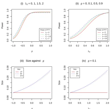
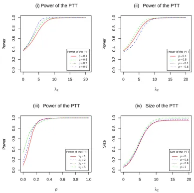
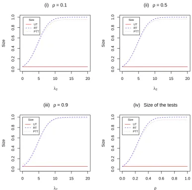
3.1 Power of the UT, RT and PTT against λ1 with ρ = 0.1 and λ2 =

0,1,1.5,2. . . 38 3.2 Size of the UT, RT and PTT against λ1 with λ2 = 0,1,1.5,2. . . 39

3.3 Power of the PTT and size against ρ and λ2. . . 40

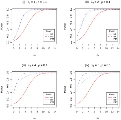
3.4 The power of the UT, RT and PTT against λ1 with ρ = 0.1 and

λ2 = 1, 2, 4, 5. . . 49

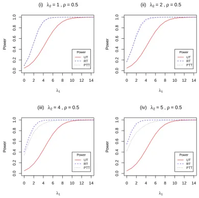
3.5 Power of the UT, RT and PTT against λ1 with ρ = 0.5 and λ2 =

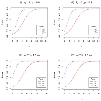
1, 2, 4, 5. . . 50 3.6 Power of the UT, RT and PTT against λ1 with ρ = 0.9 and λ2 =

1, 2, 4, 5. . . 51 3.7 Power and size of the PTT against λ2, and the power of the PTT

against ρ. . . 52 3.8 Size of the UT, RT and PTT against λ2 for selected ρ= 0.1, 0.5, 0.9,

and size against ρ. . . 53 3.9 Size of the UT, RT and PTT againstλ1 for selected values λ2 = 1,2,4,5. 54

4.1 Power of the tests againstϕ1for selected values ofρ, degrees of freedom

and noncentrality parameters. . . 72

4.2 Size of the tests against ϕ1 for selected values of ρ and ϕ2. . . . 73

5.1 Power function of the UT, RT and PTT against ζ1 for some selected

ρ, ζ2, degrees of freedom and noncentrality parameters. . . 87

5.2 Size of the UT, RT and PTT againstζ1 for some selectedρ,ζ2, degrees

of freedom and noncentrality parameters. . . 88

(12)

ρ, degrees of freedom and noncentrality parameters. . . 101 6.2 Size of the UT, RT and PTT against δ1 for some selected ρ and δ2. . 102

(13)

Chapter 1

Overview

1.1

Introduction

As a common practice, classical inferences about population parameters are always

drawn from the sample data alone. This applies to methods used in parameter

es-timation and hypothesis testing. Inferences about population parameters could be

improved using non-sample prior information (NSPI) from trusted sources (cf

Ban-croft, 1944). Such information, which is usually available from previous studies or

expert knowledge or experience of the researchers, is un-related to the sample data.

It is expected that the inclusion of NSPI in addition to the sample data improves

the quality of the estimator and the performance of the test. However, any NSPI

on the value of any parameter is likely to be uncertain (or unsure). In this case,

the information can be articulated in the form of a null hypothesis. An appropriate

statistical test on this null hypothesis will be useful to eliminate the uncertainty on

the suspected information. Then the outcome of the preliminary testing (pre-testing)

on the uncertain NSPI is used in the hypothesis testing or estimation. This approach

is likely to improve the quality of the estimator and the performance of the statistical

test (see Khan and Saleh, 2001; Saleh, 2006, p. 1; Yunus, 2010; Yunus and Khan,

2011a).

The NSPI can be classiﬁed as (i) unknown (unspeciﬁed) if NSPI on the value of

(14)

the parameter(s) is unavailable, (ii) known (certain or speciﬁed) if the exact value of

the parameter(s)is available, and (iii) uncertain if the suspected value is unsure (that

is, suspected to be a fixed quantity). For the three different scenarios, three different

estimators, namely the (i) unrestricted estimator (UE), (ii) restricted estimator (RE)

and (iii) preliminary test estimator (PTE) are deﬁned in the literature (see,e.g., Judge

and Bock, 1978; Saleh, 2006, p. 58). Khan (2003), and Khan and Hoque (2003)

provide the UE, RE, and PTE for diﬀerent linear models. For the testing purpose,

three diﬀerent statistical tests, namely the (i) unrestricted test (UT), (ii) restricted

test (RT) and (iii) pre-test test (PTT) are deﬁned along the same line as the three

diﬀerent estimators. The UE and UT use the sample data alone but the RE and RT

do not use the sample data alone. The PTE and PTT use both the NSPI and the

sample data. The PTE is a choice between the UE and RE, whereas the PTT is a

choice between the UT and RT. The choice depends on the outcome of the pre-testing

on the uncertain NSPI value. Note that by deﬁnition the test statistics of the PT and

UT are correlated but that of the PT and RT are uncorrelated, indeed independent.

Many authors have contributed to this area to the estimation of parameter(s) in

the presence of uncertain NSPI. Bancroft (1944, 1964, 1965) and Han and Bancroft

(1968) introduced a preliminary test estimation of parameters to estimate the

param-eters of a model with uncertain prior information. Later, Sclove et al. (1972), Stein

(1981), Maatta and Casella (1990), Bhoj and Ahsanullah (1994), Khan (2003, 2005,

2006a, 2006b, 2008), Khan and Saleh (1995, 1997, 2001, 2005, 2008), Khan et al.

(2002a, 2002b, 2005), Khan and Hoque (2003), and Saleh (2006, p. 55) covered

vari-ous work in the area of improved estimation using NSPI. But there is a very limited

number of studies on the testing of parameters in the presence of uncertain NSPI.

Although Tamura (1965), Saleh and Sen (1978, 1982), Yunus and Khan (2008, 2011a,

(15)

methods, the problem has not been addressed in the parametric context. Some

au-thors have studied the UE, RE and PTE for parametric cases (for instance Bechhofer

(1951), Bozivich et al. (1956), Bancroft (1964) and Saleh (2006)), but nor the tests.

The current research is to test the intercept parameter(s) when NSPI is available

on the slope parameter(s) of various linear models. The test statistics, their sampling

distributions, and power function of the tests are derived. Comparison of power

function of the tests are used to recommend a best test. In this thesis, we test

1. the intercept of thesimple regression model (SRM) when there is NSPI on the

slope,

2. the intercept vector of the multivariate simple regression model (MSRM) when

there is NSPI on the slope vector,

3. a subset of regression parameters of themultiple regression model (MRM) when

NSPI is available on another subset of the regression parameters, and

4. the equality of the intercepts for p(≥ 2) lines of the parallel regression model

(PRM) when there is NSPI on the slopes.

For each of the above four regression models, the following tasks are carried out:

1. derive the test statistics of the UT, RT and PTT for both known and unknown

variance,

2. derive the sampling distribution of the test statistics of the UT, RT and PTT,

and

3. derive and compare the power function and the size of the UT, RT and PTT.

For known variance, under a sequence of the alternative hypotheses, the sampling

(16)

follow normal distributions. However, the test statistic of the PTT follows a

bivari-ate normal distribution. For unknown variance, the sampling distribution of the test

statistics of the UT and RT of the simple regression model follow Student’st

distribu-tion but that of the PTT follows a correlated bivariate Student’s t distribution. For

the MSRM, MRM and PRM, the sampling distribution of the test statistics of the

UT and RT follow a univariate noncentral F distribution under alternative

hypoth-esis. However, the test statistic of the PTT follows a correlated bivariate noncentral

F (BNCF) distribution. For the above four regression models, there is a correlation

between the UT and PT but there is no correlation between the RT and PT. To

evaluate the power function of the PTT the probability integral of the bivariate

nor-mal, bivariate Student’s t and BNCF distributions are used. However, the bivariate

probability integrals of the above three distributions are very complicated.

Compu-tational formulas to evaluate the probability density function (pdf) and cumulative

distribution function (cdf) of the distributions are provided. The R package is used

for all computations and graphical analyses.

The computations of the power function of the PTT of the regression models

(MSRM, MRM and PRM) require the cdf of a correlated BNCF distribution. But

the correlated BNCF distribution is not available in the literature, and hence we

derive the pdf and cdf of the BNCF distribution. The pdf and cdf of the doubly

BNCF distribution are derived by mixing correlated bivariate noncentral chi-square

(BNCC) and central chi-square distributions. Whereas, the pdf and cdf of the singly

BNCF distribution are obtained by compounding the Poisson distribution with the

bivariate centralF (BCF) distribution. For the computation the probability integral

of the bivariate Student’s t distribution, we refer to the pdf of the multivariate t

distribution given by Kotz and Nadarajah (2004, p. 1).

(17)

and PTT are the size and power of the tests. A statistical test that has a minimum

size is preferable because it ensures a smaller probability of a type I error. Also, if

more than one statistical tests have the same power, the test that has a minimum

size is preferable. Furthermore, a test (or among the tests of the same size) that has

maximum power is preferred over any other tests because it guarantees the highest

probability of rejecting any false null hypothesis. A test that minimizes the size and

maximizes the power is preferred over any other tests. In reality, the size of a test

is ﬁxed, and then the choice of the best test is based on the criterion of maximum

power.

The study shows that the power of the RT is always higher than that of the UT

and PTT, and the power of the PTT lies between the power of the RT and UT. The

size of the UT is smaller than that of the RT and PTT. Among the three tests, the UT

has the lowest power and lowest size. In terms of power it is the worst and in terms

of size it is the best. The RT has maximum power and size. The PTT has smaller

size than the RT and the RT has larger power than the PTT. The PTT protects

against maximum size of the RT and minimum power of the UT. Thus, PTT attains

a reasonable dominance over the other two tests for all four regression models when

the suspected value of the parameter(s) suggested by the NSPI is not too far away

from its true value.

1.2

Main Contributions of the Thesis

The main contributions of the dissertation are as follow.

1. To use the uncertain NSPI in addition to the sample data to improve the

per-formance of the test.

(18)

• To test the intercept when NSPI is available on the value of the slope for

the simple regression model.

• To test the intercept when NSPI is available on the value of the slope for

the multivariate simple regression model.

• To test a subset of regression parameters when NSPI on another subset of

regression parameters is available for the multiple regression model.

• To test the equality of the two intercepts when NSPI on the equality of

the two slopes is available for the parallel regression model.

3. To determine the sampling distribution of the test statistics of the UT, RT and

PTT for the four diﬀerent regression models.

4. To derive the power functions of the UT, RT and PTT for the four diﬀerent

regression models.

5. To compare the power functions and the sizes of the UT, RT and PTT for the

four diﬀerent regression models.

6. To search for an optimum test that minimizes the size and maximizes the power

and recommend the best performing test with maximum power (for ﬁxed size).

For the SRM, we consider two cases for known and unknown variance, but for the

other models only the case of unknown variance/covariance is considered.

1.3

Thesis Outlines

The thesis consists of seven chapters, an overview is presented in Chapter 1.

Chap-ter 2 describes a liChap-terature review of previous works, some related distributions, the

bivariate noncentralF distribution and methodology of analysis. Testing of the

inter-cept for both cases of known and unknown variance by the UT, RT and PTT in the

(19)

in Chapter 3. Chapter 4 is devoted to testing the intercept by the UT, RT and PTT

for the multivariate simple regression model. Testing of a subset of regression

parame-ters by the UT, RT and PTT for the multiple regression model is provided in Chapter

5. Chapter 6 describes testing of the equality of the two intercepts by the UT, RT and

PTT for the parallel regression model. In each chapter, the study discusses the test

statistics, their distributions, power function of the tests and comparison of power of

the UT, RT and PTT. An illustrative example is given using simulated data. The

graphical representation of the power and size of the tests are also provided. Finally

the power function and size of the UT, RT and PTT are compared. The conclusion

(20)

Chapter 2

Literature Review, the Bivariate

Noncentral

F

Distribution and

Methodology of Analysis

2.1

Literature Review

2.1.1

The Preliminary Test Estimation

From Section 1.1, we see the use of prior information in the parameter estimation

or hypothesis test may improve the quality of the estimator or the performance of

the test. However, such a prior information is usually uncertain. This has warranted

the preliminary testing on the suspected value of the parameter(s) to remove the

uncertainty. The outcome of the pre-test is then incorporated into the procedure of

estimation or test on another parameter (cf Yunus, 2010).

Judge and Bock (1978), Khan and Saleh (2001), and Saleh (2006) have discussed

detail about the theory of pre-test in the area of parameter estimation including UE,

RE and PTE. There are a large number of published articles on the PTE given by

Saleh (2006); Khan (1998); Khan and Saleh (2001); Kabir and Khan (2009), among

others, whereas the idea of the PTE is introduced by Bancroft (1944, 1964). Later,

Bancroft (1965) implemented the idea of PTE in the ANOVA to study the eﬀect of

pre-testing on the estimation of variance.

(21)

To understand the concept of the PTE, we can refer to the problem of estimating

the population mean (µ) of any population based on a set of sample data when

it is apriori suspected that µ = µ0. Let X1,· · ·, Xn be a random sample from

N(µ, σ2_{). Then the sample mean} _X ₌ 1

n

∑n

i=1Xi is an unrestricted estimator (UE)

ofµ. Similarly the sample varianceS2 = _n₋1₁∑n_i₌₁(Xi−X

)2

is an unbiased estimator

of σ2. Based on the exclusive sample data, µU E =X. If the uncertain NSPI on µ is

given by µ0, then the restricted estimator (RE) of the mean is deﬁned as µRE =µ0.

Note µ0 does not depend on the sample data. To remove the uncertainty in the

suspected values of µ a statistical test is performed. In this case we test H0 :µ=µ0

versus Ha:µ̸=µ0 using the test statistic

t= X−µ0

S/√n

which follows a Student’s t distribution with (n−1) degrees of freedom. Then the

pre-test estimator (PTE) of µis deﬁned as

b

µP T E =µU EI(t0 ≥tα₂,n−1) +µREI(t0 < tα₂,n−1),

where α is the level of signiﬁcance and t0 is the observed value of the t statistic and

I(B) is the indicator function of the set B. Clearly PTE depends on the value of α

and it is either the UE or RE depending on the outcome of the pre-test on the NSPI.

The PTE can also be explained for the SRM,

Yi =β0+β1Xi +ei,

where the error variableei fori= 1,2,· · · , nare i.i.dN(0, σ2) (Wackerly et al., 2008,

p.581). If β0 and β1 be the unknown intercept and slope parameters, respectively,

with β1 =β10 (suspected), then the UE, RE and PTE are given as:

(i) the UE ofβ0 is the least square estimator (LSE) or maximum likelihood estimator

(MLE), βe0

U E

= Y −βe1X, where βe1 is the maximum likelihood estimator or,

equivalently, least square estimator of β1,X = 1_n

∑n

i=1Xi and Y = 1

n

∑n

(22)

(ii) the RE of β0 is βb0

RE

=Y −β10X, and

(iii) if the NSPI on β1 is uncertain, the uncertainty is removed by testing H0∗ :β1 =

β10 with the test statistic,

T2 = (βe1−β10)

2∑n

i=1(Xi−X) 2

SE(βe1)

,

where T2 _∼ _F

1,n−2 under H0∗. Based on the rejection or acceptance of H0∗, the PTE

of the intercept β0 is a choice between the UE and RE. The PTE of β0 is

e

β0

P T E

=βb0I(T2 < Fα,1,n−2) +βe0I(T2 ≥Fα,1,n−2),

where Fα,1,n−2 is the α-level upper critical value of a central F distribution with

(1, n−2) degrees of freedom. Hoque et al. (2009) explained that the PTE outperforms

the UE if the uncertain NSPI about the value of the slope is not too far from its true

value under the linex loss function. The PTE was also studied for other regression

models such as the MSRM (Sen and Saleh, 1979; Ahmed, 1992; Khan, 2005, 2006a)

and PRM ( Akritas et al., 1984; Lambert et al., 1985a; Khan, 2003). So far, a

lot of authors have covered various works in the area of improved estimation using

NSPI, but only a limited number of authors have studied the UT, RT and PTT

for parametric setup. However, studies of the PTE found that there is no uniform

domination among the UE, RE and PTE, and the PTE is an extreme choice between

the UE and RE. The question remains whether the UT, RT and PTT for parametric

regression models possesses the same kind of properties.

In the analysis of regression model, estimation of parameters and hypothesis

test-ing of parameters are two important aspects. Researchers are interested in estimattest-ing

both the slope and the intercept parameters. However the estimation of the intercept

parameter is more complicated than estimating the slope, as the former depends on

(23)

mod-els are assumed to be normal. For normal modmod-els, the maximum likelihood estimator

is identical to the least square estimator.

2.1.2

The Pre-test Test

There is a limited number of studies on the testing of parameters in the presence of

uncertain NSPI for the regression models. There are few articles found in the

liter-ature that use pre-test in the analysis of variance (Bechhofer, 1951; Bozivich et al.,

1956; Paull, 1950 among others). Ohtani and Toyoda (1985, 1986) considered the

problem of testing the linear hypothesis of regression coeﬃcients after pre-testing the

disturbance variance on the parametric linear regression model. Ohtani (1998), and

Ohtani and Giles (1993) extended the ideas related to this parametric problems. In

the same spirit, Lambert et al. (1985b) studied the performance of the UT, RT and

PTT on the parallelism model. Then, Yunus (2010), and Yunus and Khan (2011a,

2011b) studied the theory of pre-test in the area of hypothesis testing including the

UT, RT and PTT in the nonparametric context. So far, there is no study on the

performance of the power function of the PTT using the BNCF distribution for

mul-tivariate parametric regression models, namely the MSRM, MRM and PRM.

2.2

The Bivariate Central

F

Distribution

The BCF distribution is discussed in Krishnaiah (1964), Amos and Bulgren (1972),

Schuurmann et al. (1975), and El-Bassiouny and Jones (2009). Following Krishnaiah

(1964) for Xi =Fi ∼Fν1,ν2 with i= 1,2 and correlation coeﬃcientρ, the pdf and cdf

of the BCF distribution are deﬁned, respectively, as

f(x1, x2) = (

νν2/2

2 (1−ρ2)(ν1+ν2)/2

Γ(ν1/2)Γ(ν2/2) )

×∑∞

j=0 (

ρ2jΓ(ν1+ (ν2/2) + 2j)

j!Γ((ν1/2) +j) )

νν1+2j 1

×

(

(x1x2)(ν1/2)+j−1

[ν2(1−ρ2) +ν1(x1+x2)]ν1+(ν2/2)+2j )

(24)

P(X1 < d, X2 < d) = (

(1−ρ2₎ν1/2

Γ(ν1/2)Γ(ν2/2)

)_∑∞

j=0 (

ρ2j_Γ(_ν

1+ (ν2/2) + 2j)

j!Γ((ν1/2) +j) )

Lj,

(2.2.2)

where

Lj =

∫ h

0

∫ h

0

(x1x2)(ν1/2)+j−1dx1dx2

(1 +x1+x2)ν1+(ν2/2)+2j

,

with h = dν1

ν2(1−ρ2). An approximation to the value of the cdf of the BCF distribution

is also found in Amos and Bulgren (1972).

Krishnaiah (1964, 1965), and Krishnaiah and Armitage (1965) studied the

multi-variate central F distribution. Hewett and Bulgren (1971) studied about prediction

interval for failure times in certain life testing experiments using the multivariate

central F distribution. Later, Schuurmann et al. (1975) presented a statistical table

for the critical values of some selected multivariate central F distributions.

2.3

The Bivariate Noncentral

F

Distribution

Following Johnson et al. (1995, p. 480), we note that thedoublynoncentralF variable

with (ν1, ν2) degrees of freedom and noncentrality parameters λ1 andλ2 is deﬁned as

F_ν′′

1,ν2(λ1, λ2) =

χ′2

ν1(λ1)/ν1

χ′2

ν2(λ2)/ν2

, (2.3.1)

where the two noncentral chi-square distributions are independent. In many

applica-tions λ2 = 0, which arises when there is a central χ2 variable in the denominator of

F_ν′′₁_,ν₂. This is called a singly noncentral (or simply noncentral) F variable with (ν1,

ν2) degrees of freedom and noncentrality parameter λ1. The case for λ1 = 0, λ2 ̸= 0,

is not considered here, but note that

F_v′′

1,v2(0, λ2) =

1

F_v′₁_,v₂(λ2)

, E

[

F_v′

1,v2(λ1)

]

= v2(v1+λ1)

v1(v2−2)

, v2 >2, and

V ar

[

F_v′₁_,v₂(λ1) ]

= 2

(

v2

v1

)2(

(v1+λ1)2+ (v1+ 2λ1)(v2−2)

(v2−4)(v2−2)2

)

(25)

Moreover, Johnson et al. (1995, p. 499) described

G′′_ν₁_,ν₂(λ1, λ2) =

χ′_ν2₁(λ1)

χ′2

ν2(λ2)

(2.3.2)

as a mixture of Gν1+2j,ν2+2k distribution in proportion of

(

e−λ1/2(λ1 2 )j j! ) × (

e−λ2/2(λ2 2

)k

k!

)

,

representing product of two independent Poisson distributions. The details of the

probability density function and cumulative density function of G′′ are also found in Johnson et al. (1995, p. 500). Some discussions on the approximation of the

noncentral F distribution are found in Mudholkar et al. (1976). An approximation

to the multivariate noncentral F distribution is found in Tiku (1966).

2.3.1

The Singly Bivariate Noncentral

F

Distribution

Following Krishnaiah (1964) and Johnson et al. (1995, p. 499), for Xi =Fi ∼ Fν1,ν2

with i= 1,2, andR ∼ Pois(λ) the singly BNCF variable is given as

∞

∑

r=0 (

e−λ/2(λ

2 )r

r!

)

×Fνr,ν2, (2.3.3)

where νr = ν1 + 2r. Furthermore, the pdf of the singly BNCF distribution with

noncentrality parameter λ is given by the pdf

f(x1, x2, νr, ν2, λ) =

∞

∑

r=0 (

e−λ/2(λ

2 )r

r!

)

f1(x1, x2, νr, ν2), (2.3.4)

where f1(x1, x2, νr, ν2) is the pdf of a BCF distribution with νr and ν2 degrees of

freedom, that is,

f1(x1, x2, νr, ν2) = (

νν2/2

2 (1−ρ2)(νr+ν2)/2

Γ(νr/2)Γ(ν2/2)

) _∞

∑

j=0 (

ρ2jΓ(νr+ (ν2/2) + 2j)

j!Γ((νr/2) +j)

)

×(ννr+2j

r

) ( (x1x2)(νr/2)+j−1

[ν2(1−ρ2) +νr(x1+x2)]νr+(ν2/2)+2j )

.

(26)

Then the cdf of the singly BNCF distribution is deﬁned as

P(.) =P(X1 < d, X2 < d, νr, ν2, λ) =

∞

∑

r=0 (

e−λ/2(λ

2 )r

r!

)

×P2(X1 < d, X2 < d, νr, ν2),

(2.3.6)

where

P2(X1 < d, X2 < d, νr, ν2) = (

(1−ρ2)νr/2

Γ(νr/2)Γ(ν2/2) )

× ∞

∑

j=0 (

ρ2j_Γ(_ν

r+ (ν2/2) + 2j)

j!Γ((νr/2) +j)

)

Ljr

(2.3.7)

in which Ljr is deﬁned as

Ljr =

∫ hr

0 ∫ hr

0

(x1x2)(νr/2)+j−1dx1dx2

(1 +x1+x2)νr+(ν2/2)+2j

with hr = _ν₂₍₁dν₋r_ρ2₎.

For the computation of the value of the cdf of the singly BNCF distribution, R

codes are used. To make the computation easy, we rewrite the formula of the cdf of

(27)

P(.) =

∞

∑

r=0 (

e−λ/2(λ

2 )r

r!

) (

(1−ρ2)νr/2

Γ(νr/2)Γ(ν2/2) ) × ∞ ∑ j=0 (

ρ2j_Γ(_ν

r+ (ν2/2) + 2j)

j!Γ((νr/2) +j)

) Ljr = ∞ ∑ r=0 Tr [(

Γ(νr+ν2/2)

0!Γ(νr/2)

)

L0r+

(

ρ2Γ(νr+ν2/2 + 2)

1!Γ(νr/2 + 1)

)

L1r+· · ·

]

=

∞

∑

r=0

Tr[H0rL0r+H1rL1r+H2rL2r+· · ·]

=

∞

∑

r=0

TrH0rL0r+TrH1rL1r+TrH2rL2r+ · · · ·

= [T0H00L00+T0H10L10+T0H20L20 + · · · ·] +

[T1H01L01+T1H11L11+T1H21L21 + · · · ·] +

[T2H02L02+T2H12L12+T2H22L22 + · · · ·] + · · ·, (2.3.8)

where

Tr =

(

e−λ/2(λ₂)r r!

) (

(1−ρ2)νr/2

Γ(νr/2)Γ(ν2/2) )

,

H0r =

1Γ(νr+ (ν2/2))

0!Γ((νr/2))

, H1r =

ρ2Γ(νr+ (ν2/2) + 2)

1!Γ((νr/2) + 1)

,

H2r =

ρ4_Γ(_ν

r+ (ν2/2) + 4)

2!Γ((νr/2) + 2)

, · · · ,

and P0 is deﬁned as

P0 =

∞

∑

r=0

TrH0rL0r=T0H00L00+T1H01L01+T2H02L02+· · · ,for j = 0,

=

(

e−λ/2

0! ×

(1−ρ2₎ν1/2

Γ(ν1/2)Γ(ν2/2) ) (

1Γ(ν1+ν2/2)

0!Γ(ν1/2) )

L00 + (

e−λ/2(λ

2 )

1 ×

(1−ρ2₎ν1+2/2

Γ((ν1+ 2)/2)Γ(ν2/2) ) (

1Γ(ν1+ 2 + (ν2/2))

0!Γ((ν1+ 2)/2) )

L01

+· · · · . (2.3.9)

Similarly, we obtain the expressions for

P1 =

∞

∑

r=0

TrH1rL1r, P2 =

∞

∑

r=0

(28)

Finally we obtain

P(.) = P0+P1+P2+P3+ · · · ·=

∞

∑

j=0

Pj.

0.0 0.5 1.0 1.5 2.0 2.5 3.0

0.0 0.2 0.4 0.6 0.8 1.0

(i) ν1= 5, ν2= 20, ρ = 0.5

d

cdf

λ = 1

λ = 2

λ = 4

λ = 6

0.0 0.5 1.0 1.5 2.0 2.5 3.0

0.0 0.2 0.4 0.6 0.8 1.0

(ii) ν1= 20, ν2= 5, ρ = 0.5

d

cdf

λ = 1

λ = 2

λ = 4

λ = 6

0.0 0.5 1.0 1.5 2.0 2.5 3.0

0.0 0.2 0.4 0.6 0.8 1.0

(iii) ν1= 5, ν2= 20, ρ = −0.5

d

cdf

λ = 1

λ = 2

λ = 4

λ = 6

0.0 0.5 1.0 1.5 2.0 2.5 3.0

0.0 0.2 0.4 0.6 0.8 1.0

(iv) ν1= 20, ν2= 5, ρ = −0.5

d

cdf

λ = 1

λ = 2

λ = 4

[image:28.595.104.517.171.591.2]

λ = 6

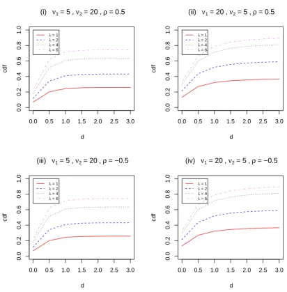
Figure 2.1: The cdf of the singly bivariate noncentral F distribution.

The graph of the cdf of the singly BNCF distributions is presented in Figure 2.1.

This ﬁgure shows that the value of the cdf of the singly BNCF distribution increases

as the value of any of the parameters, degrees of freedom ν1 (for ﬁxed ν2), λ, and d,

(29)

also depends on ρ. For both ρ < 0.5 and ρ > 0.5, the curves of the cdf of the singly

BNCF distribution are lower than that for ρ = 0.5. For ρ = −0.5 and ρ = 0.5,

the graph of the cdf of the singly BNCF distribution is identical. The R codes that

produce Figures 2.1 are provided in Appendix A.1.

2.3.2

The Doubly Bivariate Noncentral

F

Distribution

The doubly BNCF distribution is deﬁned by compounding the pdf of the BNCC

distribution of X1 and X2 with m degrees of freedom and noncentrality parameters

θ1 and θ2, and central chi-square distribution of Z with n degrees of freedom (see

Yunus and Khan, 2011c, and Amos and Bulgren, 1972). The pdf of the correlated

BNCC variables X1 and X2 is given by

g(x1, x2) =

∞

∑

j=0

∞

∑

r1=0 ∞

∑

r2=0

[

ρ2j(1−ρ2)m/2Γ(m/2 +j)]

×



 (x1)m/2+j+r1−1e− (x1) 2(1−ρ2)

[2(1−ρ2_)]m/2+j+r1_Γ(_m/_{2 +}_j ₊_r 1) ×

e−θ1/2₍_θ 1/2)r1

r1!

 

×



 (x2)m/2+j+r2−1e

− (x₂₎

2(1−ρ2)

[2(1−ρ2_)]m/2+j+r2Γ(m/2 +j +r 2)

× e−θ2/2(θ2/2)r2

r2!

 ,

(2.3.10)

and the pdf of a central chi-square variable Z with n degrees of freedom is

f(z) = z

(n/2)−1_e−z/2

2n/2_Γ(_n/₂₎ , z >0, (2.3.11)

whereZ is independent ofX1 andX2. Then using transformation of variable method

for multivariable case (see for instance, Wackerly et al. 2008, p. 325), we obtain the

joint pdf of y= [y1, y2]

′

and z variables as

(30)

where y1 = nx_mz1, y2 = nx_mz2 and the Jacobian of the transformation (x1, x2, z) →

(y1, y2, z), is given by

det.    ∂x1 ∂y1 ∂x1 ∂y2 ∂x1 ∂z ∂x2 ∂y1 ∂x2 ∂y2 ∂x2 ∂z ∂z ∂y1 ∂z ∂y2 ∂z ∂z  

=det.

 

m nz 0

m ny1

0 m_nz m_ny2

0 0 1

 = (_m nz )2 . (2.3.13)

Therefore, the joint pdf of y and z is given by

f(y, z) =

∞

∑

j=0

∞

∑

r1=0 ∞

∑

r2=0

[

ρ2j(1−ρ2)m/2Γ(m/2 +j)]

×



 (mny1z)

m/2+j+r1−1_e− (m_{n y}1z) 2(1−ρ2)

[2(1−ρ2_)]m/2+j+r1Γ(m/2 +j+r 1)

×e−θ1/2(θ1/2)r1

r1!

 

×



 (mny2z)

m/2+j+r2−1_e− (m_{n y}₂z) 2(1−ρ2)

[2(1−ρ2_)]m/2+j+r2Γ(m/2 +j+r 2)

×e−θ2/2(θ2/2)r2

r2!

 

× z(n/2)−1e−z/2

2n/2_Γ(_n/₂₎ ×

(_m

nz

)2

. (2.3.14)

Then the joint pdf of (Y1, Y2), where

Yi =

Xi/m

Z/n , for i = 1,2, (2.3.15)

is obtained as

f(y) = f(y1, y2) = ∫

z

(31)

that is,

f(y1, y2) =

(_m

n

)2[₍₁−_ρ2₎m/2

2n/2_Γ(_n/₂₎ ]

×∑∞

j=0

∞

∑

r1=0 ∞

∑

r2=0

[

ρ2jΓ(m/2 +j)] (e

−θ1/2₍_θ 1/2)r1

r1!

) (

e−θ2/2₍_θ 2/2)r2

r2!

)

×

[

(m_ny1)m/2+j+r1−1

[2(1−ρ2_)]m/2+j+r1Γ(m/2 +j+r 1)

]

×

[

(m_ny2)m/2+j+r2−1

[2(1−ρ2_)]m/2+j+r2Γ(m/2 +j+r 2)

]

×

∫ _∞

0

zm+n/2+2j+r1+r2−1_e−z/2 (₍_m/n₎_y

1 1−ρ2 +

(m/n)y₂

1−ρ2 +1

)

dz

=

(_m

n

)2[₍₁−_ρ2₎m/2

2n/2_Γ(_n/₂₎ ] × ∞ ∑ j=0 ∞ ∑

r1=0 ∞

∑

r2=0

[

ρ2jΓ(m/2 +j)] (e

−θ1/2₍_θ 1/2)r1

r1!

) (

e−θ2/2₍_θ 2/2)r2

r2!

)

×

(_m

n

)m+2j+r1+r2−2[

ym/2+j+r1−1

1 y

m/2+j+r2−1 2

]

[2(1−ρ2_)]m+2j+r1+r2_Γ(_m/_{2 +}_j₊_r

1)Γ(m/2 +j+r2)

×

(

2

wy

)qrj

Γ(qrj)

=

(_m

n

)m[₍₁−_ρ2₎m+₂n

Γ(n/2)

] _∞

∑

j=0

∞

∑

r1=0 ∞

∑

r2=0

[

ρ2j

(_m

n

)2j

Γ(m/2 +j)

]

×

[(

e−θ1/2₍_θ 1/2)r1

r1!

) ( (m

n

)r1

Γ(m/2 +j+r1) ) (

ym/2+j+r1−1 1

)]

×

[(

e−θ2/2₍_θ 2/2)r2

r2!

) ( (_m

n

)r2

Γ(m/2 +j+r2) ) (

ym/2+j+r2−1 2

)]

× Γ(qrj)

[

(1−ρ2) + m

ny1+ m

ny2

]₋(qrj)

, (2.3.17)

where wy = (m/n₁₋_ρ)2y1 +

(m/n)y2

1−ρ2 + 1 and qrj = m+n/2 + 2j +r1+r2. The cdf of the

doubly BNCF distribution is then deﬁned as

P(Y1 < a, Y2 < b) =

∫ a

0

∫ b

0

f(y1, y2)dy1dy2, (2.3.18)

(32)

The above cdf can be expressed as

P(Y1 ≤a, Y2 ≤b) =

∫ _∞

0

f(z)

∫ bmy n 0 ∫ amy n 0

g(x1, x2)dx1dx2dz, (2.3.19)

whereg(x1, x2) is the pdf of a BNCC distribution which is given in Equation (2.3.10),

f(z) is the pdf of the central chi-square variable which is given in Equation (2.3.11),

and Yi fori= 1,2, are given in Equation (2.3.15).

Equation (2.3.19) can be written as

P(Y1 ≤a, Y2 ≤b) = (1−ρ2)

m

2 ∞

∑

r1=0 ∞

∑

r2=0 ∞

∑

j=0

(m₂)j

j! ρ

2j_I

2( ˜αj,˜c, β)

×e−θ1/2(θ1/2)r1

r1!

e−θ2/2₍_θ 2/2)r2

r2!

, (2.3.20)

where

I2( ˜αj,˜c, β) =

∫ _∞

0

e−z_zβ−1

Γ(β)

γ(α1, c1z)

Γ(α1)

γ(α2, c2z)

Γ(α2)

dz (2.3.21)

and

β = n

2, c˜=

(

am n(₁−_ρ2₎,

bm n(₁−_ρ2₎

)

, α˜j =

(_m

2 +j+r1,

m

2 +j +r2

)

.

(2.3.22)

Here, γ(α, x) =∫₀xe−ttα−1dt, and Γ(α) = ∫₀∞e−ttα−1dt.

Amos and Bulgren (1972) used various representations ofγ(α1, c1z) andγ(α2, c2z)

and derived the series form of I2( ˜αj,˜c, β) in terms of regularized beta functions. In

this paper we use the I2 as given by Amos and Bulgren (1972), that is,

I2( ˜αj,c, β˜ ) = Iu(α1, β)−

(1−u)β

α1

Γ(β+α1)

Γ(β)Γ(α1)

× ∞

∑

r=0

(β+α1)r

(1 +α1)r

ur+α1_I

1−y(r+β+α1, α2), (2.3.23)

with

(33)

and

∫ _∞

0

e−z_zβ−1

Γ(β)

γ(α, cz)

Γ(α) dz = Iz(α, β) and

∫ _∞

0

e−zzβ−1

Γ(β)

Γ(α, cz)

Γ(α) dz = I1−z(β, α)

are the regularized beta functions, with α > 0, β > 0, x = c/(1 +c), and 1−x =

1/(1 +c).

The inﬁnite series is truncated aftert1+ 1, t2+ 1 andt3+ 1 terms and thus giving

a bound on the truncation error, say rt. For any ﬁnite a and b,

kj = (1−ρ2)

m

2 ∞

∑

j=0

(m₂)j

j! ρ

2j_I

2( ˆαj,c, βˆ ),

the mass of a bivariate central F distribution and

sri =

e−θi/2₍_θ

i/2)ri

ri!

, i= 1,2,

the mass of a Poisson distribution,

rt1,t2,t3 = ∞

∑

j=t1+1 ∞

∑

r1=t2+1 ∞

∑

r2=t3+1

kjsr1sr2 = 1−

t1

∑

i=0

t2

∑

r1=0

t3

∑

r2=0

kjsr1sr2.

The stopping value of t1, t2 and t3 that are used depends on machine and software

precision. In practice, rt is computed successively and iteration stops when rt−1 =rt

(34)

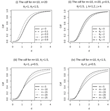
0 1 2 3 4 0.0 0.2 0.4 0.6 0.8 1.0 d Cdf

(i) The cdf for m=10, n=20

θ1=1, θ2=1.5,

ρ =0

ρ =0.1

ρ =0.3

ρ =0.5

ρ =0.9

0 1 2 3 4

0.0 0.2 0.4 0.6 0.8 1.0 d Cdf

(ii) The cdf for m=10, n=20, ρ=0.5,

θj=1.5, j, k=1,2, j≠k

θk=0 θk=1 θk=2 θk=3 θk=4

0 1 2 3 4

0.0 0.2 0.4 0.6 0.8 1.0 d Cdf

(iii) The cdf for m=10, θ1=1.5,

θ2=1, ρ=0.5,

n=5 n=10 n=15 n=20 n=25

0 1 2 3 4

0.0 0.2 0.4 0.6 0.8 1.0 d Cdf

(iv) The cdf for n=10, θ1=1.5,

θ2=1, ρ=0.5,

[image:34.595.130.491.70.433.2]

m=5 m=10 m=15 m=20 m=25

Figure 2.2: The cdf of thedoubly bivariate noncentral F distribution.

The values of the cdf of thedoubly BNCF distribution are computed for arbitrary

degrees of freedom (m, n), noncentrality parameter (θ1, θ2), and correlation coeﬃcient

(ρ). The graph of the cdf of the doubly BNCF distribution is presented in Figure

2.2. The cdf of the BNCF distribution is computed using Equation (2.3.20). Figure

2.2 shows the cdf of the doubly BNCF distribution depends on the values of the

noncentrality parameters (θ1,θ2), degrees of freedom (m, n), correlation coeﬃcient (ρ)

and upper limit (d). For the Figure 2.2, we observe that the shape of the curve of the

cdf is sigmoid. Also, the value of the cdf approaches 1 quicker for a larger correlation

(35)

and larger degrees of freedom (m, n) (see Figures 2.2(iii) and 2.2(iv)).

The R codes used to plot the cdf of the BNCF distribution in Figure 2.2 are

provided in Appendix A.2.

2.4

The Methodology of Analysis

For each of the four regression models, we deﬁne the test statistic for the UT, RT

and PTT, derive the sampling distribution of the test statistics and power function

of the tests, present a simulation example, compare the power function and size of

the tests, and recommend a test that minimizes the size and maximizes the power.

2.4.1

The UT, RT, PT and PTT

Consider the problem of testing intercept in the SRM, H0 :β0 = β00 (a ﬁxed value)

againstHa:β0 > β00, when there is uncertain NSPI available on the value slope (β1).

In this situation, three diﬀerent scenarios on β1 are considered, namely unspeciﬁed,

specified and uncertain. We then define three different statistical tests, namely, the

(i) unrestricted test (UT), (ii) restricted test (RT) and (iii) pre-test test (PTT). For

the UT, let ϕU T _{be the test function for testing} _H

0. For the RT, let ϕRT be the

test function for testing H0. Whereas for the PTT, let ϕP T T be the test function for

testing H0 following a pre-test (PT) on the slope. Then, for the PT, let ϕP T be the

test function for testing H₀∗ : β1 = β10 against Ha∗ : β1 > β10, and it is essential for

the PTT on β0. The PTT is a choice between the UT and RT. If H0∗ is rejected in

PT, then the UT is used to test H0, otherwise the RT is used. The details on the

(36)

The Unrestricted Test (UT)

If the slope (β1) is unspeciﬁed, the test functions is ϕU T. Let, TU T be test statistic

to test H0, then chose a value of α1 (0< α1 <1) such that,

P [TU T > ℓU T_n,α

1 |H0 :β0 =β00

]

=α1, (2.4.1)

where ℓU T

n,α1 is the critical value of T

U T _{at the} _α

1 level of signiﬁcance. If ταi is the

upper 100αi quantile and Φ(.) is the cumulative distribution function of the standard

normal distribution, then

Φ(ταi) = 1−αi, (2.4.2)

where 0< αi <1, i= 1, 2, 3. Thus, 1−α1 can be written as

1−α1 =P [

TU T ≤ℓU T_n,α

1

]

. (2.4.3)

Hence, for the test functionϕU T ₌_I₍_TU T _{> ℓ}U T

n,α1), the power function of UT becomes

πU T(β0) = E(ϕU T |β0) =P(TU T > ℓU Tn,α1 |β0). (2.4.4)

The Restricted Test (RT)

If β1 =β10 (speciﬁed), then the test function is ϕRT. Let the proposed test statistic

to test H0 :β0 =β00 against Ha :β0 > β00, whenβ1 =β10 be TRT. Then, we ﬁnd

P[TRT > ℓRT_n,α₂ |H0 :β0 =β00, β1 =β10 ]

=α2, (2.4.5)

where ℓRT_n,α₂ is the critical value ofTRT at the α2 level of signiﬁcance. We then obtain

1−α2 =P [

TRT ≤ℓRT_n,α

2

]

. (2.4.6)

Thus, for the test function ϕRT ₌_I₍_TRT _{> ℓ}RT

n,α2), the power function of RT is

(37)

The Pre-test (PT)

Ifβ1 is uncertain, letϕP T be the test function for testing the hypothesisH0∗ :β1 =β10

against H_a∗ :β1 > β10. Let the proposed test statistic be TP T. Under H0∗, we ﬁnd

P [TP T > ℓP T_n,α₃ |H₀∗ :β1 =β10 ]

=α3, (2.4.8)

Similarly, we ﬁnd

1−α3 =P [

TP T ≤ℓP T_n,α

3

]

, (2.4.9)

whereℓP T

n,α3 is the critical value of theT

P T _{at the}_α

3 level of signiﬁcance. Furthermore,

for the test function ϕP T ₌_I₍_TP T _{> ℓ}P T

n,α3), the power function of the PT is given by

πP T(β0) = E(ϕP T |β0) =P(TP T > ℓP Tn,α3 |β0). (2.4.10)

The Pre-test Test (PTT)

To formulate a test function of the PTT for testing the hypothesis H0 : β0 = β00

against Ha : β0 > β00 after pre-testing (PT) on the suspected value of the slope, we

write ϕP T T _as

ϕP T T =I[(TP T ≤ℓP T_n,α₃, TRT > ℓRT_n,α₂) or (TPT > ℓPT_n_,α₃,TUT > ℓUT_n_,α₁)]. (2.4.11)

Then the power function of the PTT, denoted by πP T T₍_β

0) =E(ϕP T T |β0), is given

as

πP T T(β0) =P (

TP T ≤ℓP T_n,α

3, T

RT _{> ℓ}RT n,α2 |β0

)

+P (TP T > ℓP T_n,α

3, T

U T _{> ℓ}U T n,α1 |β0

)

.

(2.4.12)

2.4.2

The Power Function and Size of the Tests

The goodness of a test is measured by the probability of the type I error (α) and the

probability of the type II error (β). Whereas, to evaluate the performance of a test,

(38)

test will lead to the rejection of the H0 : θ = θ0 against an alternative hypotheses

Ha : θ ̸= θ0 when the actual parameter value is diﬀerent from θ0. Generally, the

power of a test can be written as

π(θ) =P(Wis inRRwhen the parameter value isθ),

where W is the value of the test statistic andRR is the rejection region for the test.

With regard to the rejection region, so

π(θa) = P(rejecting H0whenθ =θa),

where θa is a value of θ under Ha. Note that a good test ideally has power near 1

under Ha and near 0 under H0 (Casella and Berger, 2002, p. 383).

The following example is to describe the power function and size of a test. Let

Xi, i = 1,2, ..., n be independent and each of them follows a Bernoulli distribution

with parameter θ. Then for n = 10 trials, Y = ∑n_j₌₁=10Xj follows a binomial

dis-tribution with n = 10 and p = θ, and denoted as Y ∼ Bin(n, θ). We want to test

H0 : θ = 0.5 against Ha : θ = 0.4, with RR = {(x1,· · ·, x10) : Y ≤ 3}. The power

function of the test deﬁned by RR (under Ha) is given as

π(θ) = P(Reject H0 |θ) = 3 ∑

y=0 (

10

y

)

θy(1−θ)10−y

= (1−θ)7(84θ3+ 28θ2+ 7θ+ 1). (2.4.13)

The size of the test is the value of power function under H0, that is,

α = P(Type I error) = π(θ |H0 :θ=θ0) = P(Reject H0 |H0 is true)

= P(Y ≤3|θ = 0.5) = (1−θ)7[84(θ)3+ 28(θ)2+ 7(θ) + 1]|H0 :θ = 0.5

= (1−0.5)7(84(0.5)3+ 28(0.5)2+ 7(0.5) + 1) = 0.1719 (2.4.14)

(39)

is true) is given by

β = P(Type II error) = P(Accept H0 |Ha is true)

= P(Y >3|θ = 0.4)

= 1−((1−θ)7(84(θ)3+ 28(θ)2+ 7(θ) + 1))|Ha=θ=0.4= 0.618 (2.4.15)

Generally, the power function of the UT, RT, PT and PTT are produced using

Equa-tions (2.4.4), (2.4.7), (2.4.10) and (2.4.12). For the simulation example, the power

(π(θ)), size (α) and probability of type II error (β) are produced using Equations

(2.4.13), (2.4.14) and (2.4.15). The above computation in Equations (2.4.13) and

(2.4.14) proves that the size and power of the test are obtained from the power

func-tion of the test (see Pinto et al., 2003; Saleh and Sen, 1982, 1983). The size (α)

is commonly chosen and set as the probability of type I error (see Wackerly et al.,

2008, p. 491, and De Veaux et al., 2009, p. 544). The size of the test as the nominal

value under the null hypothesis is constant and the power of the test depends on the

parameter θ. Furthermore, a test that maximizes the power function and minimize

Test of hypotheses for linear regression models with non-sample prior information