Faculty of Health, Engineering and Sciences
Statistical Methodology for Regression Model
with Measurement Error
A thesis submitted by
Anwar A. Mohamad Saqr
B.Sci., M.Sci.
in fulfilment of the requirements for the degree of
Doctor of Philosophy
Abstract
This thesis primarily deals with the estimation of the slope parameter of the simple linear regression model in the presence of measurement errors (ME) or error-in-variables in both the explanatory and response variables. It is a
very old and difficult problem which has been considered by a host of authors since the third quarter of the nineteenth century. The ME poses a serious problem in fitting the regression line, as it directly impacts on estimators
and their standard error (see eg Fuller, 2006, p. 3). The standard linear regression methods, including the least squares or maximum likelihood, work when the explanatory variable is measured without error. But in practice,
there are many situations where the variables can only be measured with ME. For example, data on the medical variables such as blood pressure and blood chemistries, agricultural variables such as soil nitrogen and rainfall etc
with ME.
The ME model is divided into two general classifications, (i) functional model if the explanatory (ξ) is a unknown constant, and (ii) structural model ifξ is independent and identically distributed random variable (cf Kendall, 1950,
1952). The most important characteristic of the normal structural model is that the parameters are not identifiable without prior information about the error variances as the ratio of error variances (λ) (see Cheng and Van Nees, 1999, p. 6). However, the non-normal structural model is identifiable with-out any prior information. The normal and non-normal structural models with ME in both response and explanatory variables are considered in this
research.
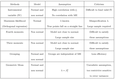
There are a number of commonly used methods to estimate the slope param-eter of the ME model. None of these methods solves the estimation problem in varying situations. A summary of the well known methods is provided in
Table 1.
The first two chapters of this thesis cover an introduction to the ME problem, background, and motivation of the study. From Chapter 3 we provide a new methodology to fit the regression line using the reflectionof the explanatory
iii
Table 1: A summary of commonly used methods to handle the ME model
problem
Methods Model Assumption Criticism
Instrumental Normal and High correlation withξ. Difficult to fond valid IV
variable (IV) non normal No correlation with ME
Maximum likelihood Normal λknown Misspecificationλ.
(Orthogonal regression) True points fall on a straight line Large sample required
Fourth moments Non normal Model not close to normal. Difficult to satisfy
Large sample size these assumptions
Three moments Non normal Model not close to normal. Difficult to satisfy
Large sample size these assumptions
Grouping Normal and Groups are independent of ME Less efficiency
non normal
Geometric Mean Normal and Unrealistic assumption,
non normal λ=β12 too restrictive sensitive to error variances
to compare the new estimators and the relevant existing estimators under
different conditions.
One of the most commonly used methods to deal with the ME model is the instrumental variable (IV) method. But it is difficult to find valid IV that is highly correlated to the explanatory but uncorrelated with the error term.
this method is demonstrated both analytically and via numerical as well as
graphical illustrations under certain assumptions.
In Chapter 5, a commonly used method to deal with the normal structural model, namely the orthogonal regression (OR) (which is the same the maxi-mum likelihood solution whenλ= 1) method under the assumption of known
λ is discussed. But the OR method does not work well (inconsistent) if λ
is misspecified and/or the sample size is small. We provide an alternative method based on the reflection method (RM) of estimation for
measure-ment error model. The RM uses a new transformed explanatory variable which is derived from the reflection formula. This method is equivalent or asymptotically equivalent to the orthogonal regression method, and nearly
asymptotically unbiased and efficient under the assumption that λ is equal to one and the sample size is large. If λ is misspecified the RM method is better than the OR method under the MAE criterion even if the sample size
is small.
Chapter 6 considers the Wald method (two grouping method) which is still widely used, in spite of increasing criticism on the efficiency of the estimator. To address this problem, we introduce a new grouping method based on
v
the reflection of the explanatory variable. The method recommends different
grouping criteria depending on the value of λ to be one or more/less than one. The RG method significantly increases the efficiency of Wald method, and it is more precise than the other competing methods and works well for
different sample sizes and for different values ofλ. Moreover, the RG method also removes the shortcomings of the maximum likelihood method whenλ is misspecified and sample size is small.
The geometric mean (GM) regression is covered in Chapter 7. The GM
method is widely used in many disciplines including medical, pharmacol-ogy, astrometry, oceanography, and fisheries researches etc. This method is known by many names such as reduced major axis, standardized major
axis, line of organic correlation etc. We introduce a new estimator of the slope parameter when both variables are subject to ME. The weighted ge-ometric mean (WGM) estimator is constructed based on the reflection and
the mathematical relationship between the vertical and orthogonal distances of the observed points and the regression line of the manifest model. The WGM estimator possesses better statistical properties than the geometric
mean estimator, and OLS-bisector estimator. The WGM estimator is stable and work well for different values of λ and for different sample sizes.
es-timators by simulation studies. The computer package Matlab is used for
all computations and preparation of graphs. Based on the asymptotic con-sistency and MAE criteria the proposed reflection estimators perform better than the existing estimators, in some cases, even the standard assumption
on λ and sample size are violated.
Certification of Dissertation
I certify that the ideas, designs and experimental work, results, analyses and
conclusions set out in this dissertation are entirely my own effort, except where otherwise indicated and acknowledged.
I further certify that the work is original and has not been previously
submit-ted for assessment in any other course or institution, except where specifically stated.
Signature of Candidate
Signature of Principal Supervisor
Acknowledgments
My first and foremost thanks to ALLAH for the opportunities that He has given to me throughout my life, especially those that have brought me to the position of finishing this thesis. I would like to express my thankful-ness and gratitude to my principal supervisor Professor Shahjahan Khan for his invaluable assistance, support, patience and guidance during the period of my research, without his knowledge and assistance this study would not have been successful. My special thanks and gratitude go to my associate supervisor Dr Trevor Langlands for his advice, support, constructive feed-back and invaluable assistance. I would like to thank all the staff in the faculty of health, engineering and sciences specially the staff of the school of agricultural, computational and environmental sciences and the library for providing a very good scientific environment for statistical research.
This thesis is dedicated to the souls of my mother and father (may ALLAH
bless them with Jannah), that I wish them to be alive to see what I have
achieved and to share my happiness for completing this thesis, who always
supported, encouraged and directed me for higher education.
Contents
Abstract i
Acknowledgments viii
List of Figures xv
List of Tables xviii
List of Notations xx
Chapter 1 Introduction 1
1.1 Introduction . . . 1
1.3 Outline of the Thesis . . . 10
Chapter 2 Historical background of measurement error mod-els 17 2.1 Introduction . . . 17
2.2 Major Axis Regression (Orthogonal) . . . 18
2.3 Deming Regression Technique . . . 20
2.4 Grouping Method . . . 22
2.5 Reduced Major Axis . . . 27
2.6 Moments estimators . . . 30
2.6.1 Estimators based on the first and second moments . . . 30
2.6.2 The method of higher-order moments . . . 38
2.6.3 Estimation with cumulants . . . 46
2.7 Instrumental Variables . . . 50
2.8 Method based on ranks . . . 53
CONTENTS xi
2.10 Structural equation modelling . . . 60
2.11 Other contributions . . . 62
Chapter 3 The reflection approach to measurement error model 64 3.1 Introduction . . . 64
3.2 Methodology . . . 65
3.3 Residuals analysis by reflection technique . . . 66
3.3.1 An alternative proof . . . 70
3.4 Advantages of using reflection . . . 72
3.5 Concluding remarks . . . 88
Chapter 4 Instrumental variable estimator for measurement error model 89 4.1 Introduction . . . 89
4.2 Measurement error models . . . 90
4.3.1 Instrumental variable (IV) estimator . . . 94
4.4 Proposed new IV estimator . . . 96
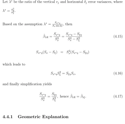
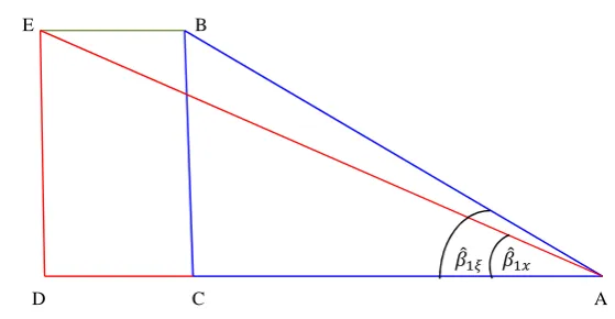
4.4.1 Geometric Explanation . . . 99
4.5 Some properties and relationships . . . 101
4.6 Illustration . . . 103
4.6.1 Yield of Corn Data . . . 103
4.6.2 Hen Pheasants Data . . . 106
4.7 Concluding Remarks . . . 109
Chapter 5 Reflection method of estimation for measurement error models 111 5.1 Introduction . . . 111
5.2 Orthogonal regression method . . . 114
5.3 Proposed reflection method of estimation . . . 116
5.3.1 Geometric explanation . . . 118
CONTENTS xiii
5.5 Simulation studies . . . 126
5.6 Concluding remarks . . . 131
Chapter 6 Reflection in grouping method estimation 133 6.1 Introduction . . . 133
6.2 Wald’s grouping method . . . 134
6.3 Proposed reflection grouping method . . . 138
6.3.1 Propose modifications to Wald’s method . . . 146
6.3.2 Example . . . 149
6.4 Simulation studies . . . 150
6.4.1 First study: Non-normal distributions of ξ . . . 151
6.4.2 Second study: Normal distributions of ξ . . . 154
6.5 Concluding remarks . . . 158
7.2 Relationship between the vertical and orthogonal distances . 162
7.2.1 Fitted line case . . . 164
7.2.2 Unfitted line case . . . 166
7.3 Geometric mean estimator . . . 168
7.4 Alternative view on the geometric mean estimator . . . 170
7.5 Proposed estimator . . . 171
7.6 Simulation studies . . . 172
7.7 Concluding remarks . . . 176
Chapter 8 Conclusions 178 8.1 Conclusions and Summary . . . 179
Bibliography 182
List of Figures
3.1 Graph of a reflection point about the OLS regression line of y
onx. . . 71
4.1 Graph representing the sum of squares and products in the
presence of measurement error in the explanatory variable. . . 101
4.2 Graph representing the sum of squares and products when the measurement error in the explanatory variable is ’treated’ by reflection. . . 102
5.1 Graph of the sum of squares and products of the latent and
5.2 (a) Graph of the slope estimated and (b) Graph of MAE of
the RM, OR, and OLS estimators ofβ1, when λ= 1 is correct and small sample sizes 10< n <30. . . 130 5.3 (a) Graph of the slope estimated and (b) Graph of MAE of
the RM, OR, and OLS estimators for β1, when λ(= 1.44) is incorrect and larger sample sizes 10< n <120. . . 131
6.1 Graph of the estimated slope (a) and the mean absolute error (b) for five different estimators whenλ = 1, and β1 = 1. . . 151 6.2 Graph of the estimated slope (a) and the mean absolute error
(b) for five different estimators whenλ >1, and β1 = 1. . . 152 6.3 Graph of the estimated slope and the mean absolute error for
five different estimators whenλ <1, and β1 = 1. . . 153 6.4 Graphs of the estimated slope (a) and the mean absolute error
(b) for four different estimators RG1, M L, W, and OLS for case I. . . 155
6.5 Graphs of the estimated slope (a) and the mean absolute error
LIST OF FIGURES xvii
6.6 Graphs of the estimated slope and the mean absolute error for
four different estimators RG3, M L, W, and OLS for case III. 157
7.1 Graph of two orthogonal distances (AB=Od, andAD =Ox) between the observed point and the fitted and unfitted lines. . 163
7.2 Graph of three estimators of the slope, and the mean absolute error when β0 = 20, β1 = 0.55 and 0.08≤λ≤100. . . 173 7.3 Graph of three estimators of the slope, and the mean absolute
error when β0 = 27, β1 =−0.75 and 0.08≤λ≤100. . . . 174 7.4 Graph of three estimators of the slope, and the mean absolute
List of Tables
1 A summary of commonly used methods to handle the ME
model problem . . . iii
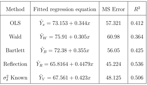
4.1 Fitted regression models for the corn yield data . . . 104
4.2 Fitted regression models for the Hen peasants data . . . 107
5.1 The simulated mean of five different estimators and the MAE
when β1 = 1, β0 = 0, n = 100. . . 128 5.2 The simulated mean of five different estimators with the MAE
when β1 = 2, β0 = 0, n = 100. . . 128
LIST OF TABLES xix
7.1 Simulated mean values of the estimated slope and the mean
List of Notations
ξj Unobserved explanatory variable (latent variable).
ηj Unobserved response variable (latent variable).
xj Observed explanatory variable (manifest variable).
yj Observed response variable (manifest variable).
x∗j Reflection of the observed explanatory variable.
y∗j Reflection of the observed response variable (manifest variable).
δj Measurement error in the explanatory variable.
ϵj Measurement error in the response variable.
ej Equation error in the true model.
vj Equation error in the Measurement Error model.
ψ Reflection angle about the unfitted regression line (by manifest variables).
Chapter 1
Introduction
1.1
Introduction
Regression analysis forms an important part of the statistical tools for inves-tigating the relationships between variables. For example, regression analysis may be used to investigate whether there is a relationship between the
num-ber of road accidents and the age of the driver. Linear regression is a com-mon statistical data analysis technique in the fields of medical, agricultural, chemical, physical and economic studies (Gillard and Iles, 2009; Warton et
moisture level, is likely to involve measurement error (Anderson 1984). The
ordinary least squares (OLS) estimator of the regression parameters is inap-propriate in the presence of measurement error (cf Fuller, 2006, p. 3). As a result, in real life, measurement error causes a serious problem as it directly
impacts on estimators and their standard error. It is well known that the measurement error in the response variable is not as serious as it is in the explanatory variable. The error in the response variable can be absorbed in
the error term of the model; however, the error in the explanatory variable causes various problems, and needs to be handled appropriately (Madansky 1959).
The measurement error (ME) or error-in-variables is a real problem and it
has been considered by a host of authors since the late nineteenth century (Gillard, 2010). Adcock (1877, 1878) discussed the problem in the context of least squares method. Pearson (1901) suggested some estimators based on
Adcock’s work. The problem has been seriously considered by researchers from the last century. Wald (1940), Bartlet (1949), Durbin (1954), and Riggs et al. (1978), considered fitting the regression line when both variables are
subject to error. Berkson (1950) noted that the error in the explanatory variable leads to bias in the estimated parameters of the regression line, regardless of the data being a random sample or the population. Burr (1988)
1.1 Introduction 3
Freedman et al. (2004) suggested a moment method to deal with error in the
explanatory variable. The problem of error in both explanatory and response variables was considered by Madansky (1959) and Halperin (1961).
Degracie and Fuller (1972) considered estimation of the slope and covariance when the variable is measured with error. Grubbs (1973) discussed error of
measurement, precision and the statistical inference. Aigner (1973) consid-ered regression with a binary variables subject to the error of observation. Florens et al. (1974) considered Bayesian inference in error-in-variables
mod-els. Schneeweiss (1976) proposed consistent estimation of a regression with error in the variables. Bhargava (1977) introduced maximum likelihood esti-mation in a multivariate error-in-variables regression model with an unknown
error covariance matrix. Garber and Klepper (1980) extended the classical normal error-in-variables model. Prentice (1982) dealt with covariant mea-surement error and parameters estimation.
Amemiya et al. (1984) proposed estimation of the multivariate
error-in-variables model with estimated error covariance matrix. Klepper and Leamer (1984) provided consistent sets of estimates for regression with error in all variables. Stefanski and Carroll (1985) discussed covariant measurement
linear model. Bekker (1986) provided comments on the identification issues
in the measurement error model. Schafer (1986) combined information on the measurement error model. Carroll and Ruppert (1996) discussed the use and misuse of orthogonal regression in the measurement error model.
Fuller (2006) covered various aspects of the measurement error model and related inferences. Carroll et al. (2006) summarized much of what is known about the consequences of measurement error for estimating the linear
re-gression parameters. Recently McCartin (2010) has introduced a new con-cept of oblique linear least squares approximation. This thesis introduces a new methodology of fitting a straight regression line when both response
and explanatory variables are subject to error. This has not been discussed previously in the literature of measurement error.
It is well known that the fitting of a straight line to bivariate data (ξ, η) is a common procedure and widely used in analysis of linear relationships.
This procedure works under the standard linear regression theory where the explanatory variable is measured without error. The response variable η
depends on the explanatory variableξ according to the usual additive model
ηj =β0+β1ξj+ej, j = 1,2,· · · , n, (1.1)
where ej is a random error representing the intrinsic scatter in η about the
1.1 Introduction 5
The main goal here is to estimate the parameters β0 and β1 of the model (1.1). One of the common techniques to estimate these parameters involves minimising the function of the random error term ej. This technique, called
the least squares theory, suggests minimising the sum of the squared error
components, and was introduced by Carl Freidrich Gauss (1777-1855) and Adrien Marie Legendre (1752-1833). Here the regression line of η on ξ is obtained by minimising the sum of squares of the vertical distances from the
points (ξj, ηj) to the regression line which is given by the estimated equation
model ˆηj = ˆβ0+ ˆβ1ξj. This is given by n
∑
j=1
e2j =
n ∑
j=1
(ηj −β0−β1ξj)2,
where the least squares estimators of the parameters β0 and β1 can be ob-tained by differentiating∑nj=1e2
j with respect to each of the parameters, and
solving the equations which arise after setting the derivatives to zero to find
ˆ
β1 =
Sηξ
S2
ξ
ˆ
β0 = η¯−βˆ1ξ,¯ where
Sηξ =
1
n−1
n ∑
j=1
(ξj−ξ¯)(ηj −η¯),
Sξ2 = 1
n−1
n ∑
j=1
(ξj−ξ¯)2,
Sη2 = 1
n−1
n ∑
j=1
(ηj−η¯)2,
Note it is easy to show how to obtain of ˆβ0 and ˆβ1 by minimising the sum of squares ∑nj=1e2j (see for example Johnston, 1971).
It is well known that the procedure ofηonξregression requires some assump-tions one of them being that the error is only present in the response variable
η, while the explanatory variable ξ is measured without error. However, in some situations, it may be possible that there are errors in both variables. Indeed, as real data is seldom observed directly, and the common problem known as the errors in variables or measurement error model arises (Gillard,
2010). Casella and Berger (1990) pointed out that the measurement error model
“ is so fundamentally different from the simple linear regression · · · that it is probably best thought of as a different topic.”
This type of the measurement error model usually occurs when both the
ex-planatory variableξand the response variableηare experimentally measured (Gillard and Iles, 2009). In fact, errors in variables causes the least squares estimator of the slope in η on ξ regression to be biased (Fuller, 2006, p. 3). The random measurement error artificially inflates the dispersion of obser-vations of the independent variable ξ and biases least squares estimators. This thesis describes circumstances where simple linear regression models
1.2 The measurement error problem 7
explanatory variable ξ and the response variables η.
1.2
The measurement error problem
This study deals with the commonly known problem of measurement error (ME) or error-in-variables (see for example Warton et al. 2006; Carroll et al. 2006). This problem occurs when variables are measured or observed with
random error. The measurement error model could be linear or nonlinear, where at least one of the variables explanatory ξj or response ηj is measured
with error. There are two different types of measurement error. The first
is called the classical additive error model, and occurs when the observed variable is an unbiased measure of the true variable. The second is the the error calibration model where the observed variable is a biased measure of
the unobserved variable (Carriquiry, 2001).
In general, measurement error potentially affects all statistical analysis, be-cause it affects the probability distribution of the data (Chesher, 1991). To deal with the measurement error problem we should first distinguish and
identify the variables of the model. Let ξj be the true explanatory
vari-able which is unobserved and is called the latent varivari-able. This unobserved variable does not include any measurement error. Let xj be the observed
with measurement error. Similarly let ηj be the true response variable
with-out any measurement error, and yj be the observed response variable which
includes random measurement error. Letδj be the measurement error in the
observed explanatory variable, δj =xj−ξj, andϵj be the measurement error
in the observed response variable, ϵj = yj −ηj. When there is no
measure-ment error in the variables then it is usually assumed that both response ηj
and explanatory ξj variables are related by
ηj =β0+β1ξj, (1.2)
where β0 is the intercept, β1 is the slope parameter, and ξj′s are fixed in
repeated sampling j = 1,2, ...., n. Note that the model above is called stan-dard measurement error model if it is not included the equation error (error term).
It is often assumed that the measurement error in the response variable ϵj
is normally distributed ϵj ∼N(0, σϵ2), and E(ξjϵj) = 0. When there is no
measurement error, the ordinary least squares (OLS) estimator of the slope parameter β1 for the model (1.2) is
ˆ
β1ξ = ∑n
j=1(ξj−ξ¯)(ηj−η¯)
∑n
j=1(ξj −ξ¯)2
.
1.2 The measurement error problem 9
theory of classical linear regression analysis assumes that the explanatory
variable, ξj, is measured without error. In practice this assumption is
of-ten violated, particularly in social science, biological assay, and in economic data (Warton et al. 2006). Since the explanatory variable being measured
with error, the ordinary least squares method is unable to produce unbiased estimators of parameters of the measurement error model.
However, when only the response variable includes measurement error, yj =
ηj +ϵj, then the estimator is unbiased. This can be seen by replacing ηj to
yj in the model (1.2) as follows
yj = β0+β1ξj +ϵj. (1.3)
The only negative consequence of the measurement error in the response variable is that it inflates the standard errors of the estimator of the regression coefficient (cf Chen, et al. 2007).
On the other hand, when the explanatory variable has measurement error
the estimator becomes biased and inconsistent. This can be seen by rewriting (1.3) by using xj instead of ξj, whereξj =xj −δj, as follows
yj = β0+β1xj+ (ϵj−β1δj) =β0+β1xj+vj, (1.4)
where vj = (ϵj−β1uj)∼N(0, σv2) , and E(xjvj)̸= 0. Herexj and δj are not
independent, since
For the model (1.4), the least squares estimator of yj onxj is given by
ˆ
β1x = ∑n
j=1∑(xj−x¯)(yj −y¯)
n
j=1(xj −x¯)2
.
The probability limit of ˆβ1x is given by
plimβˆ1x =β1+
Cov(xj, vj)
V ar(xj)
=β1−
β1σ2δ
σ2
ξ +σ2δ
=β1
σ2
ξ
σ2
ξ+σδ2
.
Hence ˆβ1x is a biased and inconsistent estimator forβ1. Obviously, when the explanatory variable as well as the response variable are subject to
measure-ment error, the regression situation becomes considerably more complicated (Draper and Smith, 1981, p. 124).
1.3
Outline of the Thesis
In this thesis, attention is concentrated on introducing a new methodology for estimating the slope in a simple linear regression when both explanatory variable, ξ, and response variable, η, are measured with error. It is well known that the model fitting and parameter estimation of an measurement error model is notably different to fitting a simple linear regression model without measurement error.
Chapter 2 describes different methods that have been used to tackle the
1.3 Outline of the Thesis 11
the identifiability problem. One of these methods, known as the variance
ratio method, is based on the assumed knowledge of the relative magnitude of measurement error in the response variable η and explanatory variable
ξ. In fact, these assumptions are suggested to make the parameters of the normal structural model to be identifiable. In the literature, there are six assumptions required as extra information about the variances of errors, to make the normal structural model identifiable ( Cheng and Van Ness, 1999, p.
6). In measurement error models it turns out that the method of maximum likelihood is only satisfactory when all random variables in the model ξ, ϵ
and δ are normally distributed.
Chapter 3 provides a new methodology constructed based on the reflection
technique and the regression line of the measurement error model, and intro-duces the proof of the following propositions not previously discussed before:
Proposition 1 The squares of the unexplained variation of y by x can be partitioned in to the vertical and horizontal components as follows:
(yj −yˆj)2 = (yj∗−yˆj)2+ (x∗j −xj)2 , j = 1,2,· · · , n.
Then it can be shown that the sum of squares error can be written as
SSEyx = n ∑
j=1
(yj−yˆj)2 = n ∑
j=1
(yj∗−yˆj)2+ n ∑
j=1
(x∗j −xj)2 =SSEy+SSEx,
where x∗ and y∗ are transformed variables of the manifest variables x and y
variation iny, andSSExis the horizontal unexplained variation as a function
of x.
Proposition 2 The average of the manifest explanatory variable x¯ equals that of the latent variable ξ¯and the reflection of manifest variable x¯∗, that is
¯
x∗ = ¯x= ¯ξ.
Proposition 3 The average of the manifest response variable y¯ equals that of the latent variable η¯ and the reflection of manifest variable y¯∗, that is
¯
y∗ = ¯y= ¯η.
Proposition 4The estimator of the regression parameters of y on x equals the estimator of the regression parameters of y∗ on x.
ˆ
β1yx = ˆβ1y∗x, and βˆ0yx= ˆβ0y∗x,
where βˆ1yx is the slope estimator of ordinary least squares of y on x, and
ˆ
β1y∗x is that of y∗ on x. Also βˆ0yx is the intercept of ordinary least squares of y on x and βˆ0y∗x is that of y∗ on x.
Proposition 5 The sample variance of the response variable y is greater than that of its reflection y∗.
Sy2 = 1
n−1
n ∑
j=1
(yj −y¯)2 > Sy2∗ =
1
n−1
n ∑
j=1
(y∗j −y¯∗)2
Proposition 6The sample covariance of the manifest explanatory variable
1.3 Outline of the Thesis 13
variable x.
ˆ
cov(x, x∗) =Sx2,
where S2
x is the sample variance of x.
Proposition 7 The sample covariance of the response variable y and the reflection variable x∗ is greater than that of the response variable y and the manifest variable x.
Syx∗ > Syx,
Proposition 8The sample variance of explanatory variable x is less than that of its reflection variable x∗.
Sx2 ≤Sx2∗
Proposition 9 The difference between the sum of squares of the reflection
variable Sx2∗ and the sum of squares of the manifest explanatory variable Sx2 is given by
SSx∗−SSx=SSTy −SSRyx−SSEy,
where SST is sum of squares total of y, SSRyx is the explained variation of
y by x.
Chapter 4 proposes a new instrumental variable to estimate the parameters of a simple linear regression model where the explanatory variable is subject to
variable estimators, it is unbiased and consistent, but over performs
estima-tors proposed by Wald (1940), Bartlett (1949), and Durbin (1954) if the ratio of the error variances is equal to or less than one. The method is straight-forward, easy to implement, and performs much better than the existing
instrumental variable based estimators. The theoretical superiority of the proposed estimator over the existing instrumental variable based estimators is established by analytical results of simulation. Two illustrative examples
for numerical comparisons of the results are also included.
Chapter 5 proposes an estimation method based on the reflection of the ex-planatory (manifest) variable to estimate the parameters of a simple linear regression model when both the response and the explanatory variables are
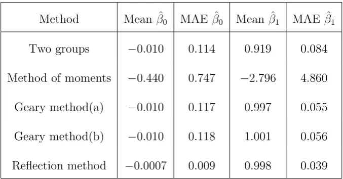
subject to measurement error (ME). The reflection method (RM) uses all observed data points, and does not exclude or ignore part of the data or replace them by ranks. The RM is straightforward, and easy to implement.
We show that the RM is equivalent or asymptotically equivalent to the or-thogonal regression method. Simulation studies show that the RM produces estimators that are nearly asymptotically unbiased and efficient under the
assumption that the ratio of the error variances λ = σ2ϵσδ−2 = 1. Moreover, it allows us to define the sum of squares error uniquely, the same way as in the case of no measurement error. The numerical comparisons of the results
1.3 Outline of the Thesis 15
Chapter 6 introduces a new slope estimator for regression model when both
variables are subject to measurement errors and the model includes equation error. The main aim of the proposed method is to improve the efficiency of Wald’s estimator under flexible assumption on the ratio of error variances (λ). It is well known that in the presence of equation error in regression models any estimator based on assumed knowledge of (λ) is biased. Although Wald’s method could deal with models that include equation error, it lacks efficiency
and is subject to identifiability problem. To compare the relative efficiency of the proposed estimator with the OLS, Wald’s and Geary’s estimators, simulation studies under various assumptions are undertaken. Moreover, a
comparison of the new estimator with the method of moments estimator when λ is biased due to the presence of the equation error is included. Chapter 7 introduces a new estimator to fit the regression line when both variables are subject to measurement errors and there is no prior information
known about the variances of error. The proposed weighted reduced major axis (WG) is derived based on the mathematical relationship between the vertical and orthogonal distances of the observed points and the regression
line. The geometric mean (GM) regression method is widely used in many disciplines as a solution to errors in variables model, although it lacks effi-ciency. To evaluate the geometric mean GM estimator method, this Chapter
not quite true, is that this method minimizes the vertical and horizontal
dis-tances between observed points and the best-fit straight line. We compare the performance of the proposed WG estimator with the GM and OLS-bisector estimators, and the sensitivity to the variation of the ratio of error variances
Chapter 2
Historical background of
measurement error models
2.1
Introduction
Currently, there is a huge literature on measurement error (ME) models
(Fuller, 2006; Carroll et al. 2006; Cheng and Van Ness, 1999; Gillard, 2010). The literature of ME has become widespread in diverse fields such as eco-nomics, medical science, agriculture, chemistry, physics, astronomy and
some of the common estimation techniques to deal with measurement
er-ror models, and discusses some interconnections between these methods. In fact, it is difficult to discuss the whole wealth of literature on measurement error models in this thesis, but the focus has been placed upon a few key
developments and methods. Unfortunately the notation set of the measure-ment error models has not been standardised in the literature, so it will be carefully introduced at the beginning of the thesis. The measurement error
problem is also known as error-in-variables or model II regression (cf Sokal and Rohlf, 1995, p. 541).
2.2
Major Axis Regression (Orthogonal)
The problem of fitting a simple linear regression model when both variables
are subject to error was first considered by Adcock (1877), where he intro-duced the major axis regression (MAR) technique which is also known as orthogonal regression (OR). However, this method is equivalent to the
bi-variate case of principal components analysis (PCA) (Mohler et al. 1978). Geometrical exposition of this method is to minimise the squared perpendicu-lar distances from the data points to the fitted regression line. The estimator
2.2 Major Axis Regression (Orthogonal) 19
technique is given by
ˆ
β1OR=
(S2
y −Sx2) +
√
(S2
y −Sx2)2+ 4Syx2
2Syx
,
whereS2
y is the sample variance of the manifest response variabley,Sx2 is the
sample variance of the manifest explanatory variablexandSyx is the sample
covariance of y and x.
An alternative form of this estimator is
ˆ
β1M A = 0.5 [
( ˆβ2−βˆ1−1) +sgn{Syx} √
4 + ( ˆβ2−βˆ1−1)2
]
,
where ˆβ1 =
Syx
S2
x
,and ˆβ2 =
S2
y
Syx
.
Adcock dealt with a special case of the problem of estimating β1 in the standard simple linear regression model, where there is no equation error.
This case assumes that the variances of measurement error in both variables are equal, that is, σ2
ϵ =σδ2, whereϵj is the measurement error in the manifest
response variable yj, (yj =ηj +ϵj), and δj is the measurement error in the
manifest explanatory variable xj, (xj =ξj +δj). Adcock defined the line of
the best fit through the data as the line which minimises the sum of squares of the orthogonal distances from the observed points to the fitted line. Whereas
the least squares method defines the line of the best fit which minimises the sum of squares vertical distances (residuals) as
n ∑
j=1
Adcock mentioned that the best regression line should pass through the mean
of the n points, wheren is the sample size.
Kummell (1879) extended the work of Adcock, where he assumed that the ratio of error variances λ = σ
2
ϵ
σ2
δ
was known instead of taking equal error variances,σ2
ϵ =σδ2. He justified this assumption since it is realistic that most
experienced practitioners will have sufficient knowledge about the spread of the measurement errors. Pearson (1901) suggested a very similar estimator to that proposed by Adcock (cf Fuller, 2006, p. 30). He showed that the
fitted regression line of this method always lies between the regression line of ξ on y and that of y on ξ. In addition, this technique does not depend on which variable is treated as response variable and which is explanatory
variable (cf Amman and Van Ness, 1988). Isobe et al. (1990) pointed out that the major axis regression is appropriate only for scale free variables, such as ratios of observable variables or logarithmical transformed variables.
2.3
Deming Regression Technique
2.3 Deming Regression Technique 21
the assumption that the ratio of error variances λ = σ 2
ϵ
σ2
δ
is known (Gillard, 2010). It takes measurement errors for both variables into account, therefore it is more generally applicable than major axis regression technique (Linnet,
1998). In his book, Deming (1943) suggested this technique to minimise the common error simultaneously to obtain the best line that fits the data. The
slope estimator of this technique is given by
ˆ
β1DEM =
(S2
y −λSx2) +
√
(S2
y −λSx2)2 + 4λSyx2
2Syx
.
Note that the slope estimator of Deming regression technique ˆβ1DEM becomes
the slope estimator of the orthogonal regression technique ˆβ1OR when σϵ2 =
σ2
δ, (λ= 1) (cf Gillard and Iles, 2009).
Fuller (2006, p. 30) stated the above estimator was first derived by Kummel
(1879) for a general λ, but he did not formulate the model in precisely the same manner. In clinical chemistry literature this technique is attributed to Deming (1943) (cf Linnet, 1998). It is also called orthogonal regression in
statistical literature. In his book, Fuller (2006, p. 30) called it a method of moments estimator (MOM), although it differs from the commonly used method of moments estimator (cf Carroll and Ruppert, 1996).
is aimed to minimise the error term. Deming regression solution is the major
axis regression solution when the ratio of error variances is equal to one, λ= 1. The major axis regression method is a special case of Deming regression method when the variance of error terms are equal σ2
ϵ =σ2δ.
The fundamental problem of using the Deming regression method arises when
the value of λ is not known with certainty (see Dunn, 2004). Carroll et al. (1995) and Carroll and Ruppert (1996) question if the assumption of the value ofλ is at all correct, and they concluded thatλis frequently incorrect. An inappropriateλ leads to biased estimates of parameterβ1 and this is why these critics claim that many if not all examples of Deming regression are flawed. The inclusion of the equation error in linear regression is a common
practice but this technique does not take it into account (see Carroll and Ruppert, 1996).
2.4
Grouping Method
Wald (1940) proposed an estimation method based on the grouping of the
data. It divides the observations on both response and explanatory variables into two groups, G1 and G2, where G1 contains the first half of the ordered observations and G2 contains the second half. The grouping is made based
2.4 Grouping Method 23
the line joining the group means provided consistent estimator for the slope
parameter of the simple linear regression model. Properties of this estimator can be found in Gupta and Amanullah (1970).
To explain the grouping method, suppose that the variablesξj andηj are
re-lated by the equationηj =β0+β1ξj with both variables are subject to random
measurement error. Let xj =ξj +δj and yj =ηj +ϵj, where xj and yj
rep-resent the manifest explanatory variable and the manifest response variable respectively. The measurement error in the manifest explanatory variable
xj is δj and in the manifest response variable yj is ϵj (Gillard, 2010). It is
well known, for both large and small sample cases, that the presence of mea-surement error in the explanatory variable makes the ordinary least squares
(OLS) estimator inconsistent and biased (see Barnett, 1969). Furthermore, it makes the maximum likelihood estimator unacceptable (see Kendall and Stuart, 1961, p. 383). In 1940 Wald pointed out that a consistent estimator
of β1 may be calculated if the following assumptions are met:
1. The random variablesϵ1, ϵ2, . . . , ϵnhave the same distribution and they
are uncorrelated, that is, E(ϵiϵj) = 0 for i̸=j, and the variance of ϵj,
σ2
ϵ =E(ϵiϵj), for i=j, is finite.
2. The random variablesδ1, δ2, . . . , δnhave the same distribution and they
σ2
δ =E(δiδj), fori=j, is finite.
3. The random variables ϵj and δj are uncorrelated, that is, E(ϵjδj) = 0,
for all j. 4.
∑n
j=k+1xj −
∑k
j=1xj
n >0 or ¯xk+1 >x¯k, where ¯xk+1 is the mean of the
group G2, ¯xkis the mean of the group G1,nis even (n= 2,4,6, . . . ,∞),
and k = n2. In other words, we can be sure that as n→ ∞,b1 does not approach zero (cf Madansky, 1959).
The observations are then divided into two groups based on the ranks of
the manifest explanatory variable xj, those above the median ofxj into one
group,G1 and those below the median into another group,G2. Then Wald’s estimator of β1 and β0 are given by
ˆ
β1W =
a1
b1
= (y1+. . .+yk)−(yk+1+. . .+yn) (x1+. . .+xk)−(xk+1+. . .+xn)
= y¯2−y¯1 ¯
x2−x¯1
,
where (¯x1,y¯1) are the means of (xj, yj) into groupG1, forj = 1,2,· · · , k, and
(¯x2,y¯2) are the means of (xj, yj) into group G2, for j =k+ 1, k+ 2,· · · , n.
Then ˆβ0W = ¯y−βˆ1x¯, where ¯y=
∑n
j=1yj
n , x¯=
∑n
j=1xj
n , and a1 =
(x1+. . .+xk)−(xk+1+. . .+xn)
n , and
b1 =
(y1+. . .+yk)−(yk+1+. . .+yn)
2.4 Grouping Method 25
The Wald’s technique was further developed by Bartlett (1949). It has been
suggested as a simple method to handle the problem of measurement error when both variables are subject to imprecision, and no knowledge of the error of measurement is available. Instead of dividing the ordered observations into
two groups, he proposed that greater efficiency would be obtained by dividing it into three groups, G1, G2 and G3. G1 and G3 are the outer groups, and G2 is the middle group.
Lindley (1947) proposed another grouping technique based on four groups.
It requires the calculation of two slope estimates, where the first estimator uses the first and third quarters as the two groups and the second estimator makes use of the second and fourth groups. The proposed estimator of this
technique is given by the mean of these two slope estimates.
Generally these grouping methods are designed to counter the problem of inconsistency. However, the groups are not independent of the error terms if they are not based on the order of the true values. But Wald proved that
the grouping by the observed values is the same as grouping with respect to the true values. There are some criticisms in the literature about Wald estimator but these lack consensus. Neyman and Scott (1951) pointed out
if and only if
P r[xp1 −ϵ < ξ ≤xp1 −µ] =P r[x1−p2 −ϵ < ξ < xp1−µ] = 0,
wherexp1 andx1−p2 are thep1and (1−p2) percentile points of the distribution function ofx, and ϵ−µis the range ofδ. This condition means that we must know the range of the error in x, and in order to satisfy the condition the range should be finite, otherwise the condition becomes P r[−∞< ξ <∞] = 0 which is never satisfied. Madansky (1959) pointed out that this condition
relies on the central limit theorem and assumes thatδis normally distributed. But this has an infinite range, and so the above condition remains unsatisfied when the errors δj are normally distributed (cf Madansky, 1959).
Wald’s estimator is consistent under very general conditions except where
the errors are not normally distributed (cf Gupta and Amanullah, 1970). Pakes (1982) claimed that the work of Gupta and Amanullah (1970) is need-less given that Wald’s estimator is inconsistent. However, according to Theil
(1956), Wald’s method is valuable though there is a loss of efficiency. John-ston (1972, p. 284) stated “Under fairly general conditions the Wald esti-mator is consistent but likely to have a large sampling variance”. Moreover,
Fuller (2006, p. 74) mentioned that the Wald’s method was often interpreted improperly.
group-2.5 Reduced Major Axis 27
ing method by dividing the observations to more than two groups and to
groups of unequal size (see Nair and Banerjee, 1942; Bartlett, 1949; Dorff and Gurland, 1961; Ware, 1972). In practice, the grouping method is still important and the grouping estimator is the maximum likelihood estimator
under the normality assumption (see Chang and Huang, 1997; Cheng and Van Ness, 1999, p. 130).
2.5
Reduced Major Axis
One of the simplest approaches to handle the error in variables is the
geomet-ric mean (GM) functional relationship, initially proposed by Teissier (1948) and later by Barker et al. (1988), and Draper and Yang (1997). This esti-mator has frequently been mentioned in the literature for two cases. First
is when there is no basis for distinguishing between the response and ex-planatory variables, and the second is to handle the errors-in-variables when the additional information is not available. The geometric mean functional
relationship is widely used in fisheries studies. It has received much atten-tion, and has been suggested that it is more useful than ordinary least squares (OLS) estimator for comparing the lean body proportions (Sprent and Dolby,
1980).
on xregression line, and the reciprocal of the slope of x ony regression line where x and y both are random (see Leng et al. 2007).
The GM estimator of the slope is given as
ˆ
β1G =sgn(SPxy) √
SSy
SSx
=sgn(Spxy) (
Sy
Sx )
,
where SSx = ∑n
j=1(xj−x¯)
2, SS
y =
∑n
j=1(yj−y¯)
2,
SPyx = ∑n
j=1(xj−x¯)(yj −y¯), and Sy and Sx are the standard deviation of
y and x respectively.
In the literature of biology and allometry the geometric mean method is known as the standardized major axis (MA) regression (Warton et al. 2006). It is also known as reduced major axis (RMA), or the line of organic
correla-tion (see Tessier, 1948; Kermack and Haldane, 1950; Ricker, 1973). Moreover, in physics it is known as a type of standard weighting model (see Machonald and Thompson, 1992), while the astronomers call it as Str¨omberg’s Impartial
Line (Feigelson and Babu, 1992).
A host of recent publications indicate that using the GM or RMA is necessary and sufficient to fit the straight line when the response and explanatory variables are both subject to error (cf Levinton and Allen, 2005; Zimmerman
2.5 Reduced Major Axis 29
is unbiased if and only if
λ= σ 2
ϵ
σ2
δ
= σ 2
y
σ2
x
.
But several studies indicate that this assumption is unrealistic (cf Sprent and Dolby, 1988).
There is a common recommendation to use GM estimator but is often em-ployed without mentioning the reason of using it (cf Smith, 2009). Jolicoeur
(1975) stated that is difficult to interpret the meaning of the slope estimated by the geometric mean method. However, the common perception is that the geometric mean method seeks to minimise the vertical and horizontal
dis-tances between the observed points and the fitted line (Halfon, 1985; Draper and Yang, 1997). But this is not quite true, given that the GM minimises the orthogonal distance of the observed points (xj, yj) from the unfitted line
2.6
Moments estimators
2.6.1
Estimators based on the first and second
mo-ments
The main problem in fitting the measurement error model using the method of moments is that of identifiability. Therefore, this method is based on the
assumption that some prior knowledge about the error variances is avail-able. Under this assumption the method of moments equations can easily be solved. Otherwise, it can be seen from equations (2.1-2.6) below that
a unique solution cannot be found for the parameters since there are five equations with six unknown parameters (Gillard, 2010). The expressions for population moments are
E[x] = E[ξ] =µ, and
E[y] = E[η] =β0+β1ξ.
The variances and covariance of the manifest variables are
var(x) = σξ2+σδ2,
var(y) = β12σξ2+σϵ2, and
2.6 Moments estimators 31
The estimating equations of the method of moments are found by equating
the above population moments to their sample equivalents as follows
¯
x = µˆx =
1
n
n ∑
j=1
xj, (2.1)
¯
y = βˆ0+ ˆβ1µˆx, (2.2)
Sx2 = ˆσ2ξ+ ˆσδ2, (2.3)
Sy2 = βˆ12σˆ2ξ + ˆσϵ2, (2.4)
Syx = βˆ1σˆ2ξ. (2.5)
Van Montfort (1989) introduced the hyperbolic relationship between the method of moments estimator for σ2
ϵ and σδ2 which is called the Frisch
hy-perbola, given as
(Sx2−σˆ2δ)(Sy2−σˆϵ2) = (Syx)2. (2.6)
This equation relates pairs of estimates (ˆσδ2,σˆ2ϵ), and it is also a useful equa-tion to derive another pairs of parameters such as
Sy2 = ˆβ1Syx+ ˆσ2ϵ.
However, to use the first and second moment estimating equations we should specify which assumptions of the parameter space is likely to suit the purpose in order to avoid the identifiability problem. Kendall and Stuart (1973),
The first assumption is that the intercept β0 is known. An estimator for the slope parameter β1 can be derived by using equations (2.1) and (2.2), and the estimator of the slope β1 is
ˆ
β1 = ¯
y−β0 ¯
x .
Dunn (2004) considered this assumption whenβ0 = 0, and he noted that this assumption is extremely unsafe. It is clear that the problem occurs with this estimator when ¯x ≈ 0. Therefore there are specific admissibility conditions for the estimator based on assumption that the intercept β0 is known which are
¯
x̸= 0,
Sx2 > σξ2, Sy2 > y¯−β0
¯
x Syx.
In fact, the assumption that the intercept β0 is known does not make the normal model of more than one explanatory variable identifiable (cf Cheng
and Van Ness, 1999, p. 6).
The second assumption is that the ratio of error variances λ = σϵ2σδ−2
is known, and that σ2
ξ > 0. Then equations (2.3), (2.4) and (2.5) yield the
following quadratic equation in ˆβ1 ˆ
2.6 Moments estimators 33
The positive root of this equation is the maximum likelihood solution which
can be expressed as
ˆ
β1 = (S2
y −λSx2) +
√
(S2
y −λSx2)2+ 4λSyx2
2Syx
. (2.7)
There are some equivalent forms of (2.7) such as
ˆ
β1 =
2λSyx
(S2
y −λSx2) +
√
(S2
y −λSx2)2+ 4λSyx2
,
and
ˆ
β1 = φ(λ) +sgn{Syx}(φ2(λ) +λ)
1 2, where φ(λ) = S2y−λSx2
2Syx .
Note all these forms are equivalent, and this solution is the same as that in Deming regression (cf Cheng and Van Ness, 1999, p. 17).
Riggs et al. (1978) recommended the use of this solution based on their
results of simulation studies, but they emphasized the importance of having a reliable prior knowledge of the ratio of error variances, λ. Edland (1996) pointed out that slope estimator of linear measurement error models based
on assumed knowledge of the ratio of error variances is biased if the under-lying linear relationship is anything other than a completely deterministic, law-like relationship. Lakshminarayanan and Gunst (1984) discussed the
The third assumption is the reliability ratioκ=σ2
ξσ−x2 is known. Then it
is possible to obtain an unbiased estimator of the slope parameterβ1. In fact, for some specific disciplines information about reliability ratio κis available, particularly in psychology, and sociology literature. For example, studies of
community loyalty, social consciousness, willingness to adopt new practices, managerial ability (cf Fuller, 2006, p. 5).
The slope estimator of y onx is biased when there is measurement error in
x, and the magnitude of this bias is the reliability ratio κ. The estimator based on the assumption that the reliability ratio is known is considered as a correction of the bias of the slope estimator for yonxregression. It is well known that
plimβˆ1x = β1+
Cov(xj, vj)
V ar(xj)
= β1−
β1σδ2
σ2
ξ +σ2δ
= β1
σ2
ξ
σ2
ξ +σ
2
δ
=β1
σ2
ξ
σ2
x
=β1κ.
Then if the reliability ratio κ is known, the unbiased estimator becomes ˆ
β1 = βˆ1xκ−1.
This estimator could be obtained from the first and second moment equa-tions by dividing equation (2.5) by equation (2.3) (cf Gillard, 2010). A more
2.6 Moments estimators 35
correction for attenuation.
The fourth assumption is that the error variance σ2
ϵ is known. Equation
(2.4) and (2.5) immediately give
ˆ
β1 = (S2
y −σϵ2)
Syx
.
The estimator based on the known error variance is a modification of the
reciprocal of the slope of the x on y regression. This modification is to sub-tract the known error varianceσ2
ϵ fromSy2 in the numerator of the estimator
(cf Cheng and Van Ness, 1999, p. 18).
The fifth assumption is that the error variance σ2
δ is known. Equations
(2.3) and (2.5) are used to obtain an estimator for the slope parameter β1. The equation (2.3) can be written in terms of σ2
ξ, if the error variance σδ2 is
known, as follows
ˆ
β1 =
Syx
S2
x−σδ2
.
max-imum likelihood estimator. These five restrictions are
Sx2 ≥ Syx
ˆ
β1
, (2.8)
Sy2 ≥ βˆ1Syx, (2.9)
Sx2 ≥ σˆδ2, (2.10)
Sy2 ≥ σˆϵ2, (2.11)
sgn(Syx) = sgn( ˆβ1). (2.12) If any one or all these conditions are not satisfied then the maximum likeli-hood solution is
ˆ
β1 =
S2
y
Syx
.
This estimator is just the reciprocal of the slope estimator of the inverse
regression of y onx ( Cheng and Ness, 1999, p. 18).
The sixth assumption is that both variances σδ2 and σϵ2 are known. In this case, any four of the moment equations (2.1) to (2.5) can be used to derive unique estimator. Based on this assumption the possible solutions of
estimating equations (2.1) to (2.5) are
1. If both error variancesσ2
δ, andσϵ2 are known, then the ratio of the error
variances is also known. This yields
ˆ
β1 =
(Sy2−λSx2) +
√
(S2
y −λSx2)2+ 4λSyx2
2Syx
2.6 Moments estimators 37
2. Substituting (2.4) into equation (2.5) yields the same estimator as when
σϵ2 is known
ˆ
β1 = (S2
y −σϵ2)
Syx
.
3. Another estimator for the slope parameterβ1is obtained by rearranging equation (2.4) in terms of β2
1σ2ξ and dividing by equation (2.3) which
yields
ˆ
β1 = sgn{Syx} √
S2
y −σϵ2
S2
x−σx2
.
4. Substituting (2.3) into equation (2.5) yields the same estimator as when
σδ2 is known:
ˆ
β1 =
Syx
S2
x−σδ2
.
All of the estimators outlined above are obtained by restricting the parameter space. If a restriction is unsatisfied, then the method of moment equations
are not useful. This is a problem due to having six unknown parameters, but only five moment estimating equations. However, the conditions basically suggests that the fitted regression line lies between the OLS line of y on x
2.6.2
The method of higher-order moments
One of the most widely known techniques for slope estimator of the simple linear regression model with measurement error is the method of higher-order
moments. Many statistical books have referred to this method and describe that the method of higher-order moments corresponding sample moments to parameter estimates such as Casella and Berger (1990). The method of
higher-order moments has a long history, yet it is still an effective tool, be-cause it is easily implemented (see Bowman and Shenton, 1988). Commonly, many statistical texts give greater attention to the method of higher-order
moments. The estimators of the method of higher-order moments are not uniquely defined and it is necessary to choose amongst possible estimates to find the best estimator to data. This may lead to the cases where the method
is used in measurement error models.
The first person to recognize the potential of population moments as a basis of estimation is Karl Pearson (1890). He introduced the method of moments (MM) estimation in a series of his papers published after 1890s. This method
has two fundamental features:
2.6 Moments estimators 39
2. It does not need to specify any sort of distribution and does not use any
information about the population distribution other than its moments.
Indeed, using the method of moments to handle the measurement error
prob-lem requires that some information regarding a parameter must be assumed to be known, or more estimating equations have to be derived by the higher moments (Cheng and Van Ness, 1999). Scott (1950) introduced an estimator
based on the third moments for the structural model, and showed that if the third central moment of ξ exists and is non-zero, then the equation is given by
fn,1( ˆβ1ξ) = ∑n
j=1[(yj−y¯)−βˆ1ξ(ξj−ξ¯)]3
n = 0,
where, he mentioned that, ˆβ1ξ is a consistent estimator ofβ1. This is because lim
n→∞fn,1( ˆβ1ξ) = (β1−
ˆ
β1ξ)3µ3ξ,
where µ3
ξ denotes the third central moment of ξ. He showed that the
esti-mator of the slope is a function of the third order sample moments. Scott
(1950) mentioned that estimators based on the lower order moments may be more accurate than those based on higher order moments. He introduced the estimator without a method of extracting the root which would provide
the consistent estimator (Gillard, 2010).
discussed some large sample properties. Drion (1951) mentioned that an
es-timator could be derived through the third-order non-central moment equa-tions for a functional model. Moreover, he introduced the variances of all the sample moments, and showed that his estimator of the slope is consistent,
and the sample moments are given by
Mrs(x, y) = ∑n
j=1(xj −x¯)r(yj −y¯)s
n , and Mrs′ (x, y) =
∑n
j=1x
r jysj
n ,
where rand s are order of moments, and ¯x= n1 ∑nj=1xj,and ¯y= 1n ∑n
j=1yj.
Pal (1980) and Van Montfort et al. (1987) introduced a treatment for the
structural relationship model under the assumption that the latent variable
ξ is not normally distributed and the moments exist. It is also assumed that the latent variableξj, the measurement error in the response variableϵj, and
the measurement error in the explanatory variable δj are independent of one
another. The equation error (q) is allowed in this approach by absorbing the e