A Bayesian High-Frequency Estimator of the Multivariate Covariance of Noisy and Asynchronous Returns

(1)

City, University of London Institutional Repository

Citation:

Peluso, S., Corsi, F. & Mira, A. (2015). A Bayesian High-Frequency Estimator of the Multivariate Covariance of Noisy and Asynchronous Returns. Journal of Financial Econometrics, 13(3), pp. 665-697. doi: 10.1093/jjfinec/nbu017

This is the draft version of the paper.

This version of the publication may differ from the final published

version.

Permanent repository link:

http://openaccess.city.ac.uk/19453/

Link to published version:

http://dx.doi.org/10.1093/jjfinec/nbu017

Copyright and reuse: City Research Online aims to make research

outputs of City, University of London available to a wider audience.

Copyright and Moral Rights remain with the author(s) and/or copyright

holders. URLs from City Research Online may be freely distributed and

linked to.

(2)

A Bayesian High-Frequency Estimator of the

Multivariate Covariance of Noisy and Asynchronous

Returns

Stefano Peluso, Fulvio Corsi and Antonietta Mira

Swiss Finance Institute, University of Lugano, Switzerland

January 2012

Abstract

A multivariate positive definite estimator of the covariance matrix of noisy and asynchronously observed asset returns is proposed. We adopt a Bayesian Dynamic Linear Model which allows us to interprete microstructure noise as measurement er-rors, and the asynchronous trading as missing observations in an otherwise synchronous series. These missing observations are treated as any other parameter of the problem as typically done in a Bayesian framework. We use an augmented Gibbs algorithm and thus sample the covariance matrix, the observational error variance matrix, the latent process and the missing observations of the noisy process from their full conditional distributions. Convergence issues and robustness of the Gibbs sampler are discussed. A simulation study compares our Bayesian estimator with recently proposed pair-wise QMLE-type and Multivariate Realized Kernel estimators, under different liquidity and microstructure noise conditions. The results suggest that our estimator is superior in terms of RMSE in both a two- and ten-dimensional settings, especially with dispersed and high missing percentages and with high noise. This suggests that our Bayesian estimator is more robust in severe conditions, such as portfolios of assets with het-erogeneous liquidity profiles, or particularly illiquid, or when there is a high level of microstructure noise in the market.

Keywords: Asinchronicity; Data Augmentation; Gibbs Sampler; Missing Observations;

Realized Covariance.

(3)

1 Introduction

Available intra-day prices can be used to improve the estimation of the covariance among

several financial assets, so that even the covariation of asset prices within the day can be

included in the inferential process. The two main concerns when dealing with several time

series of Ultra-High Frequency (UHF) prices is that they are observed at different trading

times and with microstructure noise. The first problem is known as asynchronicity of UHF

asset prices and its effect on the estimation of the covariance was first identified by Epps

(1979), who found that the correlation is biased toward zero as the sampling frequency

in-creases. The Realized Covariance estimator proposed by Hayashi and Yoshida (2005) (HY)

is unaffected by this asynchronicity problem. The second feature of UHF asset prices (and

in general of asset prices) is that they present a component due to the microstructure noise1_.

A consistent QMLE-type estimator of the high-frequency covariance of two assets observed

asynchronously with microstructure noise was introduced by Ait-Sahalia et al. (2010), and

this will be our first benchmark.

When instead of the covariance between two assets we consider the covariance matrix of

several assets, all estimators mentioned above, that successfully deal with the asynchronicity

and noise in the bivariate case, do not guarantee a positive semi-definite estimator in the

multivariate setting. To our knowledge, the only work in the literature proposing a

mul-tivariate covariance estimator that preserves positivity is the Mulmul-tivariate Realized Kernel

(MRK) of Barndorff-Nielsen et al. (2011), and this will provide our second benchmark. They

suggest to synchronize the high frequency prices using a Refresh Time Scheme combined with

a multivariate realized kernel to provide a consistent and positive semi-definite estimator of

1_{In the literature, there are several proposed corrections to HY that make it robust to this noise. For}

example, Voev and Lunde (2007), Bibinger (2011), based on a multiscale subsampling correction of HY that improves the convergence properties of the estimator proposed by Palandri (2006) and the Two-Scales Realized Covariance (TSRC) estimator of Zhang (2011).

(4)

the covariance matrix. A drawback of their methodology is that the synchronization of the

time series with the Refresh Time Scheme can cause a large loss of information if the involved

assets are traded with very different liquidity. Furthermore, they need to tune a bandwidth

parameter. Finally, their results are valid only asymptotically, when the mesh of trading

interval converges to zero and the number of observations goes to infinity: their simulation

study (limited to the bivariate case) shows that there is still an important bias due to the

finiteness of the sample and coarse trading intervals.

We are motivated by the need of an unbiased, positive-semidefinite estimator of the

multi-variate covariance matrix of asynchronous and noisy UHF asset prices. We cast the problem

into a Bayesian framework and consider the asynchronous times series as synchronous series

with missing observations, that are treated as any other parameter of the problem as

typi-cally done in a Bayesian framework. The flexibility of the dynamic linear model we adopt

allows us to easily treat the true latent price process, not affected by microstructure noise, as

additional parameters to be estimated. Since the joint posterior distribution of the

param-eters and the missing values is not standard, we use Markov chain Monte Carlo algorithms

to obtain samples from it. In particular, the posterior covariance matrix is sampled through

a Gibbs sampler from an Inverse Wishart distribution which naturally preserves its positivity.

We present our methodology in Section 2: in 2.1 we introduce the case of asynchronicity

without noise, which is extended in 2.2 to noisy observations and propose the augmented

Gibbs sampler. In Section 3 several Monte Carlo simulation experiments are performed to

compare our Bayesian estimators with the AFX estimator of Ait-Sahalia et al. (2010) and

the MRK estimator of Barndorff-Nielsen et al. (2011) in a bivariate (3.1) and multivariate

(3.2) setting. The results favour our estimator, particularly for a high number of assets and

(5)

its robustness to strong microstructure noise and high missings percentages in Sections 4.1

and 4.2, respectively. Section 5 concludes.

2 Methodology

2.1 Asynchronicity without noise

We start by considering the model with asynchronous prices that are observed at

differ-ent times within the day, but without being contaminated by microstructure noise. The

simplified model is

dXt =µ(Xt, θ)dt+

p

Σ(Xt, θ)dWt (1)

where, for some compact Θ ⊆ _Rk_, _θ _{the unknown parameter vector,} _µ _:

Rd ×Θ → Rd,

Σ :_Rd_×_Θ_→

Rd×d,+,Xtis ad-dimensional log-price diffusion process,Wtis ad-dimensional

Brownian motion and _Rd×d,+ _:= _{_M _∈

Rd×d : M > 0, symmetric}, that is the space

of square, d×d positive definite symmetric matrices. We assume that the drift and the

diffusion functions satisfy the Lipschitz condition

||µ(x, θ)−µ(y, θ)||+||pΣ(x, θ)−pΣ(y, θ)|| ≤C||x−y|| (2)

for some positive constant C and with || · || indicating the Euclidean norm. We need this

assumption to ensure the existence of a strong (unique), square integrable solutionXt to (1)

(Oksendal (2002)).

We work with the discretized version (∆t = 1) of (1) with constant diffusion coefficient

(6)

we recognize that the volatility is a time-varying process, but we are interested in the

estima-tion of a constant volatility parameter for each day. For this purpose we rely on the recent

result of Xiu (2010) that shows that the QMLE of the volatility of a misspecified model with

constant volatility remains consistent and optimal in terms of its rate of convergence under

fairly general assumptions. Let us first consider the bivariate case, for i= 1,2

Xi,t = Xi,t−1+i,t i,t ∼N(0, σi2), (3)

with corr(1,t2,t) = ρ, Xi,t is the log-price of asset i observed at time t, σi is its volatility

and ρ is the correlation coefficient.

We define Σ = 

 

σ2₁ ρσ1σ2

ρσ1σ2 σ22





, the missing and observed parts of X respectively as

Xmiss and Xobs and partition the time interval [1,· · · , T] as [tmiss

i ,tobsi ] accordingly. The

likelihood is

L(Σ,Xmiss_1:_T |Xobs_1:_T)∝

2

Y

i=1

1 (1−ρ2₎_σ2

i

exp



−

1 2

X

t∈tobs i

(Xi,t−mi,t)2 (1−ρ2₎_σ2

i



,

whereXi,s:t indicates the log price of asseti, from time sto time t, both extremes included,

mi,t := Xi,t−1−ρ_σσ₋i

i(X−i,t−X−i,t−1) and −i is the other asset. We assume a Jeffrey’s

un-informative prior for Σ, p(Σ) ∼ |Σ|−3/2_{, but an informative prior that incorporates in the}

analysis prior knowledge on the problem can easily be adopted. For example, in an

empir-ical Bayesian approach, an Inverse Wishart prior for Σ, with parameters T0 and S0 being

respectively, the sample size and the sum of squared observed returns, ignoring the missing

data, would still retain the conjugacy of the problem.

The asynchronicity (or, in other words, the presence of missing observations) complicates

(7)

standard results from multivariate normal theory to derive the full conditional for Σ:

p(Σ|X)∝ |Σ|−(T+3)/2exp −1

2tr(Σ

−1

T

X

t=1

t0t)

!

∝IW T

X

t=1

(Xt−Xt−1)(Xt−Xt−1)0, T

!

and find that φ(Xmiss

i,t |Σ), the full conditionals ofXi,tmiss, i= 1,2, are normal:

X_i,tmiss|X_i,_1:_t−1, X−i,1:t,Σ∼N mi,t,(1−ρ2)σi2

,

where the subscript −i refer to the other asset. The extension of (3) to the multivariate

case is straightforward and sampling the covariance matrix from an Inverse Wishart assures

that the resulting estimate is positive definite. As mentioned in the introduction, up to our

knowledge, this is the first attempt to have a positive definite multivariate estimator, besides

?, who operate in a frequentist context and pay the price of disregarding many observations,

due to the Refresh Time Scheme they adopt. The generic d-dimensional discretized model

is, fori= 1,· · · , d:

Xi,t = Xi,t−1+i,t i,t ∼N(0, σi2), (4)

with corr(i,tj,t) =ρij. X and Σ are, respectively, ad x T and adx d matrix. We write the

likelihood as

L(Σ,Xmiss_1:_T |Xobs_1:_T)∝ d

Y

i=1

v_i−1exp



−

1 2

X

t∈tobs i

v−_i 1(Xi,t−mi,t˜ )2



,

where vi := σi2 − Σ12Σ−221Σ

0

12, Σ22 is obtained from Σ by dropping the row and column

corresponding to asset i, whilst Σ12 is the i-th row of Σ without its i-th element, ˜mi,t :=

Xi,t−1+ Σ12Σ22−1(X−i,t−X−i,t−1) and X−i,s:t is the matrix of assets log prices j, ∀j 6=i and

from timesto timet. We have suppressed the dependence of Σ12 and Σ22 onifor notational

(8)

conditional is

p(Σ|X)∝ |Σ|−(T+d+1)/2exp −1

2tr(Σ

−1

T

X

t=1

t0t)

!

∝IW T

X

t=1

(Xt−Xt−1)(Xt−Xt−1)0, T

!

The full conditional of X_i,tmiss,φ(X_i,tmiss|Σ), is easily derived as:

X_i,tmiss|Xi,1:t−1,X−i,1:t,Σ∼N( ˜mi,t, vi).

To sample from the posterior distribution of Xmiss _{and Σ, we use a Gibbs sampler and}

iteratively sample {Xmiss,Σ} from their full conditionals. The algorithm at each iteration

thus consists of the following two steps:

1. Draw a covariance matrix Σ from its full conditional, that is an Inverse Wishart

dis-tribution, IW(S(Xmiss), T), with S(Xmiss) = PT

t=1(Xt −Xt−1)(Xt −Xt−1)0. S is

expressed as a function of Xmiss to highlight the dependence on the imputed missing

log prices.

2. Impute the missing observations, Xmiss, by drawing from φ(Xmiss

i,t |Σ), ∀t ∈ tmiss, i =

1,· · ·, d.

2.2 Asynchronicity and noise

A step toward a more realistic model is made by introducing the microstructure noise, so

that our model becomes, for t= 1,· · · , T

Yt = Xt+ √

ΩdBt (5)

dXt = µ(Xt, θ)dt+

p

Σ(Xt, θ)dWt, (6)

whereµ, Σ, XtandWtare defined as in (1), Ω is the constant variance of the microstructure

(9)

-dimensional Brownian motion,Bt⊥Wt. Assume that the Lipschitz condition (2) is satisfied.

The discretized version of (5) and (6) with constant diffusion coefficient is

Yt = Xt+ηt , ηt∼N(0,Ω), (7)

Xt = Xt−1+t , t∼N(0,Σ), (8)

where Yt is the observed log-price, Xt is considered as the true latent log-price process,

ηt is the microstructure noise and Ω its covariance matrix, is the true latent return with

covariance Σ. ηt and t are assumed independent.

This is a linear state space model, consisting in the observation equation (7) and the state

equation (8). In this particular form, is also known in the literature as local level model, or

random walk plus noise model or steady forecasting model, extensively covered in Harvey

(1989) and in West and Harrison (1997). Despite its simplicity, the local level model can be

used to analyse real data sets in various settings and scenarios, as it has been pointed out by

many authors, see e.g. Durbin (2004) or Triantafyllopoulos (2010). The model can also be

viewed as a particular case of a Dynamic Linear Model (West and Harrison (1997)), DLM in

short, characterized in its general form by{A, C, R, Q}, respectively the observation matrix,

transition matrix, observation error variance matrix and transition error variance matrix,

possibly time-varying. Then, our model is a time-invariant DLM with matrices{Id, Id,Ω,Σ}.

Under this model, the observed log-return follows an MA(1) process (Ait-Sahalia et al.

(2010)), and we can still obtain the likelihood in a product form by noting that{t|Yt,Xt−1,Ω}Tt=1

are i.n.i.d (independent but not identically distributed) Gaussian random vectors with zero

means and covariance matrix ˜Σt = Vtt−1 + Ω. V

t−1

(10)

obtained through the Kalman filter. Hence, the likelihood is

L(Σ,Ω,Ymiss_1:_T ,X1:T|Yobs1:T)∝ d

Y

i=1

Y

t∈tobs i

˜

v_i,t−1exp

−1

2˜v

−1

i,t (Xi,t−m˜i,t)2

,

with ˜vi,t := ˜σ2i,t−Σ˜12,tΣ˜−221,tΣ˜012,t and Y miss

andYobs are the missing and observed parts of Y

corresponding to the partition [tmiss,tobs]. If we assume uninformative Jeffrey’s priors for Σ

and Ω, the complete date joint posterior density of Σ and Ω is proportional to

(|Ω||Σ|)−d+12

T

Y

t=1

N(Yt;Xt,Ω)N(Xt;Xt−1,Σ).

The Gibbs sampler can be used also in this more complicated setting since the full

con-ditionals are available in standard form. In our simulation approach, we augment the data

twice, by considering both the missing observations and the latent process as additional

pa-rameters. Therefore, we implement the algorithm by iteratively sampling {X,Σ,Ω,Ymiss}

from their full conditional densities. The full conditionals of Σ and Ω are still proportional

to Inverse Wishart: p(Σ|Ω,Y1:t,X1:t)∝IW(SSΣ, T)and p(Ω|Σ,Y1:t,X1:t)∝IW(SSΩ, T), with

SSΣ=

PT

t=1(Xt−Xt−1)(Xt−Xt−1)

0_and _SS

Ω =

PT

t=1(Yt−Xt)(Yt−Xt)

0_.

To sample the missing observations, we partition Y in [Ymiss,Yobs] and the full

condi-tional density of the missing observations are still available in a standard form since they

are obtained as the conditional normal density that result from the joint density of observed

and missing log-prices Yt|Y1:t−1,X,Σ,Ω ∝N(Xt,Ω), that is Yi,tmiss|Yi,1:t−1,Y−i,1:t,X,Σ,Ω,

distributed as N Xi,t+ Ω12Ω−221(Y−i,t−X−i,t), ωi2−Ω12Ω−221Ω012

, where Y−i,s:t is the matrix

of log-prices for assets j, ∀j 6=i, from time s to time t and, similarly, X−i,s:t is the matrix

of latent log-prices sampled with the FFBS algorithm for assets j, ∀j 6= i and from time s

to time t. Ω22 is obtained from Ω by dropping the row and column corresponding to asseti,

(11)

Finally, we extract the latent log-priceby using the FFBS (Forward Filtering Backward

Simulation) algorithm, a Kalman smoother in which the smoothing recursions are replaced

by simulations of the latent process. Following Fruwirth-Schnatter (1994), we can write the

distribution of X|Y,Σ,Ω as

p(X|Y,Σ,Ω) =

T

Y

t=1

p(Xt|Xt+1:T,Y) (9)

where the last factor in the product is simplyp(XT|Y), i.e., the filtering distribution of XT,

which is N(Xt_t, Vt

t), with X

t

t the filtered latent log-price and Vtt its covariance matrix. In

order to obtain a draw from the distribution on the left-hand side, one can start by

draw-ing XT from N(Xtt, Vtt) and then, for t = T −1, T −2,· · · ,1, recursively draw Xt from

p(Xt|Xt+1:T,Y). It can be shown that p(Xt|Xt+1:T,Y) = p(Xt|Xt+1,Y1:t) and this

distri-bution is N(Xt_t+V_tt(V_tt₊₁)−1(Xt+1 −Xtt+1), Vtt−Vtt(Vtt+1)−1Vtt), where X

t

t+1 is the predicted

latent log-price.

Summarizing, the implemented Gibbs sampler executes the following steps at each

iter-ation:

1. Draw the covariance matrix Σ from its full conditional, that is an Inverse Wishart

distribution IW(SSΣ, T), with SSΣ=PTt=1(Xt−Xt−1)(Xt−Xt−1)0.

2. Draw the covariance matrix Ω from its full conditional, that is an Inverse Wishart

distribution IW(SSΩ, T), with SSΩ=PTt=1(Yt−Xt)(Yt−Xt)0.

3. Impute, for i= 1,· · · , d andt∈tmiss

i , the missing observationsY

miss _{by drawing from}

N Xi,t+ Ω12Ω−221(Y−i,t−X−i,t), ωi2−Ω12Ω−221Ω012

,where the dependence oniof Ω12and

(12)

its full conditionalQT

t=1N(mt, Wt), where we have defined mt≡X

t

t+Vtt(Vtt+1)−1(Xt+1−

X_tt₊₁)and Wt≡Vtt−Vtt(Vtt+1)−1Vtt.

3 Simulation Study

In this section we compare the performance of our Gibbs estimator with other estimators

available in the literature. The first alternative is proposed by Ait-Sahalia et al. (2010)

(AFX), who estimate the covariance as a function of variances after sinchronizing the asset

returns. They use the Refresh Time Scheme introduced by?, which consists in aligning the

returns on an irregular time grid by selecting those ticks at which all the assets have been

traded at least once in the interval. This scheme includes the largest amount of data among

all the Generalized Synchronization Schemes as defined in Ait-Sahalia et al. (2010), but

the loss of information still strongly depends on the presence of illiquid assets since several

observations for the more liquid assets are neglected within each grid interval. After the

sinchronization, they estimate the covariance by applying the QMLE estimator suggested in

Ait-Sahalia et al. (2005) to the identity Cov(X1, X2) = 1₄(Var(X1+X2)−Var(X1−X2)), valid

for any random variables X1 and X2.

The second estimator we include in the comparison study is the Multivariate Realized

Kernel of Barndorff-Nielsen et al. (2011) (MRK). MRK synchronizes the high frequency

prices using a Refresh Time Scheme combined with a multivariate realized kernel to provide

a consistent and positive semi-definite estimator of the covariance matrix. In particular, for

its implementation, we choose a jittering parameter equal to 2 and a Parzen kernel

func-tion as weigth funcfunc-tion for the realized autocovariances. The bandwidth of each series is

computed using the true Σ and Ω and the multivariate bandwidth is chosen to be the

(13)

using the true Σ and Ω (that cannot be observed in reality) and thus we favour the MRK

methodology. For more details, we refer the reader to the original paper. To our knowledge,

this is the only estimator that guarantees that the estimated multivariate covariance matrix

is positive semidefinite. This property is essential in many applications and, to enforce it,

when using Ait-Sahalia et al. (2010) in a multivariate setting, it is suggested to project the

resulting estimated matrix into the space of positive semi-definite matrices, by minimizing

some notion of distance between the two matrices. The main problem with this projection

is that we can lose the financial interpretation of the covariance between the assets since, as

noted in Frigessi et al. (2010), some entries of the covariance matrix, upon projection, can

dramatically change.

We further report the results of the estimator proposed by Hayashi and Yoshida (2005)

(HY), that is the cross-product of all returns with at least a partial overlapping. HY is

robust to the asynchronicity but not to the microstructure noise. In our simulation study,

we pretend to observe the latent log-price process, in order to apply this estimator to the

latent log-prices free of noise, so that this becomes, in our setting, a benchmark unattainable

in real applications.

The data generating process is the stochastic volatility model of Heston (1993), for i=

1,· · · , dand t= 1,· · · , T:

dXi,t = σi,tdWi,t,

dσ_i,t2 = ki(¯σi2−σi,t2 ) +siσi,tdBi,t,

where E(dWi,tdWj,t) =ρijdt, E(dWi,tdBj,t) =δijπidt. We use an Euler discretization scheme

(14)

distribution Γ(2kiσ¯2i/si2, s2i/2ki) centered in the mean variance. All the codes have been

written in Matlab 7.11.0 (R2010b) and run (possibly in parallel) with Intel(R) Xeon(R)

CPU X7460 @ 2.66 GHz.

3.1 Bivariate case

To replicate the same setting adopted in Ait-Sahalia et al. (2010), we first run a bivariate

simulation study with: sample size of T = 10000, 1/3 and 1/2 of the observations removed

completely at random from the whole generated sample, for the first and second asset,

respectively, and two starting log prices of log(100) and log(40). The true mean covariance

matrix of the returns and the covariance matrix of the microstructure noise are, respectively,

Σ =



 

0.16 0.06 0.06 0.09





 , Ω =



 

0.08 0 0 0.04





.

The other parameters {ki, si, πi} of the Heston model are {6,0.5,−0.6} and {4,0.3,−0.75}

for asset 1 and 2 respectively. For comparison purposes, all parameter values are chosen as

in Ait-Sahalia et al. (2010). For each compared estimator we generate M = 100 matrices

of prices and we run our Gibbs sampler for each generated sample of prices for 5000 steps,

after 5000 initial iterations of burn-in. The starting point (of the MCMC simulation) of the

missing values is the local mean ignoring the missing data up to 10 ticks before and after

the missing trade. To speed up the convergence of the Markov chain, we need to be careful

about the initial values for the covariance parameters: We initialize the sampler from the

pairwise Hayashi and Yoshida (2005) estimate of the covariance of the partially observed

noisy returns series for the off-diagonal terms. As for the variances, we use the Two Time

Scale Estimator of Zhang et al. (2005). Then, we interpret the return variability not

cap-tured by the Two Time Scale Estimator as explained by the microstructure noise. We stress

(15)

not the validity of the results, since the chain is independent on the chosen starting values,

once it has reached stationarity. We report the results of this first simulation in Table 1,

together with the HY estimator proposed by Hayashi and Yoshida (2005), applied to the

latent log-prices free of noise, as unattainable benchmark.

On average, the Gibbs estimator performs better than all other methods in terms of

RMSE and bias. The MRK, the only direct competitor in the multivariate setting, has an

important bias and is more volatile. This could be quite relevant in empirical studies if we

also consider that the results for MRK are obtained with optimal bandwidth parameters

computed from the true unobserved Ω and Σ.

3.2 Multivariate case

For the multivariate simulation analysis, we estimate the covariance matrix for a portfolio

of 10 assets. Our Gibbs estimator is naturally extended to the 10-dimensional case, as the

MRK estimator. If the covariance matrix obtained with the pointwise AFX procedure is not

positive semi-definite, we project it onto the space of positive semi-definite matrices by

min-imizing the Frobenius distance. This projection is done following Higham (2002) algorithm,

slightly modified to avoid singular matrices. We also estimate with HY each off-diagonal term

of the covariance matrix for comparison purposes. The true data generating process variance

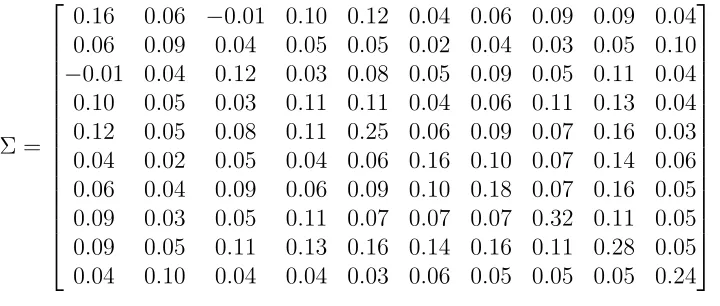
matrices are Σ, reported in Table 2, andΩ = diag([0.08,0.04,0.02,0.05,0.1,0.06,0.1,0.15,0.15,0.08]).

The simulation is initialized fromP0=log([100,40,60,80,40,20,90,30,50,60]), with

probabili-ties of missing observations for each series equal to{1/2,1/3,1/2,1/4,1/4,1/3,1/5,1/4,1/3,1/4}.

We note that, as the dimension of the portfolio increases, it becomes more and more difficult

to obtain ,through pairwise inferences, an estimated covariance matrix that retains

(16)

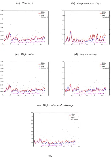
We iterate a random scan Gibbs sampler for 5000 (burn-in) plus 5000 steps and summarize

the results in Figure 1a that shows the RMSE of the estimators. We need to project the

pair-wise AFX onto the space of positive semidefinite matrices for 27 cases out of 100 Monte Carlo

simulations. The superiority of the Bayesian estimator relative to MRK is clear, since the

lat-ter is both more biased and volatile. As synthetic measure of the performance we choose the

Frobenius norm of the matrix difference ∆ between the estimated and the true (used to

gen-erate the data) covariance matrix. In particular, we define our norm as||∆i,j||=||( ˆΣji−Σ)||F,

where||·||F is the traditional Frobenius norm, and ˆΣji is thej-th covariance matrix estimated

with methodology i, with i ∈ {Gibbs, AF X, M RK} and j = 1, . . . , M. We further define

ˆ

E[||∆i||] := _M1

PM

j=1||∆i,j|| and ˆσ[||∆i||] :=

1

M−1

PM

j=1(||∆i,j|| −Eˆ[||∆i||])2

1/2

as the

es-timated expected value and standard deviation of the Frobenius distance for methodology

i. The relative values are reported in Table 3 and they suggest that the results favour our

multivariate Bayesian estimator, with MRK performing worst. In Figure 2a we compare

graphically the kernel density of the Frobenius distances for the three methodologies and

again we observe that the Gibbs estimator has the best performance, followed by AFX and

MRK.

We believe that the performance of the Bayesian estimator should improve relative to that

of AFX when we use more dispersed probabilities of observing missing values, that is assets

with very different liquidity, since in this case our naturally multivariate Bayesian estimator

catches information that the pairwise AFX cannot use. To validate this expected result, we

repeat the simulations for 10 assets, holding everything as in the previous simulation setting,

but with more dispersed missing probabilities {0,0.5,0.8,0.9,0.25,0,0.5,0.8,0.9,0.25}. The

results in Figure 1b confirm our intuition: now the pairwise nature of the AFX methodology

(17)

estimated by AFX 73% of the times. The relative norms are summarized in Table 3 and

in Figure 2b the relative kernel densities estimates are plotted. The explanation we give

is that information contained in the co-movement of more liquid assets is incorporated in

the estimation of covariances of less liquid asset only with a multivariate approach. The

improvement of the resulting estimates can be quite important in portfolios containing assets

with very different liquidity profiles.

4 MCMC convergence issues and robustness

Our model with noise is a non stationary latent Gaussian Bayesian model with Gaussian

response variables and we use an MCMC approach for inference. It is well known that

MCMC tends to exhibit poor performance when applied to these models. The first reason

is that the different points of the latent process X are strongly dependent on each other.

Second, the latent process and Σ are also strongly dependent, especially in large sample

settings as ours. This is known in the literature as Roberts-Stramer critique (Roberts and

Stramer (2001)) and is formalized by noting that

plim

∆t→0

T

X

t=1

(Xt−Xt−1)0(Xt−Xt−1) = Σ. (10)

This asymptotic relationship between Σ and X causes, in the limit, the Markov Chain

to be reducible, that is unable to escape from the current value.

A common approach to overcome the strong posterior dependencewithin the latent

pro-cess, is to sample the whole processX jointly. This is what we do in (9) by using the FFBS

algorithm of Fruwirth-Schnatter (1994) and the simulation study results suggest that our

(18)

ues of the noisy observed process adds a disturbance element to the sampling of the latent

process, breaking the deterministic relation between Σ andX. Our doubly augmented

algo-rithm naturally complements the traditional Gibbs sampler that does not sampleYmiss: the

convergence speed of the traditional Gibbs sampler increases when the signal-to-noise ratio

of the problem is higher (Roberts and Sahu (1997)), whilst in our augmented Gibbs sampler,

as the observational noise increases, sampling ofX will be more ”disturbed” by sampling of

Ymiss, improving the performance of the Bayesian estimator.

We investigate the robustness of our methodology in two ways: we increase the noise,

everything else being fixed, and look at simulation results to validate the hypothesis that

with higher noise, the Gibbs sampler works relatively better. Then, to test the robustness to

a finer grid, that is to a higher number of points between observations in the latent process,

we increase the missing percentage, holding everything else constant.

With an increase in noise, Ymiss introduces an higher ”disturbance” to the deterministic

relation (10) between the latent process and the covariance matrix. Since the reducibility

problem is attenuated, it is natural to expect that the Bayesian estimation improves relative

to the alternative methodologies. In Figure 1c we report the results for the different

method-ologies compared, with noise variance Ω1 = Ω + 0.35, and we indeed note that there is an

improvement in favor of the Bayesian approach. We project AFX 29% of the times to obtain

a positive definite covariance matrix. The estimated expected values and standard

devia-tions of the Frobenius distances are reported in Table 3, Figure 1c compares the RMSEs and

components of the methodologies and Figure 2c plots the Frobenius distance kernel densities.

The increase in missing percentage has the effect of increasing the number of points of

(19)

probabilities equal to the missing percentages of the standard multivariate case plus 0.35,

the simulation study shows superior results for the Bayesian estimator as reported in Figures

1d, 2d and in Table 3. AFX is projected 60% of the times to guarantee the positivity of

the estimated covariance matrix. We thus conclude that the other estimation procedures

deteriorate more rapidly than our as the conditions become more severe.

Finally, we add simultaneously more variance noise and more missings and we report the

results in Figures 1e, 2e and in Table 3, confirming the higher robustness of the Bayesian

methodology to more extreme market conditions. AFX has been projected 59% of the times.

For clarification, we stress the difference between the two Frobenius distances so far

mentioned in the text. The Frobenius used in the projection of AFX, is the distance between

the (non necessarily positive) covariance matrix estimated with AFX methodology and the

closest positive definite matrix. Its purpose is to minimize the impact of the projection. On

the other hand, the Frobenius shown in the Figures, is the distance between the covariance

matrix estimated by the generic methodology and the true covariance matrix. Its purpose is

to compare the performances of the estimators. It is reasonable to expect that the projection

negatively affects the performance of the AFX estimator, but results not reported (available

upon request) show that the impact of the projection is negligible.

5 Conclusions

In this paper we study the problem of estimation of the multivariate covariance matrix of

noisy and asynchronous observations. The Dynamic Linear Model is the setting chosen

to deal with presence of noise in the data, and we treat the asynchronous time series as

(20)

with missing observations (asynchronicity) by treating them as additional parameters of the

problem. An augmented Gibbs algorithm is implemented to sample the covariance matrix,

the observational error variance matrix, the latent process and the missing observations of the

noisy process. Our MCMC estimator is positive definite by construction and we compare

it with the bivariate estimator of Ait-Sahalia et al. (2010) (AFX) and the Multivariate

Realized Kernel (MRK) of Barndorff-Nielsen et al. (2011). A simulation study suggests

that our estimator is superior in terms of RMSE in a two- and ten-dimensional setting,

especially with dispersed and high missing percentages and with high noise. This suggests

that MRK and AFX perform worse than our Bayesian estimator in severe conditions, as

with portfolios of assets with heterogeneous liquidity profiles, or particularly illiquid, or

when there is a high level of microstructure noise in the market. We naturally overcome

the Roberts-Stramer reducibility critique (Roberts and Stramer (2001)) without losing the

conjugacy of the problem, by sampling the missing observations of the noisy process. As

possible extension, our methodology could be applied to factors of much larger portfolios.

Furthermore, we could extend the simulation algorithm to adaptive MCMC samplers (Haario

et al. (2001)) or to Particle MCMC methods (Andrieu et al. (2010)) to face the problem of

lost conjugacy of the full conditionals in case of non-linear and non-normal measurement

and transition equations.

References

Ait-Sahalia, Y., Fan, J., and Xiu, D. (2010). High-Frequency Covariance Estimates with Noisy and Asynchronous Financial Data.Journal of the American Statistical Association, 105:1504– 1517.

Ait-Sahalia, Y., Mykland, P., and Zhang, L. (2005). How Often to Sample a Continuous-Time Process in the presence of Market Microstructure Noise. The Review of Financial Studies, 18:351–416.

Andrieu, C., Doucet, A., and Holenstein, R. (2010). Particle Markov Chain Monte Carlo Meth-ods.Journal of Royal Statistical Society B, 72:269–342.

(21)

With Noise and Non-Synchronous Trading.Journal of Econometrics, 162:149–169.

Bibinger, M. (2011). Efficient Covariance Estimation for Asynchronous Noisy High-Frequency Data.Scandinavian Journal of Statistics, 38:23–45.

Durbin, P. (2004). Introduction to State Space Time Series Analysis. Cambridge: Cambridge University Press.

Epps, T. (1979). Comovements in Stock Prices in the Very Short Run.Journal of the American Statistical Association, 74:291–296.

Frigessi, A., Loland, A., Pievatolo, A., and Ruggeri, F. (2010). Statistical Rehabilitation of Improper Correlation Matrices. Quantitative Finance. iFirst.

Fruwirth-Schnatter, S. (1994). Data Augmentation and Dynamic Linear Models.Journal of Time Series Analysis, 15:183–202.

Haario, H., Saksman, E., and Tamminen, J. (2001). An Adaptive Metropolis Algorithm.

Bernoulli, 7:223–242.

Harvey, A. (1989).Forecasting Structural Time Series Model and the Kalman Filter. Cambridge: Cambridge University Press.

Hayashi, T. and Yoshida, N. (2005). On Covariance Estimation of Non-Synchronously Observed Diffusion Processes. Bernoulli, 11:359–379.

Heston, S. (1993). A Closed-Form Solution for Options with Stochatic Volatility with Applica-tions to Bond and Currency OpApplica-tions.The Review of Financial Studies, 6:327–343.

Higham, J. (2002). Computing the Nearest Correlation Matrix: a Problem from Finance. IMA Journal of Numerical Analysis, 22:329–343.

Oksendal, B. (2002).Stochastic Differential Equations. An Introduction with Applications. New York: Springer Verlag.

Palandri, A. (2006). Consistent Realized Covariance for Asynchronous Observations Contami-nated by Market Microstructure Noise. Technical report, University of Copenhagen.

Roberts, G. and Sahu, S. (1997). Updating Schemes, Correlation Structure, Blocking and Pa-rameterization for the Gibbs Sampler.Journal of Royal Statistical Society B, 59:291–317. Roberts, G. and Stramer, O. (2001). On Inference for Partially-Observed Nonlinear Diffusion

Models Using the Metropolis-Hastings Algorithm. Biometrika, 88:603–621.

Triantafyllopoulos, K. (2010). Real-Time Covariance Estimation for the Local Level Model. Jour-nal of Time Series AJour-nalysis.

Voev, V. and Lunde, A. (2007). Integrated Covariance Estimation using High Frequency Data in the Presence of Noise.Journal of Financial Econometrics, 5:68–104.

West, M. and Harrison, P. (1997). Bayesian Forecasting and Dynamic Models. New York: Springer Verlag.

Xiu, D. (2010). Quasi-Maximum Likelihood Estimation of Volatility With High Frequency Data.

Journal of Econometrics, 159:235–250.

(22)

(23)

[image:23.612.189.420.167.328.2]

6 Tables and Figures

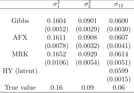
Table 1: Simulation results: bivariate case.M= 100 Monte Carlo estimates for each compared estimator are computed and

the mean is reported. The Gibbs sampler runs for 5000 iterations, plus 5000 of burn-in. The RMSE is reported in parenthesis. The HY estimator is the ideal benchmark computed on the unobserved latent process.

σ₁2 σ₂2 σ12

Gibbs 0.1604 0.0901 0.0600

(0.0052) (0.0029) (0.0030)

AFX 0.1611 0.0908 0.0607

(0.0078) (0.0032) (0.0041)

MRK 0.1652 0.0929 0.0614

(0.0106) (0.0054) (0.0051)

HY (latent) 0.0599

(0.0015)

(24)

[image:24.612.128.488.317.470.2]

Table 2: 10-dimensional state covariance matrix used to generate simulated data.

Σ = 

              

0.16 0.06 −0.01 0.10 0.12 0.04 0.06 0.09 0.09 0.04

0.06 0.09 0.04 0.05 0.05 0.02 0.04 0.03 0.05 0.10

−0.01 0.04 0.12 0.03 0.08 0.05 0.09 0.05 0.11 0.04

0.10 0.05 0.03 0.11 0.11 0.04 0.06 0.11 0.13 0.04

0.12 0.05 0.08 0.11 0.25 0.06 0.09 0.07 0.16 0.03

0.04 0.02 0.05 0.04 0.06 0.16 0.10 0.07 0.14 0.06

0.06 0.04 0.09 0.06 0.09 0.10 0.18 0.07 0.16 0.05

0.09 0.03 0.05 0.11 0.07 0.07 0.07 0.32 0.11 0.05

0.09 0.05 0.11 0.13 0.16 0.14 0.16 0.11 0.28 0.05

0.04 0.10 0.04 0.04 0.03 0.06 0.05 0.05 0.05 0.24



              

(25)

[image:25.612.159.449.311.560.2]

Table 3: Estimated expected values and standard deviations of the Frobenius distances between the estimated and the true covariance matrix. Eˆ[||∆i||] := M1

PM

j=1||∆i,j|| and ˆσ[||∆i||] :=

1

M−1

PM

j=1(||∆i,j|| −Eˆ[||∆i||])2

1/2

, with

M = 100 and 10 assets. Define missing probabilitiesv = {1/2,1/3,1/2,1/4,1/4,1/3,1/5,1/4,1/3,1/4} and noise matrix Ω = diag([0.08,0.04,0.02,0.05,0.1,0.06,0.1,0.15,0.15,0.08])

(a)Standard: missing probabilitiesvand noise matrix Ω.

(b)Dispersed missings: more dispersed missing probabilities{0,0.5,0.8,0.9,0.25,0,0.5,0.8,0.9,0.25}and noise matrix Ω. (c)High noise: missing probabilitiesvand noise matrix Ω + 0.35.

(d)High missings: missing probabilitiesv+ 0.35 and noise matrix Ω.

(e)High noise and missings: missing probabilitiesv+ 0.35 and noise matrix Ω + 0.35.

Gibbs AFX MRK

(a) Standard

ˆ

E[||∆i||] 0.0560 0.0622 0.1063

ˆ

σ[||∆i||] 0.0142 0.0137 0.0314

(b) Dispersed missings

ˆ

E[||∆i||] 0.0790 0.1164 0.1930

ˆ

σ[||∆i||] 0.0184 0.0259 0.0624

(c) High noise

ˆ

E[||∆i||] 0.0641 0.0759 0.1669

ˆ

σ[||∆i||] 0.0180 0.0165 0.0454

(d) High missings

ˆ

E[||∆i||] 0.0877 0.0929 0.1626

ˆ

σ[||∆i||] 0.0184 0.0170 0.0446

(e) High noise and missings

ˆ

E[||∆i||] 0.0811 0.1121 0.2531

ˆ

(26)

[image:26.612.114.503.174.719.2]

Figure 1: Simulated Root Mean Squared Errors. M = 100 Monte Carlo estimates for each estimator are com-puted. The Gibbs sampler runs for 5000 iterations, plus 5000 of burn-in. The HY estimator is computed on the un-observed latent process. The x-axis is the index for the true 55 parameters of the covariance matrix, starting from the 10 variances. Define missing probabilities v = {1/2,1/3,1/2,1/4,1/4,1/3,1/5,1/4,1/3,1/4} and noise matrix Ω = diag([0.08,0.04,0.02,0.05,0.1,0.06,0.1,0.15,0.15,0.08])

(a) Standard

0 10 20 30 40 50 60

0 0.005 0.01 0.015 0.02 0.025 0.03 0.035 0.04 Gibbs AFX MRK HY (latent)

0 10 20 30 40 50 60 0 0.01 0.02 0.03 0.04 0.05 0.06 0.07 Gibbs AFX MRK HY (latent)

(c) High noise

0 10 20 30 40 50 60

0 0.005 0.01 0.015 0.02 0.025 0.03 0.035 0.04 0.045 0.05 Gibbs AFX MRK HY (latent)

(d) High missings

0 10 20 30 40 50 60

0 0.01 0.02 0.03 0.04 0.05 0.06 Gibbs AFX MRK HY (latent)

0 10 20 30 40 50 60

(27)

[image:27.612.122.503.166.668.2]

Figure 2: Kernel density estimates of the Frobenius distances ||∆i,j|| = ||( ˆΣij −Σ)||F, ˆΣji is the j-th

covari-ance matrix estimated with methodology i, i ∈ {gibbs, af x, mrk} and j = 1, . . . , M = 100 and Σ is the true co-variance matrix. Define missing probabilities v = {1/2,1/3,1/2,1/4,1/4,1/3,1/5,1/4,1/3,1/4} and noise matrix Ω = diag([0.08,0.04,0.02,0.05,0.1,0.06,0.1,0.15,0.15,0.08])

(a) Standard

0 0.05 0.1 0.15 0.2 0.25 0.3 0.35

0 5 10 15 20 25 30 35 Gibbs AFX MRK

0 0.1 0.2 0.3 0.4 0.5 0.6 0.7

0 5 10 15 20 25 Gibbs AFX MRK

(c) High noise

0 0.05 0.1 0.15 0.2 0.25 0.3 0.35 0.4

0 5 10 15 20 25 30 Gibbs AFX MRK

(d) High missings

0 0.05 0.1 0.15 0.2 0.25 0.3 0.35 0.4

0 5 10 15 20 25 Gibbs AFX MRK