Integrated full vectorial FEM, FDTD and diffraction integrals in characterising visible light propagation through lossy biological media

(1)

City, University of London Institutional Repository

Citation

:

Rahman, M. E. (2015). Integrated full vectorial FEM, FDTD and diffraction integrals in characterising visible light propagation through lossy biological media. (Unpublished Doctoral thesis, City, University of London)

This is the accepted version of the paper.

This version of the publication may differ from the final published

version.

Permanent repository link: http://openaccess.city.ac.uk/15935/

Link to published version

:

Copyright and reuse:

City Research Online aims to make research

outputs of City, University of London available to a wider audience.

Copyright and Moral Rights remain with the author(s) and/or copyright

holders. URLs from City Research Online may be freely distributed and

linked to.

City Research Online: http://openaccess.city.ac.uk/ [email protected]

(2)

Integrated Full Vectorial FEM,

FDTD and Diffraction Integrals

in Characterising Visible Light

Propagation Through Lossy

Biological Media

M. Enayetur Rahman

School of Mathematics, Computer Science and Engineering

City University London

A thesis submitted for the degree of

Doctor of Philosophy

(3)

(4)

(5)

Acknowledgements

First I would like to thank the Almighty Allah for giving me the courage and patience to carry out and complete this work.

I would like to thank my thesis supervisor Prof. B.M.A. Rahman for his endless support and encouragement throughout the course of this research. His guidance and patience had been giving me inspirations to pass through the most difficult times. I would also like to thank my thesis co-supervisor Prof. K.T.V. Grattan for his support throughout.

I am also indebted to my family members, especially my wife and mother for understanding the difficult situations and providing me with their warm supports.

I would like to give thanks to Dr. Arti Agrawal and Dr. Kejalakshmy for their support in the research by explaining the difficult topics of Photonics in great details. I would also like to thank the members of the Photonic Modelling Group, City University London, for pro-viding a very good and warm working atmosphere. Special Thanks to Dr. Raiyan Kabir, with whom the endless and fruitful discussions had made overcoming numerous technical difficulties and riddles eas-ier. On several occasions discussions with Surendra Hada, Dr. Isuru, Rezaul Karim, Moseeur Rahman helped to solve different problems.

(6)

Declarations

(7)

Abstract

In this thesis, the propagation characteristics of the biological optical waveguides, considering the materials as lossy in the optical frequen-cies, have been analysed. It has been found that the losses present in the biological materials in optical frequencies are not negligible, and the loss values have significant effects on the propagation characteris-tics of these waveguides.

In biological optical waveguides, each waveguide is surrounded by parallel waveguides so that the propagation characteristics would be different from that of single waveguide present in a homogeneous ma-terial. In this thesis, the impacts of the presence of the neighbour-ing waveguides on the propagation characteristics of a waveguide are studied in details.

Dispersion characteristics of the waveguides have been investigated, and the effects of the material loss, presence of the neighbouring waveguides and the presence of multi-layer W-fibre like structure on the dispersion characteristics have also been studied.

The modal characteristics, the time-domain evolution of the signal and the diffraction characteristics have been integrated to explain some of the still unanswered questions in the visual systems. An attempt has been made to explain the Stiles-Crawford effect of human retina in light of the findings of this thesis.

(8)

List of Figures

1.1 Image of a Drosophila, source: en.wikipedia.org . . . 4

1.2 Insect Compound Eye Cross-section source: en.wikipedia.org . . . . 4

1.3 Ommatidium Cross-section Smith [2013] . . . 4

1.4 A typical Mammal Eye, source: wikimedia commons . . . 5

1.5 Retina Layers and Cross-sectionReichenbach et al.[2012]. . . 6

1.6 Photoreceptors in Mammal Retina,source: www.bioteaching.com . 7 1.7 Retinal Glial or Muller Cell, Original Drawing by Muller M¨uller [1851] . . . 7

1.8 Schematics of a single slit diffraction . . . 8

1.9 Diffraction by a Finite Aperture, source: wikipedia . . . 9

1.10 Electron Microscope Image of Biological Tissue, Cells . . . 10

1.11 Optical waveguide . . . 14

1.12 Snell’s law . . . 15

2.1 Boundary between two media having refractive indicesn1 and n2, n being the unit vector normal to the interface . . . 30

2.2 Finite Elements in 2D . . . 34

2.3 FEM discretisation of a 2D domain using triangular elements . . . 35

2.4 Pascal’s triangle . . . 35

2.5 Representation of a first order triangular element . . . 36

2.6 Yee’s lattice source: wikipedia. . . 45

2.7 Space-time diagram for 1D wave propagation in FDTD, source: Taflove and Hagness [2005] . . . 46

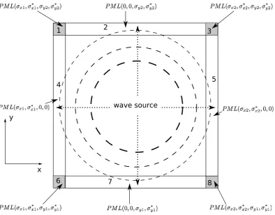
2.8 Structure of a 2D PML . . . 52

(13)

LIST OF FIGURES

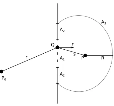
2.10 Geometric arrangements for evaluating RS diffraction formula . . 56

3.1 Planar Waveguide Schematics . . . 58

3.2 Planar Field profiles at XZ plane for TE . . . 59

3.3 Propagation angle and the corresponding field profiles . . . 60

3.4 Mode angles vs normalised height (d/λ) of a Planar waveguide, N A= 0.15 . . . 64

3.5 qd/2 vs hd/2 curves for the detrimental equation of planar struc-ture, d= 2µm, N A= 0.15 . . . 67

3.6 FDTD simulations of the incident angles and the supported modes 67 3.7 Planar Waveguide with lossy cladding . . . 69

3.8 Lossy Guide Parameters . . . 71

3.9 Confinement factor and Loss vs tanδ . . . 72

3.10 Field along guide dimension for lossy cladding . . . 73

3.11 Field profile for lossy cladding . . . 73

3.12 Sinc function plot . . . 74

3.13 Point source in single mode guide . . . 75

3.14 Point source in a multi-mode guide . . . 76

3.15 Plane wave in a multimode guide . . . 77

3.16 Plane wave incident at an angle to excite the higher order modes . 77 3.17 Mode input - mode output; multimode . . . 78

3.18 Gaussian input - mode output; multimode guide . . . 79

3.19 Lossy Mode input - mode output . . . 80

3.20 Rectangular guide - mode along dimension; planar guide field along dimension . . . 82

3.21 nef f changes with b/a ratio; NA=0.15, λ= 550 nm . . . 82

3.22 Sun spectra on the Earth surface source: . . . 83

3.23 Visible spectrum source: . . . 84

3.24 Approximating irregular geometries with FE and FD based methods 85 3.25 Examples of approximating some complicated geometries in FE based mesh (Burkardt [2011]) . . . 86

(14)

LIST OF FIGURES

3.27 The first and the second modes of the rectangular waveguide with fields along the axis . . . 88

3.28 Circular Optical Waveguide structure . . . 89

3.29 First 20 modes of a Circular waveguide, core diameter 2µm, NA=0.15 90

3.30 Comparisons of the field profile of mode 1 and mode 4 of a circular optical waveguide . . . 91

3.31 Hexagonal Optical Waveguide Structures . . . 92

3.32 First 20 modes of a Hexagonal waveguide, side-side distance 2µm, NA=0.15 . . . 93

3.33 First 20 modes of a Elliptical waveguide, major axis 2.2µm, minor axis 1.8µm, NA=0.15 . . . 94

3.34 Guide having irregular cross-section Structure . . . 95

3.35 First 20 modes of a irregular cross-section waveguide, approximate dimension 2µm NA=0.15 . . . 95

3.36 Structures and the propagation characteristics of the first and the second modes for the first mode of Rectangular, Hexagonal, Cir-cular and irregular cross-sections with similar dimensions . . . 96

3.37 Hx

32 field profiles for a rectangular waveguide . . . 97

3.38 Different types of symmetries present in the field profiles of a Hexagonal guide . . . 97

4.1 Schematics of a planar waveguide . . . 100

4.2 Schematic diagram of the XY plane cross-section of a rectangular guide with lossless core and lossy cladding materials . . . 101

4.3 Normalised nef f vs normalised frequency of Hx11 mode (v) for a

2_×2µm rectangular waveguide for different tanδ, ncore = 1.347,

ncladding = 1.339 . . . 102

4.4 Effective index vs Loss tangent for Rectangular guide with 2µmX2

µm dimension, ncore = 1.347, ncladding = 1.339, λ = 550 nm FEM

simulation . . . 103

(15)

LIST OF FIGURES

4.6 Loss vs Guide Width (d) for Different Loss Tangents,ncore = 1.347,

ncladding = 1.339, λ = 550 nm . . . 105

4.7 Real nef f vs tanδ for different wavelengths for a 2µm×2µm

rect-angular waveguide, ncore= 1.347, ncladding = 1.339 . . . 106

4.8 Imaginary nef f vs tanδ, for a 2 µm×2µm rectangular waveguide,

ncore= 1.347, ncladding = 1.339 at different wavelengths . . . 107

4.9 Hx along dimension for Different Loss Tangents, for a 2µm×2µm

rectangular waveguide,ncore= 1.347, ncladding = 1.339 . . . 108

4.10 Field intensity along guide width for Rectangular guide with 2

µm×2 µm dimension . . . 109

4.11 Dispersion vs Frequency for a 2µm Rectangular guide for different tan δ . . . 110

4.12 Effective index for the first 2 modes with different loss tangents . 112

4.13 Confinement factor and Loss vs tanδ . . . 113

4.14 Effective index for the first 2 modes with different Guide separation,d115

4.15 Field intensities of a Rectangular Guide along Guide axis for Dif-ferent Per, d; loss-less cladding is considered . . . 117

4.16 Mode 2 cutoff comparison with single guide and periodic guides with different periodicity . . . 118

4.17 Schematics of a Directional Coupler . . . 119

4.18 Coupling Length of a Directional Coupler with lossy cladding . . 119

4.19 Schematics and the Refractive index (n) profiles of a W-fibre like waveguide . . . 120

4.20 Dispersion for Circular insect ommatidium with 3 layers and scat-tering boundary condition . . . 121

4.21 Dispersion for Circular insect ommatidium with 3 layers and Dirich-let boundary condition . . . 122

4.22 Dispersion for Circular insect ommatidium with 3 layers and Peri-odic boundary condition . . . 122

4.23 Cross section of a Drosophila melanogaster Ommatidium source: Photobiology . . . 124

4.24 Impact of diffraction on the field profile at the Rhabdom entrance 124

(16)

LIST OF FIGURES

4.26 FDTD simulation of insect ommatidium, 3 layers, conductivity

σ = 5000 for the first cladding, the second cladding is loss-less . . 126

4.27 FDTD simulation of insect ommatidium, 3 layers, conductivity

σ = 0 for the first cladding,σ = 5000 for the second cladding . . . 126

4.28 FDTD simulation of insect ommatidium, 3 layers, loss-less . . . . 127

4.29 Schematics of the position of the point source and the excited modes in rhabdom of compound insect eye . . . 128

(17)

List of Tables

1.1 Permittivities of some Biological Tissues at 100 GHz . . . 11

3.1 Relationship between confinement factor and nef f . . . 60

3.2 TE and TE modes with their respective field components . . . 61

(18)

List of Symbols and Abbreviations

Symbol Description

EM Electromagnetic

FEM Finite Element Method

RS Rayleigh-Somerfeld Diffraction Integral FDTD Finite Difference Time Domain

BPM Beam Propagation Method

TE Transverse Electric Polarised Mode TM Transverse Magnetic Polarised Mode

0 Real part of the Permittivity

00 _{Imaginary part of the Permittivity}

nef f Effective Index

tanδ Loss Tangent

n0 _{Real part of the Refractive Index}

(19)

Chapter 1 Introduction

It is of considerable interest and importance about the Electromagnetic Wave (EM) propagation through the biological media, and over the last few decades several landmark studies such as by Johnson and Guy [1972], Sebbah [2012], Ishimaru [1977], have conducted to assess the various aspects of the propagation characteristics of EM radiation and interactions. In the rise of the applications in wireless communications to evaluate the impacts of EM wave, especially in Microwave range, on various human tissue have been studied in great details A Peyman, S Holden[2000]. In the advent of interest in Vision Research, Biophoton-ics Research, Biomedical Imaging, OptoelectronBiophoton-ics Retinal Prosthesis Systems, Computer Vision and some other similar fields have encouraged the researchers to study interactions of EM wave in the other frequency ranges, especially in the Visible spectrum and IR wavelengths. EM wave penetration, reflection, refrac-tion, absorprefrac-tion, and scattering through various biological structures have been studied by various research groups over a wide frequency range. The advances in optical waveguide technologies have seen a rapid development in methods and techniques in analysing EM wave-material interactions. It has been reported that some biological micro-structures can work as waveguides for Visible and IR radi-ations. Evolution over millions of years has perfected the engineering designs of some of these structures to a point where it is very likely that studying them in greater details might provide us with some novel designs as well as give us deeper insights into the functionalities of these systems.

(20)

questions remained unexplained. A recent study by Franze et al. [2007] showed that the Glial cells of Human retina act as an optical waveguide that helps to increase the visual acuity, which earlier was considered has no impacts on vi-sion other than providing the mechanical support to the retinal layers. There is still an ongoing debate amongst the researchers whether the Glial cells are acting as optical waveguides or not. Unavailability of the detailed material pro-files of the system makes it tough to draw a well-accepted conclusion. Retinal photoreceptors were shown by Biernson and Kinsley [1965] to have waveguide properties. However, the relationship between the Glial cells waveguide and the photoreceptor waveguide has not been established to date. Rhabdom present in the Ommatidium of Insect compound eye was shown by Stavenga[1975] to have waveguide properties. The supported mode shapes of these structures and the roles played by them in vision have not been studied in great details.

The materials used in various waveguide devices are mostly have known ma-terial properties with homogeneous mama-terial profiles. Most of the mama-terials such as SiO2, Silicon, Ge and Quartz have known refractive indices and loss values

over a broad range of operating frequencies. The loss values of these materials are usually minuscule (tanδ _≈ 10−4 _{or less) and the propagation}

(21)

the optical waveguides and its impact on the visual process is not available in the literature. It is thus worth studying the biological waveguide structures in visible frequencies and their relationship with the Diffraction present in these systems. The focus of this thesis will be on investigating in determining the impacts of material loss present in the biological structures on their propagation character-istics and relate the presence of diffraction with it. As a test case, Ommatidium of insect (Drosophila melanogaster, Fruit fly (Fig. 1.1)) and the Glial cells of the human retina will be considered.

1.1 Background

1.1.1 Insect eye - Compound eye

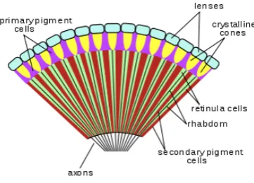
Most of the insect species have a compound eye. A compound eye of most of the insects is composed of Ommatidium, the basic building blocks of the system. Figure 1.2 shows the cross-section of a Drosophila Melanogaster Compound eye. Each ommatidium, as shown in Fig. 1.3 is composed of a lens, crystalline cone, rhabdom and at the end of the rhabdom the photoreceptors are located. The Rhabdom is surrounded by layers containing pigments that act as an absorbing medium for light. Light is focused by the lens and the crystalline cone on the rhabdom and then the light has to be guided by the rhabdom to be absorbed by the photoreceptors. It was shown in some studies by Neumann[2002] and Land [1997] that they can work as a light guide as the refractive index of the rhabdom was found to be higher than that of it surrounding materials. These studies considered the rhabdom and its surrounding materials to be loss-less, which is not accurate.

(22)

[image:22.595.217.402.141.285.2]

Figure 1.1: Image of a Drosophila, source: en.wikipedia.org

Figure 1.2: Insect Compound Eye Cross-section source: en.wikipedia.org

[image:22.595.218.399.355.485.2]

(23)

1.1.2 Absorbing surroundings of the Rhabdom

It is believed that each rhabdom is surrounded by light absorbing layers, pigment layers so that any light tries to escape from the rhabdom can be absorbed by them. It is also believed that the long and short pigment layers, surrounding the Rhabdom as shown in Fig. 1.3 absorbs light that tries to escape the Rhabdom, that means the surrounding materials cannot be loss-less as were considered by the previous studies.

1.1.3 Mammal eye

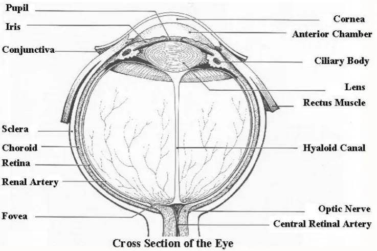
[image:23.595.125.494.406.651.2]

A typical Mammal eye cross-section is shown in Fig. 1.4. The light passes through the cornea, the anterior chamber filled with Aqueous Humor, Pupil, Lens, and the Interior chamber filled with Vitreous Humor to reach the photosensitive layer known as the Retina.

Figure 1.4: A typical Mammal Eye, source: wikimedia commons

(24)

monochro-matic vision in dim light) are located at the back of the Retinal layers just before the pigment cell layer. The light must pass through the different layers of the retina, such as Horizontal cells, Bipolar Cells, Amacrine Cells and Ganglion Cells to reach the photoreceptors. Photoreceptor cells converts the light into elec-tricity and then the electric current is transferred by the Horizontal, Bipolar and Amacrine cells to the Ganglion cells. Ganglion cells are in fact the neurons whose axons form the optic nerve that transfers the visual information acquired by the Retina to Brain for further processing and interpretations.

The seemingly inverted design of the Mammal retina had been a riddle for the vision science researchers as the photoreceptors present at the back of the Retinal layers receive optical stimulations that are passing through the different layer and is expected to suffer severely scattering by them. Muller Cell or the Glial cells, as shown in Fig. 1.7, present in the Retina that spans from the Ganglion cell layer up to the photoreceptor layer were previously considered to provide structural support to the Retinal different layers. It was shown by Reichenbach et al.[2012] that the glial cells work as a light guide between the top surface and the photoreceptor layer and, in fact, enhances the visual acuity to some extent. The Glial cell matrix thus transfers the image information projected by the Eye-Lens on the top surface of the Retina to the Photoreceptor layer, where it is being guided and absorbed by the Photoreceptors. The presence of Bragg grating like optical filter makes the cones sensitive to a certain colour of lights and makes the rods exhibit a broadband response.

2 Background

the succeeding secondary and tertiary neurons of the retina (Rodieck, 1973; Masland, 2001). In general, rods and cones synaptically transmit the biochemical message to the bipolar cells that in turn trigger the retinal ganglion cells. Thereby, different types of horizontally oriented amacrine and horizontal cells modify the serial information flow by lateral inhibition processes. Finally, the ganglion cells generate action potentials that run along their axons at the innermost layer of the retina. The optic nerve collects the axons of all ganglions and delivers the information to the visual cortex in the brain (Figure 2.9 a).

Figure 2.8: The retinal tissue in the eye. (a) The retina is a thin cell layer that converts images of the environment into a visual information which finally can be perceived by the brain. (b) Photograph of a freshly isolated retina in aqueous solution. Images adapted from Ignacio Icke, Wikimedia Commons and from Franze (2007). Scale bar 200µm.

Under the microscope, the retina shows a distinct stratified structure where the different morphological elements of the retinal cells are well-organized in separate layers (Figure 2.9 a; Rodieck, 1973). The inner and outer segments of the photoreceptor cells form the photoreceptor segment layer (PRS) while their cell bodies are densely packed in the outer nuclear layer (ONL). Cellular processes and synaptic terminals of rod (spherules), cone (pedicles), bipolar and horizontal cells are located in the following outer plexiform layer (OPL). All layers containing substructures of the receptor cells belong to the so-called outer part of the retina which again reflects the positioning away from the incoming light. Similar to the outer part, the inner retina includes an inner nuclear (INL) and an inner plexiform layer (IPL) formed by cellular structures of the downstreamed neurons. The cell bodies of the ganglion cells are located in the ganglion cell layer (GCL) and their axons in the nerve fiber layer (NFL). In addition to the neurons, the retina contains also non-neuronal glial cells, the second cell type of the nervous tissue. The main glial cells of the retina, the Müller cells, span the entire tissue from the inner retinal surface towards

Figure 1.5: Retina Layers and Cross-sectionReichenbach et al. [2012]

(25)

Figure 1.6: Photoreceptors in Mammal Retina, source: www.bioteaching.com

uc

tion

e

gr

ee

k

w

or

d

“⁄

ÿ–

an

d

si

m

pl

y

m

ean

s

gl

ue

(Vi

rc

ho

w

,

1856)

.

He

nc

e,

M

ül

le

r

ce

lls

n

gl

ial

ce

lls

of

th

e

re

tin

a

re

m

ai

ne

d

vi

rt

ual

ly

un

ex

pl

or

ed

fr

om

th

ei

r

fir

st

de

sc

rip

tion

G

er

m

an

at

om

is

t

He

in

ric

h

M

ül

le

r

in

1851

un

til

th

e

en

d

of

th

e

20t

h

ce

nt

ur

y

w

he

n

sl

y

im

pr

ov

in

g

m

et

ho

ds

in

ce

ll

bi

ol

ogy

pr

om

ot

ed

a

re

nai

ss

an

ce

of

gl

ia

re

se

ar

ch

r,

1851;

K

an

de

le

t

al

.,

1999)

.

Ne

ve

rt

he

le

ss

,al

re

ad

y

M

ül

le

r’s

de

sc

rip

tion

of

“r

ad

ia

l

s

sp

an

ni

ng

th

e

en

tir

e

th

ickn

es

s

of

th

e

ret

in

a”

poi

nt

s

ou

t

th

e

fa

vor

ab

le

m

or

ph

ol

ogy

le

r

gl

ial

ce

lls

to

tr

an

sp

or

t

ligh

t

th

rou

gh

th

e

tis

su

e

to

th

e

re

ce

pt

or

ce

lls

(F

igu

re

1. 1)

.

1. 1:

He

in

ric

h

M

ül

le

r’s

or

igi

nal

dr

aw

in

g

of

M

ül

le

r

rad

ial

gl

ial

ce

lls

.

(M

ül

le

r,

1851)

.

g

th

e

pas

t

de

cad

e,

se

ve

ral

ex

pe

rim

en

ts

ha

ve

sh

ow

n

a

par

tic

ul

ar

ligh

t

pe

rm

eab

ili

ty

le

r

ce

lls

w

hi

ch

se

ts

th

em

ap

ar

t

fr

om

th

e

op

tic

al

pr

op

er

tie

s

of

th

ei

r

su

rr

ou

nd

in

g

ne

u-ran

ze

et

al

.,

2007)

.

Tu

rn

in

g

to

th

e

qu

es

tion

of

th

e

un

de

rly

in

g

ph

ys

ic

al

pr

in

ci

pl

e,

it

e

st

rik

in

g

si

m

ilar

ity

w

ith

fib

er

op

tic

cab

le

s

in

a

pl

at

e

w

hi

ch

le

d

sc

ie

nt

is

ts

to

as

su

m

e

ül

le

r

ce

lls

ac

t

as

liv

in

g

w

av

e

gu

id

es

w

ith

in

th

e

re

tin

al

tis

su

e.

Ho

w

ev

er

,n

on

e

of

th

e

ap

pr

oac

he

s

fu

lfi

lle

d

al

lr

eq

ui

re

m

en

ts

to

pr

ov

e

th

is

hy

pot

he

si

s.

T

hi

s

al

so

in

cl

ud

es

rim

en

t

fr

om

Fr

an

ze

et

al

.(

2007)

w

he

re

it

w

as

sh

ow

n

th

at

in

di

vi

du

al

M

ül

le

r

ce

lls

,

be

tw

ee

n

tw

o

gl

as

s

fib

er

s

of

a

m

od

ifi

ed

du

al

-b

eam

las

er

tr

ap

,ar

e

ab

le

to

gu

id

e

th

e

g

ligh

t

fr

om

an

in

pu

t

to

an

op

pos

in

g

ou

tp

ut

fib

er

.

G

en

er

al

ly

,i

sol

at

ed

ce

lls

em

be

d-in

hom

oge

ne

ou

s

flu

id

s

do

not

ex

pe

rie

nc

e

th

e

com

pl

ex

op

tic

al

lan

ds

cap

e

of

th

ei

r

en

vi

ron

m

en

tw

hi

ch

in

tu

rn

con

si

de

rab

ly

aff

ec

ts

th

ei

r

op

tic

be

ha

vi

or

.

In

par

tic

ul

ar

,

gu

id

in

g

m

ec

han

is

m

of

a

ce

ll

w

ou

ld

not

on

ly

de

pe

nd

on

th

e

op

tic

al

pr

op

er

tie

s

of

th

e

Figure 1.7: Retinal Glial or Muller Cell, Original Drawing by MullerM¨uller[1851]

(26)

1.1.4 Lossy surroundings of the Glial cells

Photocurrent goes in the upward direction through the Human retina, indicating the presence of finite conductivities of the material, thereby lossy for EM wave. The photoreceptors are surrounded by lossy materials as well. Freshly dissected retina in aqueous solution, as shown in Fig. 1.5, shows that it is not transparent, in contrast to the previous belief that the retina is mostly transparent in the visible spectrum. So, the Glial cells are providing a safe passage for the light through the seemingly non-transparent Retinal layers and it can be concluded that the Glial cell surroundings are lossy in visible frequencies.

1.1.5 Diffraction in the visual systems

Diffraction occurs when a wave encounters an object or a finite aperture. In clas-sical physics, the phenomenon of diffraction can be described as the interference of waves according to Huygens-Fresnel principle (Papas [2014]). According to this principle, each point on the wavefront acts as a new point source.

d a

a

p

ertu

re

sc

ree

n

in

ten

si

ty

p

ro

fi

le

o

n

th

e

sc

ree

n

w

a

v

e

so

u

rc

e

Figure 1.8: Schematics of a single slit diffraction

(27)

When the wave encounters the aperture, each point on the aperture now acts as a new wave source and they interfere with each other as they propagate.

On the screen, the waves from different points reach with different phases, and at some point when the wavefronts are in phase, constructive interference produces higher intensities, where at some other points the destructive interfer-ence produces lower intensities. A typical intensity profile on the screen is shown on the right-hand side of Fig. 1.8.

The intensity profiles generated due to diffraction can be obtained from the scalar solution of the Helmholtz wave equation. There are several methods avail-able in the literature to compute the diffraction profiles, i.e. Kirchoff’s Diffraction Integral Marchand and Wolf [1966], Rayleigh-Sommerfeld Diffraction Integral Osterberg and Smith [1961], Fresnel’s Diffraction IntegralMendlovic et al. [1997], Fraunhofer’s Diffraction IntegralMendlovic et al.[1997], etc. In diffraction theory, the terms ‘near-field’ and ‘far-field’ are used that can be described by Fresnel’s distance to characterise the properties of diffraction. The Fresnel’s distance is given as,

df =

2D2

λ (1.1)

where, df is the Fresnel’s distance, Dis the aperture size, and λ is the operating

wavelength. ‘Near-field’ refers to the region where the distance is less than df,

the region with distance higher than df refers to the ‘far-field’.

(28)

Due to the presence of finite apertures in the visual systems, the quality of the image produced by them are limited by diffraction. The lens present at the beginning of the insect ommatidium and the finite size of the pupil present in mammal eye act as a finite aperture and produce diffraction. Figure 1.9 shows the impact of Diffraction by a finite aperture (For the insect Ommatidium the Lens, for the Mammal eye the pupil) produces airy patterns for a point source.

1.1.6 Challenges in modelling biological tissue

Treatment of biological tissue mathematically is a challenging task. Unlike the dielectrics, where no moving charge is present thereby no conduction, biological tissues can conduct electricity. Although they can conduct electricity, the charge carriers are not electrons or holes like metals and semiconductors, but ions are the charge carriers.

Figure 1.10: Electron Microscope Image of Biological Tissue, Cells

(29)

char-acteristics than that of a dead tissue. Incorporating the impacts of the presence of metabolism is a difficult task. The biological tissues can be considered as lossy dielectrics having finite conductivities mathematically to work with the Maxwell’s equations. As long as the conductivity is not as high as good conductors, the assumptions should produce reasonably accurate results. Figure 1.10 (source: en.wikipedia.org) shows the electron microscope image of a typical biological tis-sue that shows that the structure is highly inhomogeneous and full of scattering particles.

Table 1.1 (source: http://niremf.ifac.cnr.it/) displays the material properties of some of the biological tissues at 100 GHz frequency that shows that at this fre-quency most of the materials are lossy. Here0 is the real part of the permittivity of the material and tanδ = 000 is the loss tangent of the material where 00 is the

imaginary part of the material permittivity. For the visible range of frequencies, most of these tissues are opaque thus highly lossy, some of the tissues such as Retina is considered to be loss-less at visible frequencies, that is why the exact values of losses present are not available in the literature.

Table 1.1: Permittivities of some Biological Tissues at 100 GHz

Specimen 0 _tan_δ

(30)

1.1.7 Mathematical treatments for lossy medium

The absorbing material can be considered as a lossy dielectric having a permit-tivity of = r +ji, where r and i are the real and imaginary parts of the

complex permittivity . For a lossless dielectric material i → 0. Here the

di-electric and conduction losses both are combined into i (Ramo et al. [2008]).

In this thesis, the notations r = 0 and i = 00 have been used, and the

simi-lar notations for the refractive indices (n) have also been used. As long as the material under consideration is not metal or plasma, the treatment of losses in this manner produces results within an acceptable level. The refractive index is given by n =√ =nr+jni, where nr and ni are the real and imaginary parts

of the refractive index. For most of the structures found in biological tissue the imaginary part of the refractive index ni are not available in the literature at

optical frequencies. The impacts of losses for these structures has largely been ignored.

Unfortunately, the previous researchers did not pay sufficient attention to the fact that the loss of the material could be (of any use) valuable in characterising their optical properties of these biological structures. That might be the reason the imaginary parts of the refractive indices are so scarce while the real parts are often available in the literature. The presence of loss in the materials of a light guide can change the propagation characteristics to a great extent. It is thus worth investigating the impacts of the material losses of biological structures on the propagation characteristics.

As the imaginary parts of the refractive indices are not available, the compu-tational analysis can be carried out with a range of assumed values for the ni.

nr of the different components of rhabdom of Drosophila, Human Glial cell and

Photoreceptors of Human retina are however available.

1.1.8 Importance of the structure

(31)

a considerable amount of visual processing. The total amount of energy at their disposal is very limited. For the nocturnal flying insects, the amount of available light is very limited as well.

Despite having all these limitations of smaller available energy, lower computa-tional power, lower available light (nocturnal); their visual system must perform very well to survive in nature. A Huge number of well-survived insect species suggests that they are performing very well indeed. The image capturing and projection system (Insect compound eye) must be producing acceptable qual-ity images for the accurate representation of the visual scene, provide sufficient information for motion detection, navigation and tracking. Unavailability of a high-performance processing unit behind the eye imposes the responsibility on the physical structure of the eye so that it reduces the burden on the processing to a great extent and less amount of further processing is required. Hence, the structure of their eye must be playing a very vital role in insect’s visual system.

1.1.9 Previous studies on these structures

The refractive indices of the interior materials of Rhabdom, Glial cells and Pho-toreceptors in the retina, are higher than their surrounding materials. Hence, all these structures can guide EM wave and some studies Land [1997],Neumann [2002] found that these structures can guide light in the visible spectrum.

(32)

1.2 Overlooked problems

1.2.1 Presence of biological optical waveguide

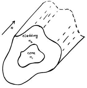
[image:32.595.171.453.268.555.2]

A medium (core) can act as a light guide if it is embedded in another medium (cladding) having a lower value of refractive index. Light is being guided by the inner material if the condition ncore > ncladding is satisfied.

Figure 1.11: Optical waveguide

where, n1 and n2 are as shown in Fig. 1.11. If the incident angle is more

than the critical angle, then the light or the electromagnetic wave in medium 1 experiences total internal reflection and unable to escape the core material, thereby guided in the core material. By using Snell’s law the critical angle, θc is

defined as,

θc =sin−1

n1

n2

(33)

refracted ray medium 1

medium 2

Figure 1.12: Snell’s law

For a light guide, V = πd_λ pn2

1−n22, if n1 > n2, n1 is core refractive index,

n2 is cladding refractive index,d is the diameter of the core, V is the normalised

frequency, V _≤ 2.405 ensures single mode condition Senior [1992], it has been found that for the other waveguide types the value is around 2.4. Any material surrounded by a lower index material exhibits properties similar to the waveguide for EM wave.

(34)

1.2.2 Impacts of lossy surroundings

Propagation characteristics would be different from that of lossless case Balanis [1989]. Potentially it could answer some of the unanswered riddles in the visual system.

1.2.3 Impacts of neighbouring structures

The previous studies Neumann [2002] treated the structures as that of a single core optical fibre, where it has been considered that the cladding material is extended to infinity. In reality, each of the photo guides is embedded into a photo-guide matrix. The propagation characteristics of a single guide are not only determined by its structure and the material profiles but also the surrounding structures present. These photoguide matrix structures are very similar to that of multi-core optical fibres Nagashima et al. [2013]. By choosing appropriate boundary conditions, we can address the presence of the surrounding guides.

1.2.4 W-fibre structure in insect rhabdom

Impacts of a 3-layer structure of rhabdom are yet to be explored - dispersion flattening effects, cutoff wavelength shift due to the multi-layered structure needs to be addressed.

1.2.5 Limitations of RAY optics based models

Some RAY optics based models of Human eye are presented by Navarro et al. [1986], Neumann [2002], Navarro [2009], and Talu [2011]. At smaller retinal ec-centricities the impacts of diffraction and spherical aberration can be determined, but the paraxial approximation based calculations cannot be used for larger ec-centricities, at the peripheral regions. What intensity profile is present at the guide entrance cannot be explained by these models that are necessary for modal analysis. RAY optics-based methods use the paraxial approximation, makes them useful in determining intensity profiles in the Fraunhofer’s zone or far field.

(35)

cases. Even if we can determine the intensity profiles - would only valid for the central 1-5 degrees in the visual field. If we go beyond that angle, the image screen becomes curved.

RAY optics-based methods give us acceptable results when the propagation distance is much large compared to the wavelength (r >> λ) and the propa-gation angle remains small (paraxial approximation). Although, apart from the foveal region of human eye, large angles are required to address the peripheral retina, distance between the lens and the retina that is approximately 22 mm, makes it suitable for the RAY optics based analysis, at the same time makes it computationally too expensive to employ any Time Domain-based numerical methods.

1.2.6 Point source position and excited modes

A point source directly ahead of the ommatidium should excite the fundamental mode for the rhabdom. The other point sources in the surroundings would try to excite the higher order modes that should be blocked by the ommatidium unit to preserve the clarity of the transferred image by the ommatidium mosaic. The exact mechanism of how these higher order modes are being attenuated highly needs more in-depth study.

For the diurnal insects, it has been found that they have apposition eye, where the nocturnal insects most commonly have superposition eye. In superposition eye, each rhabdom takes excitations not only from the points directly ahead of it but also excitations from the neighbouring points. As the light from the neighbouring points fall at a higher angle, they would excite higher order modes in them. Angle dependence of the modes is necessary but not was not explored in details in the previous studies.

1.3 Aim of the Thesis

(36)

Retina) in the visible spectrum. The study will characterize not only the indi-vidual waveguides but also the impacts of the surrounding waveguides on the characteristics. A link between the RAY optics based analysis and the modal analysis of the optical waveguides will be studied. The angle dependence of the excited optical mode within a waveguide and their consequences will be studies in greater details.

1.4 Tools Available

1.4.1 Analytical solution

The scalar solution of Helmholtz equation can be obtained as presented by Bal-anis [1989]. As the solution is scalar, the phase information cannot be obtained. As human eye is not phase sensitive, so a scalar solution can be acceptable. All these methods work well for regular geometries. Working with the inhomoge-neous material is tough. This solution is suitable for large propagation distance. Fraunhofer’s diffraction integral works in the Fraunhofer’s (Manakov [1973]) re-gion, for the far field. This method is not suitable for large propagation angles. Fresnel’s diffraction integral works well at near field with Fresnel’s approximation. However, it is not suitable for the large angles. Kirchhoff’s diffraction integral works well for the large angle, but the formula is mathematically inconsistent. The Rayleigh-Sommerfeld diffraction integral(RS) formula is suitable for large propagation angles, and the integral is mathematically consistent. As the analy-sis of biological structures requires analyanaly-sis over a large propagation angles, the Kirchhoff’s diffraction integral or the RS diffraction integral can be used.

1.4.2 Ray Optics

(37)

However, for a brief insight into the system, it might be helpful but not suitable for analysis at sub-wavelength scale with irregularities.

1.4.3 Numerical solutions of Maxwell’s equations

1.4.3.1 Finite Difference based modal solutions

Regular grids used in this method makes the method not suitable where irregular boundaries are present. The inhomogeneous material profile can be handled with this method, and it is computationally less expensive than the finite element based methods. However, the Cartesian grids used to approximate irregular boundaries would produce results with higher numerical errors.

1.4.3.2 FEM based modal solutions

Finite element based mode solver, as they can use FE meshes, are excellent at approximating structures with irregular boundaries. Inhomogeneous material profiles can be addressed well, but the 2D FEM considers the structure and the materials to be uniform in the direction of propagation, so a structure that has variations in the direction of propagation is difficult to analyse using this method. If it is required to obtain the mode profile at a 2D cross-section, this method can provide us with reasonably accurate results although computationally it is more expensive than the FD based method.

1.4.3.3 BPM

(38)

wavelength. The main features of the BPM are that the electromagnetic fields are Fourier transformed about the direction normal to that of light propagation and that a stepwise method is used for successively calculating the electromagnetic field along the axial direction.

In the BPM, the optical field is transported within one propagation step, from the transverse plane at the longitudinal coordinate z to the transverse plane at

z+ ∆z. Calculations are performed, to relate the optical fields at the input and the output planes, which are based on the assumption that the dielectric profile within one step, ∆z, remains unchanged Nolting and M¨arz[1995]. As the optical field propagates through the medium, it is subject to diffraction due to its wave nature, and the light rays of the wave experience a certain amount of phase shift, depending on their x andy positions. The above influence can be applied one at a time, provided that the space along the path be subdivided into tiny sections, ∆z. By doing so, the continuous medium can then be realized as a series of lenses separated by short sections of homogeneous space, where the contribution of the lenses in the phase shift is expressed in the solution of the wave equation. For computational purposes, the wave between the lenses can be decomposed into its spectrum of plane waves by applying a Fast Fourier Transform (FFT) algorithm, and then it is reconstructed halfway, (∆z/2), before the next lens, by applying the inverse FFT. The above process is repeated for each section along the whole propagation path. The propagation step size ∆z, which must be at most one wavelength of the light beam, must ensure that the contribution of evanescent waves, which are part of the plane wave, is negligible, and that the rays associated with the wave, travel parallel to the z-axis, with minimum phase shift.

(39)

techniques such as the Fresnel approximation Yevick and Hermansson[1989]. Beam Propagation Method (BPM) makes paraxial approximations (although non-paraxial approximation is possible as well), so it is not suitable for an abrupt change in field envelopes. It can address inhomogeneous material profiles in the direction of propagation as well as in the cross-section but steps. Computationally the method is much more expensive than the modal analysis but cheaper than the time domain methods. BPM is unable to address reflections from the interfaces, although its Bi-directional variation can do that, more expensive computationally.

1.4.3.4 FETD

(40)

1.4.3.5 FDTD

In 1966 Yee et al. [1966] proposed a finite difference based technique to solve Maxwell’s equations over time to analyze time evolutions of Electromagnetic waves. His proposed method is widely known as the Finite Difference Time Do-main (FDTD) method. The method uses a rectangular Cartesian grid in 2D and cuboid grid in 3D to discretize the computational domain and solves Maxwell’s equations over the domain.

The method is numerically stable and robust. Explicit formulation and the data-parallel nature of the method makes it very fast making it computationally less expensive. For a computational domain with inhomogeneous material profiles and with a geometry that can produce strong reflections, FDTD method has been found to be very useful in dealing with it. Scattering, if present in the system, can be analyzed by using this method. So, for analyzing biological structures, where the inhomogeneous material and irregular structures can produce strong reflections and scattering, the FDTD method can be very useful in analyzing the characteristics of such systems. The method has, however, some disadvantages when deployed in analyzing the biological structures. Due to the use of rectangu-lar or cuboid grids in representing the structures, the method approximates the curved of slanted boundaries with stair-casing, which in turn produces numerical errors. The biological structures, as we know, are most of the cases irregular or semi-irregular in nature; that is why the method is not the optimum choice for biological applications. The method is not suitable for simulations over large dis-tances (d >> λ) due to numerical dispersions. So, this method can be considered as the candidate by which the time domain evolution can be analyzed for the irregular structures with the irregular material profiles with less computational power sacrificing the numerical errors due to the FD grid.

1.5 Methodology and Study steps

(41)

propa-gation and guidance through biological optical waveguides having lossy materials. Mode profiles, dispersion characteristics, impacts of losses on various character-istics will be explored. The study will start with a simple structure and move towards a complicated biological structure.

1.5.1 Planar structure

As a beginning, the study will be focused on a planar optical waveguide. The reason behind choosing a planar waveguide is that the Analytic modal solution is available for such waveguides that can be used to benchmark the algorithms. As a planar structure can be considered as a limiting case of a rectangular structure, the characteristics found by analysing a planar structure can be extrapolated to get an approximate idea of the similar characteristics of the rectangular structure. The study on this structure will focus on the following topics,

• Theoretical derivations for modal solutions

• Obtain Mode profiles

• FDTD simulations of these structures

1.5.2 3D structures

Propagation characteristics of 3D optical waveguides with lossy surrounding will then be studied extending the knowledge acquired from planar waveguide studies. The 3D waveguides with the following cross-sections will be explored,

• Rectangular waveguides

• Circular waveguides

• Hexagonal waveguides

• Irregular shaped waveguides

Two types of layered structures are studied

(42)

• 3 layers

The following boundary conditions for each of these case will be tried,

• Dirichlet boundary condition - field zero at the computational domain

• PML boundary condition

• Periodic boundary conditions - considering the array of guides

1.5.3 Test cases

After analysing different types of optical waveguides with various parameters, the study will focus on analysing two biological structures that are known to work as optical waveguides. The first case being the Rhabdom of the Ommatidium of the compound eye of the Drosophila Melanogaster (Fruit Fly), and the second being the Glial cells of the Retina of Human Eye.

1.5.3.1 Drosophila Melanogaster (Fruit fly) Compound Eye

The study will analyse the Rhabdom on the following key points,

• Mode profiles

• Single mode operating wavelength range

• 2 layers and 3 layers

• Periodic boundary conditions and its impact

• Coupling amongst the surrounding guides

• How loss is exploited

1.5.3.2 Glial cells of Human Retina

The characteristics of the Glial cells of Human Retina will be analysed focusing on the following points,

(43)

• Directional sensitivity - leading to an explanation of Stiles-Crawford effect of first and second kind

• Impacts of lossy surroundings

1.5.3.3 Integrated Diffraction integral and Modal solutions

Rayleigh-Sommerfeld diffraction integral is used to determine the field intensity profile at the glial cell entrance of the retina of the human eye. The field profile at the entry of the rhabdom of the Ommatidium of insects’ compound eyes is determined. Field profiles found from the modal solutions are compared with the diffraction patterns. FDTD is used to assess the propagation characteristics of such field profiles. The relationship between the field profiles found by the RS diffraction integral and field patterns for the supported mode profiles of these guides will be analysed.

The following topics are included in the step by step study,

1. RS diffraction integral to evaluate the field profiles from the pupil to the glial cell entrance of Human eye; Lens to rhabdom entrance of the compound eye of insect (Drosophila).

2. Ray optics to determine the angle of incidents over the retinal eccentricities.

3. Theoretical derivations for planar structures with lossy medium and their numerical evaluations.

4. FEM to determine the mode profiles for rectangular, square, circular, hexag-onal and irregular shaped guides with as well as without losses.

5. Test cases: Drosophila rhabdom and Glial cells of human retina.

6. Relate the ray optics, RS, FEM and FDTD findings.

7. Impacts of loss on mode profiles, dispersion and cutoff wavelength.

8. Single mode cutoff wavelengths for different structures.

(44)

10. Coupling amongst the neighbouring guides.

11. Stiles-Crawford effect.

1.6 Thesis organization

(45)

Chapter 2 Simulation Environment

2.1 Maxwell’s Equations

The Maxwell’s equations can characterise the propagation of Electromagnetic wave. Maxwell’s equations comprise a set of four electromagnetic field vectors that describe the governing laws of electromagnetic wave propagation. The vec-tors are electric field intensity E (Volts/meter), the magnetic field intensity H

(Amperes/Meter), the electric flux density D (Coulombs/m2_{) and the magnetic}

flux intensity B (Tesla). For a source-free region, time-dependent equations can be expressed in differential and integral forms. In FEM, we formulate the problem as a boundary value problem with a set of differential equations. The differential form of Maxwell’s equations can be given as follows,

∇ ×E+∂B

∂t = 0 (2.1)

∇ ×H− ∂D

∂t = 0 (2.2)

∇.D =ρ (2.3)

(46)

D=E (2.5)

B =µH (2.6)

Here, ρis the electric charge density (Coulombs/m3). The permittivity and the permeability µ of the medium can be given as,

=0r (2.7)

µ=µ0µr (2.8)

where, 0 is the permittivity of the free space (8.854×10−12 Farads/meter), r is

the relative permittivity of the medium, µ0 is the permeability of the free space

(4π_×10−7 _N/_A2_{) and} _µ

r is the relative permeability of the medium. When we

consider a material in optical frequencies another parameter, refractive index n

is very often used that can be expressed in terms of r and µr as follows,

n =√rµr (2.9)

for a non-magnetic material µr = 1, in this case,

n =√r (2.10)

Boundary Conditions

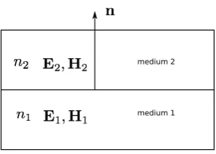
At the material interface between two media, a set of conditions must be met by the field equations, these are known as the boundary conditions. Figure 2.1

shows a structure with two mediums, Medium 1 with a refractive index n1 and

Medium 2 with a refractive indexn2, and the unit normal vector nis the normal

(47)

1. The tangential components of the electric fields must be continuous

n_×(E1−E2) = 0 (2.11)

2. The tangential components of the magnetic fields must be continuous

n×(H1−H2) = 0 (2.12)

3. The normal components of the electric flus density must be continuous

n.(D1−D2) = 0 (2.13)

4. The normal components of the magnetic flux density must be continuous

n.(B1−B2) = 0 (2.14)

If one of the media is a perfect conductor, at the interface the following con-ditions must be met to ensure the continuity of the fields. Such a boundary is known as the electric wall boundary condition.

n_×E= 0 or n.H= 0 (2.15) If one of the media is a perfect magnetic conductor, the magnetic wall boundary condition can be given as,

n_×H= 0 or n.E= 0 (2.16) In analysing optical waveguide devices at the boundary of the waveguide, additional boundary conditions are considered. The boundary conditions are as follows,

Φ = 0 Homogenous Dirichlet (2.17)

(48)

∂Φ

∂n = 0 Homogenous Neuman (2.19)

Here the φ can be the electric or the magnetic field, k is a constant and n is the unit normal to the interface. In Homogeneous Dirichlet the field value at the computational boundary is considered to be 0, in Inhomogeneous Dirichlet it is considered that constant valued field specified by the constantk is present at the border and in Neumann boundary condition considers that the rate of change of the field with respect to the surface normal n is 0.

[image:48.595.224.380.300.411.2]

medium 1 medium 2

Figure 2.1: Boundary between two media having refractive indices n1 and n2, n

being the unit vector normal to the interface

Wave Equation

For an isotropic, loss-less (J = 0, ρ = 0) and non-magnetic (µ =µ0) material

with a permittivity the Maxwell’s equation for the 3-D case can be written as follows,

∇2_E₊_k2_E_{= 0} _(2.20)

∇2_H₊_k2_H_{= 0} _(2.21)

where the k (rad/m) being the wavenumber that is given as,

k =ω√µ0 (2.22)

when =0 (free space), the free space wavenumber k0 is given by,

(49)

Equations2.20 and 2.21 are known as Helmholtz wave equations in 3-D.

2.1.1 Variational Formulation

The finite-element formulation can be based on the variational or Raleigh-Ritz approach. These can be in scalar form, where only one electric or magnetic field component is considered; or in vector form where the electric or magnetic field is expressed in terms of at least two components. Most of the formulations applied to FEM gives us a standard eigenvalue problem of the following form,

[A]_{x_{} −}λ[B]_{x_}= 0 (2.24) where [A] and [B] are real symmetric sparse matrices, and B is positive defi-nite. The eigenvalue λ can be chosen as β2 _or_k2_{, depending on the formulations}

and the eigenvector xrepresents the nodal field values of the finite elements.

2.1.2 Scalar Approximation

The scalar approximation can be applied in the situations where the fields can be describes as TE (Transverse Electric) or TM (Transverse Magnetic) modes. For the quasi-TE modes over a region Ω withExbeing the dominant field component,

the formulation describes by Mabaya et al. [1981] as follows,

L= Z Z Ω " ∂Ex ∂x 2 + ∂Ex ∂y 2

−k2₀n2E_x2+β2E_x2 #

dΩ (2.25)

For the quasi-TM mode with dominant Hx component, the formulation can

be written as follows,

L= Z Z Ω " 1 n2 ∂Hx ∂x 2 + 1 n2 ∂Hx ∂y 2

−k₀2H_x2+ 1

n2β 2_H2

x

#

dΩ (2.26)

2.1.3 Vector Formulation

(50)

cross-section), where all 6 components of the fields (Electric : Ex,Ey andEz; Magnetic

Hx,Hy, andHz) can be present, cannot be analysed by using a scalar formulation.

Although vector Efield based formulations have been used earlier, but the vector

H field based formulation is found to be more suitable for analysing dielectric optical waveguides, because the magnetic field is continuous everywhere, as long as the material is non-magnetic for which µ = µ0, and the natural boundary

conditions correspond to that of an electric wall, therefore no enforced boundary conditions are required. The formulation is as follows,

ω2 =

R

(∇ ×H)∗.ˆ−1_.₍_{∇ ×}_H₎_d_Ω

R

H∗.µ.ˆHdΩ (2.27) here, ω is the angular frequency in radians, Ω is the waveguide cross-section, ˆ

is the permittivity tensor and ˆµis the permeability tensor. In order to obtain a stationary solution for the function in equation 2.27, the expression in minimised with respect to the components Hx, Hy and Hz. This minimization leads to the

matrix eigenvalue equation as of equation2.24, where [A] is a complex Hermitian matrix and [B] is a real symmetric and positive-definite matrix. The eigenvalue

λ is proportional to ω2 _{and the eigenvectors} _{_x_} _{are the} _H _{field values at the}

node points of the elements. The iterative solution starts with an initial guess of the propagation constant β for a given wavelength, equation2.24 is then used to determine a value of the eigenvector _{x_}, the obtained eigenvectors _{x_} is then used to determine a new value for the propagation constant β; the process continues until the values of β and _{x_} converges to a stable state. By choosing different values of the initial guess β, it is possible to find out all the supported modes for a given wavelength. By varying the operating wavelengths, the disper-sion characteristics can be determined. Although the formulation is based on H

fields, by using the coupled Maxwell’s equations, it is possible to calculate the E

field components.

(51)

2.1.4 Natural Boundary Condition

The boundary condition that is automatically satisfied when left free in varia-tional methods is known as the ’natural boundary condition’. The scalar for-mulation of equation 2.25 has the continuity of ∂Ex

∂n as the natural boundary

condition, and equation 2.26has _n12 ∂Hx

∂n as the natural boundary condition. Here,

n is the outward normal unit vector to the interface. The vector formulation in equation 2.27 has n.H = 0 (Electric wall) as the natural boundary condition. Therefore, for conducting guide wall, it is not necessary to enforce any boundary condition as the natural boundary condition is automatically satisfied. However, for a guide with regular geometry, exploiting the boundary condition can lead us with reduced matrix problem size. Proper use of symmetry and boundary condition can be useful in cases where mode degeneration is present.

2.2 Numerical Solution of Maxwell’s equation

For three dimensional waveguides that are more commonly used in today’s pho-tonics systems, the analytical solutions in closed form are not always obtainable. Whenever exact analytical solutions are not available, the approximate solutions are sought. Finite Element Method (FEM) is used in modal analysis of optical waveguides by solving Maxwell’s Equations numerically and FDTD is used to study the time evolution of electromagnetic fields within the waveguides. These two numerical methods and various technical aspects of them are described in the following sections.

2.2.1 Finite Element Method (FEM)

The finite element method tries to solve a complicated problem by replacing it with several simpler ones. The physical problem described by the differential equations are replaced by an appropriate functional J that is the variational formulation for the desired result. The problem can be considered as obtaining the solution of H over a region in the transverse plane satisfying the boundary conditions. The axial dependence is assumed as e−jβz_{, and the discretization is}

(52)

Chapter 2. Numerical Method

the boundary conditions and also the extremum requirement are satisfied. The axial

dependence is assumed in the form e j z_{, and the transverse plane is used for the}

discretisation.

1

2 3 ₄

3

1 2

1

2

3

4 1

2 3

4

Triangle Rectangle

Quadrilateral _{Parallelogram}

Figure 2.3: Finite elements in two-dimension.

2.5.1 Domain Discretisation

The discretisation of the domain into sub-regions (finite elements) is considered as the

initial in the finite element method. The shapes, sizes, number and configurations

of the elements have to be chosen carefully such that the original body or domain is

simulated as closely as possible without increasing the computational e↵ort needed

for the solution. Each element is essentially a simple unit within which the unknown

can be described in a simple manner. There are various types of elements available

for use in finite element formulations. These elements can be defined to be as one,

two and three dimensional elements. When the geometry and material properties can

be described in terms of only one spatial coordinate, then a one-dimensional element

can be used. However, when the configuration and other details of the problem can

be described in terms of two independent spatial coordinates, the two-dimensional

elements shown in Fig. 2.3 can be used. The simplest and indeed the most basic

element typically considered for two-dimensional analysis is the triangular element. Figure 2.2: Finite Elements in 2D

2.2.1.1 Discretisation

Integrated full vectorial FEM, FDTD and diffraction integrals in characterising visible light propagation through lossy biological media

City, University of London Institutional Repository

Citation

:

This is the accepted version of the paper.

This version of the publication may differ from the final published

version.

Permanent repository link: http://openaccess.city.ac.uk/15935/

Link to published version

:

Copyright and reuse:

City Research Online aims to make research

outputs of City, University of London available to a wider audience.

Copyright and Moral Rights remain with the author(s) and/or copyright

holders. URLs from City Research Online may be freely distributed and

linked to.

Integrated Full Vectorial FEM,

FDTD and Diffraction Integrals

in Characterising Visible Light

Propagation Through Lossy

Biological Media

M. Enayetur Rahman

School of Mathematics, Computer Science and Engineering

City University London

A thesis submitted for the degree of

Doctor of Philosophy

Acknowledgements

Declarations

Abstract

Contents

List of Figures

List of Tables

List of Symbols and Abbreviations

Chapter 1

Introduction

1.1

Background

1.1.1

Insect eye - Compound eye

1.1.2

Absorbing surroundings of the Rhabdom

1.1.3

Mammal eye

uc

tion

e

gr

ee

k

w

or

d

“⁄

ÿ–

an

d

si

m

pl

y

m

ean

s

gl

ue

(Vi

rc

ho

w

,

1856)

.

He

nc

e,

M

ül

le

r

ce