A new algorithm for identifying the flavour of B⁰s mesons at LHCb

Journal of Instrumentation

OPEN ACCESS

A new algorithm for identifying the flavour of B

0

s

mesons at LHCb

To cite this article: R. Aaij et al 2016 JINST 11 P05010

View the article online for updates and enhancements.

Related content

B flavour tagging using charm decays at the LHCb experiment

The LHCb collaboration

-Measurement of CP violation in the B0s system

Kristof De Bruyn and the Lhcb collaboration

-CP violation at LHCb Olaf Steinkamp and the LHCb Collaboration

-Recent citations

Sébastien Descotes-Genon and Patrick Koppenburg

-2016 JINST 11 P05010

Published by IOP Publishing for Sissa Medialab

Received:February 23, 2016

Accepted: April 14, 2016

Published:May 17, 2016

A new algorithm for identifying the flavour of B

mesons

at LHCb

The LHCb collaboration

E-mail: [email protected]

Abstract: A new algorithm for the determination of the initial flavour ofB_s0mesons is presented. The algorithm is based on two neural networks and exploits thebhadron production mechanism at a hadron collider. The first network is trained to select charged kaons produced in association with the B0_s meson. The second network combines the kaon charges to assign the B0_s flavour and estimates the probability of a wrong assignment. The algorithm is calibrated using data corresponding to an integrated luminosity of 3 fb−1 _{collected by the LHCb experiment in}

proton-proton collisions at 7 and 8 TeV centre-of-mass energies. The calibration is performed in two ways: by resolving theB_s0–B0_sflavour oscillations inB0_s→D−_sπ+decays, and by analysing flavour-specific B∗_s2(5840)0→B+K− decays. The tagging power measured inB0_s→ D−_sπ+decays is found to be

(1.80±0.19(stat)±0.18(syst))%, which is an improvement of about 50% compared to a similar

algorithm previously used in the LHCb experiment.

2016 JINST 11 P05010

1 Introduction 1

2 Detector and simulation 2

3 The neural-network-based SSK algorithm 3

4 Calibration usingB0_s → D−_sπ+decays 6

5 Calibration usingB∗

s2(5840)

0 _{→ B}+_K−

decays 9

6 Portability to different decay channels 12

7 Flavour-tagging asymmetry 13

8 Calibration summary 15

9 Possible application to OS kaons 15

10 Conclusion 15

The LHCb collaboration 19

1 Introduction

Precision measurements of flavour oscillations of B0_(s) mesons and of CP asymmetries in their decays allow the validity of the standard model of particle physics to be probed at energy scales not directly accessible by current colliders [1]. Measurements of associated observables, e.g. the CP-violating phaseφs inB0s→ J/ψK+K−andBs0→ J/ψ π+π−decays [2,3], are among the major goals of the LHCb experiment and its upgrade [4,5].1 These analyses require so-called flavour-tagging algorithms to identify the flavour at production of the reconstructed Bmeson. Improving the effectiveness of those algorithms is of crucial importance, as it increases the statistical power of the dataset collected by an experiment.

Several types of flavour-tagging algorithms have been developed in experiments at hadron colliders. Opposite-side (OS) algorithms exploit the fact thatbquarks are predominantly produced inbbpairs in hadron collisions, and thus the flavour at production of the reconstructed Bmeson is opposite to that of the otherbhadron in the event. Therefore, the products of the decay chain of the other b hadron can be used for flavour tagging. The OS algorithms utilised in LHCb are described in refs. [6,7]. Same-side (SS) algorithms look for particles produced in association with

2016 JINST 11 P05010

is accompanied by a charged kaon and aB0meson by a charged pion. The charge of these particles indicates thebquark content of theB meson. Information from OS and SS algorithms is usually combined in flavour-tagged analyses.

This paper describes a new same-side kaon (SSK) flavour-tagging algorithm at the LHCb experiment. The first use of an SSK algorithm in LHCb is reported in refs. [11,12]. That version uses a selection algorithm, optimised with data, to identify the kaons produced in the hadronisation of theB0_smeson. One key part of the algorithm is that, for events in which several particles pass the selection, the one with the largest transverse momentum is chosen as the tagging candidate and its charge defines the tagging decision. The new algorithm presented here exploits two neural networks to identify the flavour at production of a reconstructedB0_s meson. The first neural network is used to assign to each track reconstructed in theppcollision a probability of being a particle related to theB0_s hadronisation process. Tracks that have a probability larger than a suitably chosen threshold are combined in the second neural network to determine the tagging decision.

The effectiveness of an algorithm to tag a sample of reconstructed Bcandidates is quantified by the tagging efficiency,ε_tag, and the mistag fraction,ω. These variables are defined as

ε_tag= R+W

R+W+U, and ω =

W

R+W, (1.1)

whereR,WandUare the number of correctly tagged, incorrectly tagged, and untaggedBcandidates, respectively. For each taggedBcandidatei, the flavour-tagging algorithm estimates the probability, ηi, of an incorrect tag decision. To correct for potential biases in ηi, a functionω(η) is used to calibrate the mistag probability to provide an unbiased estimate of the mistag fraction for any value ofη. The tagging efficiency and mistag probabilities are used to calculate the effective tagging efficiency,ε_eff, also known as the tagging power,

ε_eff =ε_tag 1 R+W

R+W

X

i=1

(1−2ω(ηi))2, (1.2)

which represents the figure of merit in the optimisation of a flavour-tagging algorithm, since the overall statistical power of the flavour-tagged sample is proportional to ε_eff. The previous SSK algorithm used by the LHCb experiment has a tagging power of 0.9% and 1.2% inB_s0→J/ψ φand B0_s→ D_s−π+decays, respectively. For comparison, the performance of the combination of the OS algorithms in these decays corresponds to a tagging power of about 2.3% and 2.6% [11,12].

The calibration functionω(η)is obtained with control samples of flavour-specific decays, i.e.

decays in which theBflavour at decay is known from the charge of the final-state particles. In the case of the new SSK algorithm described here, the decay B0_s→ D_s−π+ and, for the first time, the decayB_s∗₂(5840)0→B+K−are used. These decays are reconstructed in a dataset corresponding to an integrated luminosity of 3 fb−1_{collected by LHCb in}

ppcollisions at 7 and 8 TeV centre-of-mass energies.

2 Detector and simulation

2016 JINST 11 P05010

the ppinteraction region, a large-area silicon-strip detector located upstream of a dipole magnet with a bending power of about 4 Tm, and three stations of silicon-strip detectors and straw drift tubes placed downstream of the magnet. The polarity of the dipole magnet is reversed periodically throughout data-taking to reduce the effect of asymmetries in the detection of charged particles. The tracking system provides a measurement of momentum,p, of charged particles with a relative uncertainty that varies from 0.5% at low momentum to 1.0% at 200 GeV/c. The minimum distance of a track to a primary pp interaction vertex (PV), the impact parameter, is measured with a resolution of (15 +29/p_T)µm, where p_T is the component of the momentum transverse to the beam, in GeV/c. Different types of charged hadrons are distinguished using information from two ring-imaging Cherenkov detectors. Photons, electrons and hadrons are identified by a calorimeter system consisting of scintillating-pad and preshower detectors, an electromagnetic calorimeter and a hadronic calorimeter. Muons are identified by a system composed of alternating layers of iron and multiwire proportional chambers. The online event selection is performed by a trigger [15], which consists of a hardware stage and a software stage. At the hardware trigger stage, for decay candidates of interest in this paper, events are required to have a hadron with high transverse energy in the calorimeters, or muons with highp_T. For hadrons, the transverse energy threshold is 3.5 GeV. The software trigger requires a two-, three- or four-track secondary vertex with a significant displacement from the primary vertices. At least one charged particle must have a transverse momentump_T > 1.7 GeV/cand be inconsistent with originating from a PV. A multivariate algorithm [16] is used for the identification of secondary vertices consistent with the decay of abhadron.

In the simulation, pp collisions are generated using Pythia [17, 18] with a specific LHCb configuration [19]. Decays of hadronic particles are described by EvtGen [20], in which final-state radiation is generated using Photos [21]. The interaction of the generated particles with the detector, and its response, are implemented using the Geant4 toolkit [22, 23] as described in ref. [24].

3 The neural-network-based SSK algorithm

In this section, charged kaons related to the fragmentation process of the reconstructedB0_scandidate are called signal, and other particles in the event are called background. This background includes, for example, the decay products of the OS b hadron, and particles originating from soft QCD processes inppinteractions. In the neural-network-based SSK algorithm, a neural network (NN1) classifies as signal or background all tracks passing an initial preselection. A second neural network (NN2) combines the tracks selected by NN1 to tag the reconstructed Bcandidate as either B0_s or B0_s, and estimates the mistag probability associated with the tagging decision. Both NN1 and NN2 are based on the algorithms of ref. [25].

2016 JINST 11 P05010

reconstructed decay products of theB_s0candidate are excluded. Tracks in a cone of 5 mrad around the B0_s flight direction are rejected to remove any remainingB_s0decay products. Tracks outside a cone of 1.5 rad are also rejected, to suppress particles which are not correlated with theB_s0flavour. Finally, tracks must be inconsistent with originating at a different PV from the one associated with the reconstructedB_s0candidate, which is taken to be that closest to theB_s0flight path.

The network NN1 is trained using signal and background kaons from approximately 80,000 simulated events containing a reconstructed B_s0→ D−_s(→ K+K−π−)π+ decay. An independent

sample of similar size is used to test the network’s performance. Information from the simulation is used to ensure that only genuine, correctly reconstructed B_s0→ D−_sπ+ decays are used. The following ten variables are used as input to NN1: the momentum and transverse momentum of the track; the χ2 _{per degree of freedom of the track fit; the track impact parameter significance,}

defined as the ratio between the track impact parameter with respect to the PV associated with the B0_s candidate, and its uncertainty; the difference of the transverse momenta of the track and the B0_s candidate; the difference of the azimuthal angles and of the pseudorapidities between the track and theB_s0candidate; the number of reconstructed primary vertices; the number of tracks passing the preselection; and the transverse momentum of theB_s0 candidate. The track impact parameter significance is used to quantify the probability that a track originates from the same primary vertex as the reconstructed B_s0candidate. In an event with a large number of tracks and primary vertices, the probability that a given track is a signal fragmentation track is lower; hence the use of these variables in NN1. TheB0_s transverse momentum is correlated with the difference in pseudorapidity of the fragmentation tracks and theB_s0candidate.

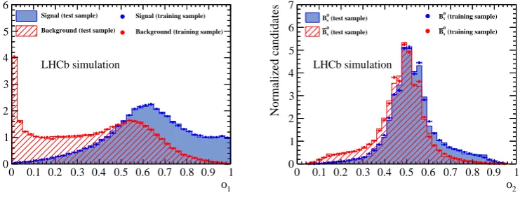
The network NN1 features one hidden layer with nine nodes. The activation function and the estimator type are chosen following the recommendations of ref. [26], to guarantee the probabilistic interpretation of the response function. The distribution of the NN1 output, o₁, for signal and background candidates is illustrated in figure 1. After requiring o₁ > 0.65, about 60% of the reconstructed B0_s → D−_sπ+ decays have at least one tagging candidate in background-subtracted data. This number corresponds to the tagging efficiency. The network configuration and theo₁ requirement are chosen to give the largest tagging power. For each tagged B0_s candidate there are on average 1.6 tagging tracks, to be combined in NN2.

2016 JINST 11 P05010

o

0 0.1 0.2 0.3 0.4 0.5 0.6 0.7 0.8 0.9 1

Normalized candidates 0 1 2 3 4 5 6

Signal (test sample) Background (test sample)

Signal (training sample) Background (training sample)

LHCb simulation

2

o

0 0.1 0.2 0.3 0.4 0.5 0.6 0.7 0.8 0.9 1

Normalized candidates 0 1 2 3 4 5 6 7 (test sample) s 0 B (test sample) s 0 B (training sample) s 0 B (training sample) s 0 B LHCb simulation

Figure 1. (Left) Distribution of the NN1 output,o₁, of signal (blue) and background (red) tracks. (Right)

Distribution of the NN2 output,o₂, of initially producedB_s0(blue) andB0_s(red) mesons. Both distributions are

obtained with simulated events. The markers represent the distributions obtained from the training samples; the solid histograms are the distributions obtained from the test samples. The good agreement between the distributions of the test and training samples shows that there is no overtraining of the classifiers.

with the greatesto₁are used. If fewer thann_maxpass, the unused input values are set to zero. The networks withn_max= 2, 3 and 4 perform very similarly and show a significantly better separation than the configurations withn_max= 1 or 5. The NN2 configuration withn_max= 3 is chosen. The main additional tagging power of this algorithm compared to the previous SSK algorithm comes from the possibility to treat events with multiple tracks of similar tagging quality, which allows a looser selection (i.e. a larger tagging efficiency) compared to the algorithm using a single tagging track. The distribution of the NN2 output,o₂, of initially producedB_s0andB0_s mesons is shown in figure1.

In the training configuration used [26], the NN2 output can be directly interpreted as the probability that aBcandidate with a given value ofo₂was initially produced as aB0_s meson,

P(B_s0|o₂) =o₂= NB0s(o2)

N_B0

s(o2)+NB0s(o2)

, (3.1)

where the second equality holds in the limit of infinite statistics, and N_B0

s(o2) and NB0s(o2) refer

to the number of initial B_s0 and B0_s mesons in the training sample with a given o₂ value. The distribution of the NN2 output of initial B_s0 mesons has a peak at o₂ values slightly larger than 0.5, while that of initialB0_s mesons has a peak ato₂values slightly smaller than 0.5 (figure1). In case of noCPasymmetries, and no asymmetries related to the different interaction probabilities of charged kaons with the detector, the NN2 distribution of initial B_s0 mesons is expected to be identical, within uncertainties, to the NN2 distribution of initial B0_s mesons mirrored ato₂ = 0.5. This is a prerequisite for interpreting the NN2 output as a mistag probability. Therefore, to ensure such an interpretation, a new variable is defined, which has a mirrored distribution for initial B0_s andB0_s mesons of the same kinematics,

o₂0 = o2+(1−o¯2)

2 , (3.2)

2016 JINST 11 P05010

aB0_sifo0₂< 0.5. Likewise, the mistag probability is defined asη =1−o0₂for candidates tagged as B0_s, and asη= o₂0 for candidates tagged asB0_s.

4 Calibration usingB0

s → D

−

sπ+ decays

The mistag probability estimated by the SSK algorithm is calibrated using two different decays, B0_s→D−_sπ+andB∗_s2(5840)0→ B+K−. The calibration withB0_s→D−_sπ+decays requires theB_s0–B0_s flavour oscillations to be resolved via a fit to theB0_s decay time distribution, since the amplitude of the oscillation is related to the mistag fraction. In contrast, there are no flavour oscillations before the strong decay of theB_s∗₂(5840)0and the charged mesons produced in its decays directly identify the

B∗_s2(5840)0production flavour. Therefore, the calibration withB_s∗₂(5840)0is performed by counting

the number of correctly and incorrectly tagged signal candidates. Thus, the two calibrations feature different analysis techniques, which are affected by different sources of systematic uncertainties, and serve as cross-checks of each other. The calibration withB_s0→ D−_sπ+decays is described in this section and that usingB_s∗₂(5840)0→B+K−decays in section5. The results are combined in section8after equalising the transverse momentum spectra of the reconstructedB_s0andB_s∗₂(5840)0

candidates, since the calibration parameters depend on the kinematics of the reconstructedBdecay. These calibrations also serve as a test of the new algorithm in data, to evaluate the performance of the tagger and to compare it to that of the previous SSK algorithm used in LHCb.

A sample of B0_s → D−_sπ+ candidates is selected according to the requirements presented in ref. [27]. TheD_s−candidates are reconstructed in the final statesK+K−π−andπ−π+π−. TheD_s−π+ mass spectrum contains a narrow peak, corresponding toB_s0→D−_sπ+signal candidates, and other broader structures due to misreconstructed b-hadron decays, all on top of a smooth background distribution due to random combinations of tracks passing the selection requirements. The signal and background components are determined by a fit to the mass distribution of candidates in the range 5100–5600 MeV/c2 (figure2). The signal component is described as the sum of two Gaussian functions with a common mean, plus a power-law tail on each side, which is fixed from simulations. The combinatorial background is modelled by an exponential function. The broad structures are due to BandΛ0_bdecays in which a final-state particle is either not reconstructed or is misidentified as a different hadron, and the mass distributions of these backgrounds are derived from simulations. The B_s0signal yield obtained from the fit is approximately 95,000. Candidates in the mass range 5320–5600 MeV/c2are selected for the calibration of the SSK algorithm. A fit to theB_s0mass distribution is performed to extractsWeights[28]; in this fit the relative fractions of the

background components are fixed by integrating the components obtained in the previous fit across the small mass window. ThesWeightsare used to subtract the background in the fit to the unbinned

distribution of the reconstructedB0_s decay time,t. This procedure for subtracting the background is validated with pseudoexperiments and provides unbiased estimates of the calibration parameters.

2016 JINST 11 P05010

]

) [MeV/c

π

m(D

5100 5200 5300 5400 5500 5600

)

2

Candidates/( 2.5 MeV/c

0 1000 2000 3000 4000 5000 6000 Data Total + π − s D → 0 s B + K − s D → 0 s B + π − s D → 0 B + π − c Λ → 0 b Λ + π − * s D → 0 s B + ρ − s D → 0 s B Combinatorial LHCb

Figure 2. Mass distribution of B_s0→ D−_sπ+ candidates with fit projections overlaid. Data points (black

markers) correspond to the B0_s candidates selected in the 3 fb−1 data sample. The total fit function and its

components are overlaid with solid and dashed lines (see legend).

is defined as unmixed if the flavours are the same. The probability density function (PDF) used to fit thetdistribution is

P(t)∝ a(t)

Γ(t0)⊗ R(t−t0), (4.1)

wheret0is the true decay time of theB0_s meson,Γ(t0)is theB_s0decay rate, R(t−t0)the decay time

resolution function, anda(t)is the decay time acceptance.

The decay rate of untagged candidates is given by

Γ(t0) ∝ (1−ε_tag)e−t0/τs cosh ∆Γs

2 t

0

!

, (4.2)

and that of tagged candidates by

Γ(t0) ∝ε_tage−t0/τs cosh ∆Γs

2 t0

!

+qmix(1−2ω) cos(∆mst0)

!

, (4.3)

whereqmixis−1 or+1 for candidates which are mixed or unmixed respectively, andωis the mistag

fraction. The average B_s0 lifetime, τs, the width difference of the Bs0 mass eigenstates, ∆Γs, and their mass difference,∆ms, are fixed to known values [2,12,29].

Each measurement oft is assumed to have a Gaussian uncertainty,σt, which is estimated by a kinematic fit of theB_s0decay chain. This uncertainty is corrected with a scale factor of 1.37, as measured with data from a sample of fake B0_s candidates, which consist of combinations of aD_s− candidate and aπ+_{candidate, both originating from a primary interaction [12]. Their decay time} distribution is aδ-function at zero convolved with the decay time resolution function,R(t−t0). The

latter is described as the sum of three Gaussian functions. The functional form ofa(t)is modelled

2016 JINST 11 P05010

η

0.1 0.15 0.2 0.25 0.3 0.35 0.4 0.45 0.5

Candidates/( 0.0025 )

0 500 1000 1500 2000

2500 LHCb

η

0 0.1 0.2 0.3 0.4 0.5

ω

0 0.1 0.2 0.3 0.4 0.5

LHCb

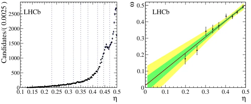
Figure 3. (Left) Background-subtractedηdistribution ofB_s0→ D−

sπ+candidates in data; the vertical dotted

lines show the binning used in the second method of the calibration. (Right) Measured average mistag

fractionωin bins of mistag probabilityη(black points), with the result of a linear fit superimposed (solid red

line) and compared to the calibration obtained from the unbinned fit (dashed black line). The linear fit has

χ2_{/ndf=1.3. The shaded areas correspond to the 68% and 95% confidence level regions of the unbinned}

fit.

Two methods are used to calibrate the mistag probability. In the first one,ηis an input variable of the fit, andωin eq. (4.3) is replaced by the calibration functionω(η), which is assumed to be a

first-order polynomial,

ω(η) =p₀+p₁(η − hηi), (4.4)

where hηi is the average of the η distribution of signal candidates (figure 3), fixed to the value

0.4377, whilep₀andp₁are the calibration parameters to be determined by the fit. They are found to be

p₀− hηi = 0.0052±0.0044(stat),

p₁ = 0.977±0.070(stat),

consistent with the expectations of a well-calibrated algorithm,p₀− hηi=0 andp₁=1. The fitted values above are considered as the nominal results of the calibration. After calibration of the mistag probability, the tagging efficiency and tagging power measured inB0_s→D−_sπ+decays are found to beε_tag= (60.38±0.16(stat))% andε_eff =(1.80±0.19(stat))%.

In the second method, the average mistag fraction ω is determined by fitting the B_s0 decay time distribution split into nine bins of mistag probability. Nine pairs (hηji, ωj) are obtained, whereωj is the mistag fraction fitted in the bin j, which has an average mistag probability hηji. The (hηji, ωj) pairs are fitted with the calibration function of eq. (4.4) to measure the calibration parametersp₀andp₁. The calibration parameters obtained,p₀− hηi=0.0050±0.0045(stat)and

p₁=0.983±0.072(stat), are in good agreement with those reported above. This method also

demonstrates the validity of the linear parametrisation (eq. (4.4)), as shown in figure3.

2016 JINST 11 P05010

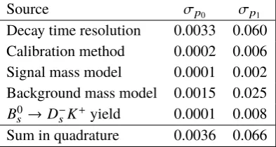
Table 1. Systematic uncertainties of the parametersp₀andp₁obtained in the calibration withB_s0→ D−_sπ+

decays.

Source σp0 σp1

Decay time resolution 0.0033 0.060 Calibration method 0.0002 0.006 Signal mass model 0.0001 0.002 Background mass model 0.0015 0.025 B0_s → D−_sK+yield 0.0001 0.008 Sum in quadrature 0.0036 0.066

The scale factor is varied by±10%, the value of its relative uncertainty, and the largest change of the

calibration parameters due to these variations is taken as the systematic uncertainty. Variations of the functions which describe the signal and the background components in the mass fit, and variations of the fraction of the main peaking background under the signal peak due toB_s0→ D−_sK+decays, result only in minor changes of the calibration parameters. The systematic uncertainties associated with these variations are assessed by generating pseudoexperiments with a range of different models and fitting them with the nominal model. Systematic uncertainties related to the parametrisation of the acceptance function, and to the parameters ∆Γ_s, τ_s and∆ms, are evaluated with the same method; no significant effect on the calibration parameters is observed. The difference between the two calibration methods reported in the previous section is assigned as a systematic uncertainty. Additionally, the calibration parameters are estimated in independent samples split according to different running periods and magnet polarities. No significant differences are observed.

5 Calibration usingB∗

s2(5840)

0 _{→ B}+_K−_decays

InB_s∗₂(5840)0→B+K− decays, theB+candidates are reconstructed in four exclusive final states, B+→ J/ψ(→ µ+µ−)K+,B+→D0(→ K+π−)π+, B+→ D0(→K+π−)π+π−π+andB+→ D0(→

K+π−π+π−)π+. The B+ candidate selection follows the same strategy as in ref. [30], retaining only those candidates with aB+mass in the range 5230–5320 MeV/c2. TheB+ candidate is then combined with a K− candidate to form a common vertex. Combinatorial background is reduced by requiring the B+ and K− candidates to have a minimum p_T of 2000 MeV/c and 250 MeV/c respectively, and to be compatible with coming from the PV. The kaon candidate must have good particle identification and a minimum momentum of 5000 MeV/c. A good-quality vertex fit of the B+K−combination is required. In order to improve the mass resolution, the invariant mass of the system,mB+K−, is computed constraining the masses of theJ/ψ (orD0) andB+candidates to their

world average values [29] and constraining the vector momenta ofB+andK−candidates to point to the associated primary vertex. Finally, theB+K−system is required to have a minimum transverse momentum of 2500 MeV/c.

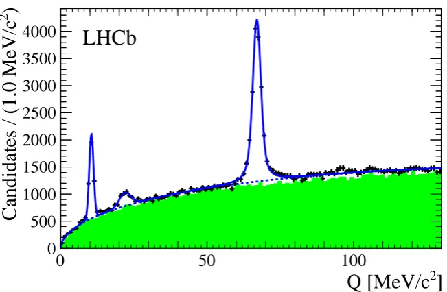
The mass difference,Q≡mB+K−−M_B+−MK−, whereM_B+andMK−are the nominal masses

2016 JINST 11 P05010

]

Q [MeV/c

0

50

100

)

2

Candidates / (1.0 MeV/c

0

500

1000

1500

2000

2500

3000

3500

4000

_LHCb

Figure 4. Distribution of the mass difference,Q, of selectedB+K−candidates, summing over fourB+decay

modes (black points), and the function fitted to these data (solid blue line). From left to right, the three peaks are identified as being Bs1(5830)0 → B∗+K−, B∗_s2(5840)0 → B∗+K−, and B_s∗₂(5840)0→B+K−. Same

charge combinationsB±K±in data are superimposed (solid histogram) and contain no structure.

asBs1(5830)0→B∗+(→B+γ)K−, B∗_s2(5840)0→B∗+(→B+γ)K−andB_s∗₂(5840)0→B+K−, re-spectively. The first two peaks are shifted down byM_B∗+−M_B+ =45.0±0.4 MeV/c2from to their nominalQ-values due to the unreconstructed photons in theB∗+decays.

The yields of the three peaks are obtained through a fit of the Q distribution in the range shown. Both the Bs1(5830)0 → B∗+K−and the B_s∗₂(5840)0 → B∗+K− signals are described by Gaussian functions. TheB∗_s2(5840)0→B+K−signal is parametrised as a relativistic Breit-Wigner function convolved with a Gaussian function to account for the detector resolution. This resolution is fixed to the value determined in the simulation (' 1 MeV/c2). The background is modelled by the function f(Q) =QαeβQ, whereαand βare free parameters. The yields of the three peaks are found to be approximately 2,900, 1,200 and 12,700, respectively. The mass and width parameters are in agreement with those obtained in ref. [30]. Only the third peak, corresponding to the fully reconstructedB_s∗₂(5840)0meson, is used in the calibration of the mistag probability.

Since the B_s∗₂(5840)0 meson is flavour-tagged by the charges of the final-state particles of

its decay, the mistag fraction can be determined by comparing the tagging decision of the SSK algorithm with the known B∗_s2(5840)0 flavour. From the fit of the Q distribution, sWeights are

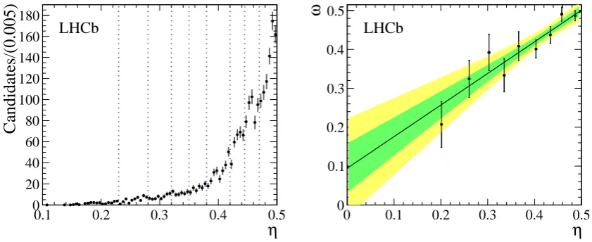
obtained and used to statistically disentangle the signal from the combinatorial background. The fit is performed separately on theQdistributions of correctly and incorrectly tagged candidates, to allow for different background fractions in the two categories. In these fits the mass parameters are fixed to the values obtained in the fit to all candidates. In figure5theη distribution of signal candidates and the mistag fractionωin bins ofηare shown. Each bin ofηhas an average predicted mistaghηi. The(hηi, ω)pairs are fitted with the calibration function of eq. (4.4) to determine the

2016 JINST 11 P05010

η

0.1 0.2 0.3 0.4 0.5

Candidates/(0.005)

0 20 40 60 80 100 120 140 160 180

LHCb

η

0 0.1 0.2 0.3 0.4 0.5

ω

0 0.1 0.2 0.3 0.4 0.5

LHCb

Figure 5. (Left) Background-subtracted η distribution of B∗

s2(5840)0→B+K

− _{candidates in data; the}

vertical dotted lines show the binning used in the calibration. (Right) Measured average mistag fractionωin

bins of mistag probabilityη(black points), with the result of a linear fit superimposed (solid black line). The

fit has χ2_{/ndf=0.8. The shaded areas correspond to the 68% and 95% confidence level regions of the fit.}

The calibration parameters depend on the kinematics of the reconstructed B meson, and in particular on its transverse momentum. In order to test whether the calibrations are consistent between the two samples, theB∗_s2(5840)0 p_Tspectrum must be reweighted to match that of theB0_s candidates seen inB0_s→D−_sπ+decays. This is done for each of the fourB+decay modes separately. Due to the requirement of a higher minimump_Tof theB∗_s2(5840)0candidates, 2.5 GeV/c, compared to 2.0 GeV/cfor the B0_s candidates, a 1% difference in the mean value of the p_T spectra remains. This is covered by the systematic uncertainties discussed in section6, which account for differences in the mean transverse momenta of Bmesons of up to 30%. The calibration parameters obtained from the full sample of weightedB_s∗₂(5840)0decays are

p₀− hηi = 0.012±0.008(stat),

p₁ = 0.813±0.123(stat),

wherehηiis fixed to the value 0.441. They are consistent within statistical uncertainties with the

calibration parameters obtained withB_s0→ D−_sπ+decays.

The systematic uncertainties of the calibration parameters are determined by repeating the calibration under different conditions. In each case the fit to theQdistribution is repeated and the

sWeightsare calculated. A summary of all of the systematic uncertainties is given in table2. To

test for potential differences in the signal model for correctly and incorrectly tagged candidates, the fit to theQ distribution is repeated for both subsets of B_s∗₂(5840)0 candidates without fixing the

mass parameters to the values obtained in the fit to all candidates. The background fit model is tested by fitting theQdistribution of correctly and incorrectly tagged candidates with the default background model replaced by a second-order polynomial, and with the fit range limited to 40 < Q<100 MeV/c2. The mass resolution forB_s∗₂(5840)0is varied by±10% to account for differences

in resolution between data and simulation. Potential biases due to theB_s∗₂(5840)0signal selection

2016 JINST 11 P05010

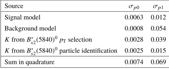
Table 2. Systematic uncertainties of the parametersp₀andp₁obtained in the calibration withB∗_s2(5840)0→

B+K−decays.

Source σp0 σp1

Signal model 0.0063 0.012

Background model 0.0008 0.054

KfromB_s∗₂(5840)0p_T selection 0.0028 0.039

KfromB_s∗₂(5840)0particle identification 0.0025 0.015

Sum in quadrature 0.0074 0.069

the kaon produced in the B∗_s2(5840)0 decay and repeating the full calibration procedure. To test

the background subtraction procedure, an alternative method of performing the calibration is used. The sample of tagged candidates is divided into bins ofη, and, in each bin, theQdistributions of correctly and incorrectly tagged candidates are fitted separately. The measured signal yields of the B∗_s2(5840)0peak are used to calculate the mistag fractionωwhich is plotted against the averageη

of each bin. The calibration parameters obtained are in agreement within statistical uncertainties with those determined from the default method.

The variation of the calibration parameters with data-taking conditions is checked by repeating the calibration procedure after splitting the candidate sample according to the data-taking period and magnet polarity. No significant variation is observed. The calibration is also repeated separately on each of the fourB+decay modes, after weighting the transverse momentum spectra. The parameters obtained agree within statistical uncertainties.

6 Portability to different decay channels

2016 JINST 11 P05010

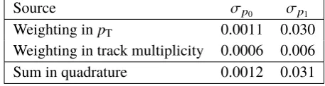
Table 3. Systematic uncertainties of the parametersp₀andp₁related to the portability of the calibration to

different decay modes.

Source σp₀ σp₁

Weighting inp_T 0.0011 0.030

Weighting in track multiplicity 0.0006 0.006

Sum in quadrature 0.0012 0.031

7 Flavour-tagging asymmetry

The calibration parameters depend on the initial flavour of the B_s0 meson, due to the different interaction cross-sections ofK+andK−with matter. Therefore, additional calibration parameters,

∆p₀ and∆p₁, are introduced to take this flavour dependence into account. The mistag fraction of mesons produced with initial flavourB0_s (accompanied by aK+) and mesons produced with initial flavourB0_s(accompanied by aK−) are given by

ω(η) = p₀+ ∆p0

2 + p1+ ∆p₁

2

!

(η − hηi)and (7.1)

ω(η) = p₀− ∆p0

2 + p1− ∆p₁

2

!

(η − hηi), (7.2)

respectively. The statistical power of the B0_s → D−_sπ+ data sample is not sufficient to determine these additional parameters, so they are studied withD−_s →φ(→K+K−)π−decays. TheD_s−mesons produced in the primary interaction are also accompanied by charged kaons produced in thecquark hadronisation. The SSK algorithm can tag the initial flavour of theD_s−candidate, with a tagging decision opposite to the case ofB0_s mesons. TheD−_s meson is charged and does not oscillate, so its initial flavour can be determined from the charge of the decay products. This can then be compared to the SSK tagging decision, and a calibration can be performed with the same method used with B∗_s2(5840)0→B+K−decays. The∆p₀and∆p₁parameters can be determined by the difference in the calibration parameters obtained withD−_s andD+_s decays.

A high-purity sample ofD−_s →φ(→K+K−)π−candidates is selected in a sample

correspond-ing to 3 fb−1 _{of data taken at centre-of-mass energies of 7 and 8 TeV by applying the following}

criteria. The momenta of the final-state particles must be larger than 2 GeV/cand their transverse momenta larger than 250 MeV/c. The tracks must be significantly displaced from the primary vertex. Their associated particle type information is required to be consistent with a kaon or a pion, as appropriate. The K+K− invariant mass must be within 7 MeV/c2 of the known φmass. The φ and the D−_s reconstructed vertices must be of good quality. The momentum vector of the D_s− candidate must be consistent with the displacement vector between the primary vertex and theD_s− decay vertex. Only candidates with a reconstructedD−_s mass in the range 1920–2040 MeV/c2 are considered. The resultingD_s−mass distribution is fitted by a sum of two Gaussian functions with a common mean to describe the signal component, and an exponential function for the combinatorial background (figure6). In total about 784,000 signal candidates are reconstructed with a background fraction below 5%. From the mass fit,sWeightsare calculated to subtract the background in theη

2016 JINST 11 P05010

]

2

) [MeV/c −

π − K

+

m(K

1950 2000

)

2

Candidates/( 1.2 MeV/c

0 20 40 60

3

10

×

/dof = 2.94 2

χ

LHCb Preliminary Data 2011+2012 LHCb

Data

Total

− π −

K

+

K

→ − s

D

Combinatorial

Figure 6. Mass distribution ofD−_s →φ(→K+K−)π−candidates with fit projections overlaid. Data points

(black markers) correspond to theD−_s candidates selected in the 3 fb−1data sample. The total fit function

and its components are overlaid (see legend).

the B_s0 kinematics are accounted for by weighting the D_s−candidates to match the B_s0 transverse momentum distribution measured with B0_s → D−_sπ+ decays. The average mistag probability in eq. (7.3) is fixed to the value found forB_s0→D−_sπ+decays, 0.4377. The parameters related to the flavour-tagging asymmetries are found to be

∆p₀ = −0.0163±0.0022(stat)±0.0030(syst),

∆p₁ = −0.031±0.025(stat)±0.045(syst),

∆ε_tag = (0.17±0.11(stat)±0.68(syst))%, (7.3)

where∆ε_tag≡ε_tag(D−_s)−ε_tag(D_s+) =ε_tag(B0_s)−ε_tag(B0_s).

A systematic uncertainty is computed by taking the maximum of the differences seen when comparing these calibration parameters and those obtained by weighting the transverse momentum distribution of theD_s−candidates to match the followingB_s0decay modes: B_s0→ J/ψ φ, B0_s →φφ

B0_s →D+_sD_s−. These uncertainties are 0.0030 and 0.040 for∆p₀ and∆p₁respectively, and 0.66% for ∆ε_tag. The same procedure is applied to assess the systematic uncertainty associated with the different track multiplicity distribution betweenD_s+andB0_s decays (0.0002 and 0.020 for∆p₀ and∆p₁respectively, and 0.15% for∆ε_tag). The systematic uncertainty in eq. (7.3) is the sum in quadrature of these two sources of uncertainties.

While the shift of the slope parameter∆p₁is compatible with zero, there is a significant overall shift, ∆p₀, of about 1.6% towards higher mistag rates for B0_s particles. This can be explained by the higher interaction rate in matter of K− particles compared toK+ particles. These values are consistent with results obtained in simulated samples ofB0_s→D−_sπ+andB0_s→ J/ψ φdecays.

The B∗_s2(5840)0 decays can also be used to measure the values of∆p₀, ∆p₁ and∆ε_tag. The

2016 JINST 11 P05010

measured in the promptD−_s meson sample.

8 Calibration summary

The final calibration parameters are computed as the weighted average of the results obtained in B0_s→ D−_sπ+andB_s∗₂(5840)0→B+K−decays, fixinghηi=0.4377 and considering the systematic

uncertainties reported in tables 1 and 2 to be uncorrelated. The uncertainties relating to the portability of the calibrations to different B0_s decays as reported in table 3 are considered to be fully correlated. For the flavour-tagging asymmetries, only the results measured in D−_s decays are considered. The final values are

hηi = 0.4377,

p₀− hηi = 0.0070±0.0039(stat)±0.0035(syst),

p₁ = 0.925±0.061(stat)±0.059(syst),

∆p₀ = −0.0163±0.0022(stat)±0.0030(syst),

∆p₁ = −0.031±0.025(stat)±0.045(syst),

∆ε_tag = (0.17±0.11(stat)±0.68(syst))%.

9 Possible application to OS kaons

The two-step neural-network approach of the SSK tagging algorithm presented here is a promising method for improving any tagging algorithm which needs to combine information from multiple tagging tracks. A natural candidate for the application of this method is the OS kaon tagging algorithm, which searches for kaons fromb→c →stransitions of the OSbhadron. The current implementation of the OS kaon algorithm selects tracks with large impact parameters with respect to the primary vertex associated with the signalBmeson [6]. This selection gives a tagging efficiency of about 15%. A preliminary implementation of a neural-network-based algorithm shows that loosening the impact parameter requirements for the track candidates and using the new approach increases the tagging efficiency to about 70% and significantly improves the effective tagging efficiency ofB+andB0 mesons. However, the inclusion of kaons with smaller impact parameters results in up to 10% of the signal fragmentation tracks being assigned as OS kaon candidates. As the correlation of signal fragmentation kaons with the signal Bflavour is different for B+, B0 and B_s0 mesons, this contamination of SS kaon tracks introduces a dependence of the calibration parameters on theBmeson species, and the gain in tagging performance observed inB+andB0is not reproduced inB_s0mesons.

10 Conclusion

2016 JINST 11 P05010

with data corresponding to an integrated luminosity of 3 fb−1_{collected by the LHCb experiment in}

proton-proton collisions at 7 and 8 TeV centre-of-mass energies. The calibration is performed in two ways: by resolving theB_s0–B0_sflavour oscillations inB0_s→D−_sπ+decays, and, for the first time, by analysing flavour-specificB∗_s2(5840)0→B+K−strong decays.

The tagging power of the new algorithm as measured in B0_s → D−_sπ+ decays is (1.80±

0.19(stat) ±0.18(syst))%, a significant improvement over the tagging power of 1.2% of the

previous implementation used at the LHCb experiment. This new algorithm represents important progress for many analyses aiming to make high-precision measurements ofB_s0–B0_s mixing andCP asymmetries ofB_s0decays. Its performance has been demonstrated in several recent measurements by the LHCb collaboration [2,3,27,31,32].

Acknowledgments

We express our gratitude to our colleagues in the CERN accelerator departments for the excellent performance of the LHC. We thank the technical and administrative staff at the LHCb institutes. We acknowledge support from CERN and from the national agencies: CAPES, CNPq, FAPERJ and FINEP (Brazil); NSFC (China); CNRS/IN2P3 (France); BMBF, DFG and MPG (Germany); INFN (Italy); FOM and NWO (The Netherlands); MNiSW and NCN (Poland); MEN/IFA (Romania); MinES and FANO (Russia); MinECo (Spain); SNSF and SER (Switzerland); NASU (Ukraine); STFC (United Kingdom); NSF (U.S.A.). We acknowledge the computing resources that are provided by CERN, IN2P3 (France), KIT and DESY (Germany), INFN (Italy), SURF (The Netherlands), PIC (Spain), GridPP (United Kingdom), RRCKI and Yandex LLC (Russia), CSCS (Switzerland), IFIN-HH (Romania), CBPF (Brazil), PL-GRID (Poland) and OSC (U.S.A.). We are indebted to the communities behind the multiple open source software packages on which we depend. Individual groups or members have received support from AvH Foundation (Germany), EPLANET, Marie Skłodowska-Curie Actions and ERC (European Union), Conseil Général de Haute-Savoie, Labex ENIGMASS and OCEVU, Région Auvergne (France), RFBR and Yandex LLC (Russia), GVA, XuntaGal and GENCAT (Spain), Herchel Smith Fund, The Royal Society, Royal Commission for the Exhibition of 1851 and the Leverhulme Trust (United Kingdom).

References

[1] LHCb collaboration,Implications of LHCb measurements and future prospects,Eur. Phys. J.C 73

(2013) 2373[arXiv:1208.3355].

[2] LHCb collaboration,Precision measurement ofCPviolation inB0_s→ J/ψK+K−decays,Phys. Rev.

Lett.114(2015) 041801[arXiv:1411.3104].

[3] LHCb collaboration,Measurement of theCP-violating phaseφsinB

0

s→ J/ψπ+π−decays,Phys.

Lett.B 736(2014) 186[arXiv:1405.4140].

[4] LHCb collaboration,Roadmap for selected key measurements of LHCb,arXiv:0912.4179.

[5] LHCb collaboration,Letter of intent for the LHCb upgrade,CERN-LHCC-2011-001(2011).

[6] LHCb collaboration,Opposite-side flavour tagging of B mesons at the LHCb experiment,Eur. Phys.

2016 JINST 11 P05010

[7] LHCb collaboration,Bflavour tagging using charm decays at the LHCb experiment,2015JINST10

P10005[arXiv:1507.07892].

[8] M. Gronau, A. Nippe and J.L. Rosner,Method for flavor tagging in neutral B meson decays,Phys.

Rev.D 47(1993) 1988[hep-ph/9211311].

[9] CDF collaboration, F. Abe et al.,Measurement of theB0–B0flavor oscillation frequency and study of

same side flavor tagging ofBmesons inpp¯collisions,Phys. Rev.D 59(1999) 032001

[hep-ex/9806026].

[10] CDF collaboration, A. Abulencia et al.,Measurement of theB0_s–B0_sOscillation Frequency,Phys. Rev.

Lett.97(2006) 062003[hep-ex/0606027].

[11] LHCb collaboration,Measurement ofCP-violation and theB0_smeson decay width difference with

B_s0→ J/ψK+K−_andB0

s → J/ψπ+π−decays,Phys. Rev.D 87(2013) 112010[arXiv:1304.2600].

[12] LHCb collaboration,Precision measurement of theB_s0–B0_soscillation frequency with the decay

B_s0→D_s−π+,New J. Phys.15(2013) 053021[arXiv:1304.4741].

[13] LHCb collaboration,The LHCb Detector at the LHC,2008JINST3S08005.

[14] LHCb collaboration,LHCb Detector Performance,Int. J. Mod. Phys.A 30(2015) 1530022

[arXiv:1412.6352].

[15] R. Aaij et al.,The LHCb Trigger and its Performance in 2011,2013JINST 8P04022

[arXiv:1211.3055].

[16] V.V. Gligorov and M. Williams,Efficient, reliable and fast high-level triggering using a bonsai

boosted decision tree,2013JINST8P02013[arXiv:1210.6861].

[17] T. Sjöstrand, S. Mrenna and P.Z. Skands,PYTHIA 6.4 Physics and Manual,JHEP05(2006) 026

[hep-ph/0603175].

[18] T. Sjöstrand, S. Mrenna and P.Z. Skands,A Brief Introduction to PYTHIA 8.1,Comput. Phys.

Commun.178(2008) 852[arXiv:0710.3820].

[19] LHCb collaboration,Handling of the generation of primary events in Gauss, the LHCb simulation

framework,J. Phys. Conf. Ser.331(2011) 032047.

[20] D.J. Lange,The EvtGen particle decay simulation package,Nucl. Instrum. Meth.A 462(2001) 152.

[21] P. Golonka and Z. Was,PHOTOS Monte Carlo: A Precision tool for QED corrections inZandW

decays,Eur. Phys. J.C 45(2006) 97[hep-ph/0506026].

[22] Geant4 collaboration, J. Allison et al.,Geant4 developments and applications,IEEE Trans. Nucl.

Sci.53(2006) 270.

[23] GEANT4 collaboration, S. Agostinelli et al.,GEANT4: A Simulation toolkit,Nucl. Instrum. Meth.A

506(2003) 250.

[24] LHCb collaboration, M. Clemencic et al.,The LHCb simulation application, Gauss: Design,

evolution and experience,J. Phys. Conf. Ser.331(2011) 032023.

[25] J.-H. Zhong, R.-S. Huang, S.-C. Lee, R.-S. Huang and S.-C. Lee,A program for the Bayesian Neural

Network in the ROOT framework,Comput. Phys. Commun.182(2011) 2655[arXiv:1103.2854].

[26] L. Breiman, J.H. Friedman, R.A. Olshen and C.J. Stone,Classification and regression trees,

Wadsworth international group, Belmont California U.S.A. (1984).

[27] LHCb collaboration,Measurement ofCPasymmetry inB_s0→ D∓_sK±decays,JHEP11(2014) 060

2016 JINST 11 P05010

[28] M. Pivk and F.R. Le Diberder,sPlot: A Statistical tool to unfold data distributions,Nucl. Instrum.

Meth.A 555(2005) 356[physics/0402083].

[29] Particle Data Group collaboration, K.A. Olive et al.,Review of Particle Physics,Chin. Phys.C 38

(2014) 090001and 2015 update.

[30] LHCb collaboration,First observation of the decayB∗_s2(5840)0→B∗+K−and studies of excitedB_s0 mesons,Phys. Rev. Lett.110(2013) 151803[arXiv:1211.5994].

[31] LHCb collaboration,Measurement ofCP-violation inB0_s →φφdecays,Phys. Rev.D 90(2014)

052011[arXiv:1407.2222].

[32] LHCb collaboration,Measurement of theCP-violating phaseφsinB

0

s→D+sD−s decays,Phys. Rev.

2016 JINST 11 P05010

R. Aaij39_{, C. Abellán Beteta}41_{, B. Adeva}38_{, M. Adinolfi}47_{, A. Affolder}53_{, Z. Ajaltouni}5_{, S. Akar}6_,

J. Albrecht10_{, F. Alessio}39_{, M. Alexander}52_{, S. Ali}42_{, G. Alkhazov}31_{, P. Alvarez Cartelle}54_{, A.A. Alves Jr}58_,

S. Amato2_{, S. Amerio}23_{, Y. Amhis}7_{, L. An}3,40_{, L. Anderlini}18_{, G. Andreassi}40_{, M. Andreotti}17,g_,

J.E. Andrews59_{, R.B. Appleby}55_{, O. Aquines Gutierrez}11_{, F. Archilli}39_{, P. d’Argent}12_{, A. Artamonov}36_,

M. Artuso60_{, E. Aslanides}6_{, G. Auriemma}26,n_{, M. Baalouch}5_{, S. Bachmann}12_{, J.J. Back}49_{, A. Badalov}37_,

C. Baesso61_{, W. Baldini}17,39_{, R.J. Barlow}55_{, C. Barschel}39_{, S. Barsuk}7_{, W. Barter}39_{, V. Batozskaya}29_,

V. Battista40_{, A. Bay}40_{, L. Beaucourt}4_{, J. Beddow}52_{, F. Bedeschi}24_{, I. Bediaga}1_{, L.J. Bel}42_{, V. Bellee}40_,

N. Belloli21,k_{, I. Belyaev}32_{, E. Ben-Haim}8_{, G. Bencivenni}19_{, S. Benson}39_{, J. Benton}47_{, A. Berezhnoy}33_,

R. Bernet41_{, A. Bertolin}23_{, F. Betti}15_{, M.-O. Bettler}39_{, M. van Beuzekom}42_{, S. Bifani}46_{, P. Billoir}8_,

T. Bird55_{, A. Birnkraut}10_{, A. Bizzeti}18,i_{, T. Blake}49_{, F. Blanc}40_{, J. Blouw}11_{, S. Blusk}60_{, V. Bocci}26_,

A. Bondar35_{, N. Bondar}31,39_{, W. Bonivento}16_{, A. Borgheresi}21,k_{, S. Borghi}55_{, M. Borisyak}66_{, M. Borsato}38_,

T.J.V. Bowcock53_{, E. Bowen}41_{, C. Bozzi}17,39_{, S. Braun}12_{, M. Britsch}12_{, T. Britton}60_{, J. Brodzicka}55_,

N.H. Brook47_{, E. Buchanan}47_{, C. Burr}55_{, A. Bursche}41_{, J. Buytaert}39_{, S. Cadeddu}16_{, R. Calabrese}17,g_,

M. Calvi21,k_{, M. Calvo Gomez}37,p_{, P. Campana}19_{, D. Campora Perez}39_{, L. Capriotti}55_{, A. Carbone}15,e_,

G. Carboni25,l_{, R. Cardinale}20,j_{, A. Cardini}16_{, P. Carniti}21,k_{, L. Carson}51_{, K. Carvalho Akiba}2_{, G. Casse}53_,

L. Cassina21,k_{, L. Castillo Garcia}40_{, M. Cattaneo}39_{, Ch. Cauet}10_{, G. Cavallero}20_{, R. Cenci}24,t_{, M. Charles}8_,

Ph. Charpentier39_{, G. Chatzikonstantinidis}46_{, M. Chefdeville}4_{, S. Chen}55_{, S.-F. Cheung}56_{, N. Chiapolini}41_,

M. Chrzaszcz41,27_{, X. Cid Vidal}39_{, G. Ciezarek}42_{, P.E.L. Clarke}51_{, M. Clemencic}39_{, H.V. Cliff}48_,

J. Closier39_{, V. Coco}39_{, J. Cogan}6_{, E. Cogneras}5_{, V. Cogoni}16,f_{, L. Cojocariu}30_{, G. Collazuol}23,r_,

P. Collins39_{, A. Comerma-Montells}12_{, A. Contu}39_{, A. Cook}47_{, M. Coombes}47_{, S. Coquereau}8_{, G. Corti}39_,

M. Corvo17,g_{, B. Couturier}39_{, G.A. Cowan}51_{, D.C. Craik}51_{, A. Crocombe}49_{, M. Cruz Torres}61_,

S. Cunliffe54_{, R. Currie}54_{, C. D’Ambrosio}39_{, E. Dall’Occo}42_{, J. Dalseno}47_{, P.N.Y. David}42_{, A. Davis}58_,

O. De Aguiar Francisco2_{, K. De Bruyn}6_{, S. De Capua}55_{, M. De Cian}12_{, J.M. De Miranda}1_{, L. De Paula}2_,

P. De Simone19_{, C.-T. Dean}52_{, D. Decamp}4_{, M. Deckenhoff}10_{, L. Del Buono}8_{, N. Déléage}4_{, M. Demmer}10_,

D. Derkach66_{, O. Deschamps}5_{, F. Dettori}39_{, B. Dey}22_{, A. Di Canto}39_{, F. Di Ruscio}25_{, H. Dijkstra}39_,

S. Donleavy53_{, F. Dordei}39_{, M. Dorigo}40_{, A. Dosil Suárez}38_{, A. Dovbnya}44_{, K. Dreimanis}53_{, L. Dufour}42_,

G. Dujany55_{, K. Dungs}39_{, P. Durante}39_{, R. Dzhelyadin}36_{, A. Dziurda}27_{, A. Dzyuba}31_{, S. Easo}50,39_,

U. Egede54_{, V. Egorychev}32_{, S. Eidelman}35_{, S. Eisenhardt}51_{, U. Eitschberger}10_{, R. Ekelhof}10_{, L. Eklund}52_,

I. El Rifai5_{, Ch. Elsasser}41_{, S. Ely}60_{, S. Esen}12_{, H.M. Evans}48_{, T. Evans}56_{, A. Falabella}15_{, C. Färber}39_,

N. Farley46_{, S. Farry}53_{, R. Fay}53_{, D. Fazzini}21,k_{, D. Ferguson}51_{, V. Fernandez Albor}38_{, F. Ferrari}15_,

F. Ferreira Rodrigues1_{, M. Ferro-Luzzi}39_{, S. Filippov}34_{, M. Fiore}17,39,g_{, M. Fiorini}17,g_{, M. Firlej}28_,

C. Fitzpatrick40_{, T. Fiutowski}28_{, F. Fleuret}7,b_{, K. Fohl}39_{, P. Fol}54_{, M. Fontana}16_{, F. Fontanelli}20,j_{, D.}

C. Forshaw60_{, R. Forty}39_{, M. Frank}39_{, C. Frei}39_{, M. Frosini}18_{, J. Fu}22_{, E. Furfaro}25,l_{, A. Gallas Torreira}38_,

D. Galli15,e_{, S. Gallorini}23_{, S. Gambetta}51_{, M. Gandelman}2_{, P. Gandini}56_{, Y. Gao}3_{, J. García Pardiñas}38_,

J. Garra Tico48_{, L. Garrido}37_{, D. Gascon}37_{, C. Gaspar}39_{, L. Gavardi}10_{, G. Gazzoni}5_{, D. Gerick}12_,

E. Gersabeck12_{, M. Gersabeck}55_{, T. Gershon}49_{, Ph. Ghez}4_{, S. Gianì}40_{, V. Gibson}48_{, O.G. Girard}40_,

L. Giubega30_{, V.V. Gligorov}39_{, C. Göbel}61_{, D. Golubkov}32_{, A. Golutvin}54,39_{, A. Gomes}1,a_{, C. Gotti}21,k_,

M. Grabalosa Gándara5_{, R. Graciani Diaz}37_{, L.A. Granado Cardoso}39_{, E. Graugés}37_{, E. Graverini}41_,

G. Graziani18_{, A. Grecu}30_{, P. Griffith}46_{, L. Grillo}12_{, O. Grünberg}64_{, B. Gui}60_{, E. Gushchin}34_{, Yu. Guz}36,39_,

T. Gys39_{, T. Hadavizadeh}56_{, C. Hadjivasiliou}60_{, G. Haefeli}40_{, C. Haen}39_{, S.C. Haines}48_{, S. Hall}54_,

B. Hamilton59_{, X. Han}12_{, S. Hansmann-Menzemer}12_{, N. Harnew}56_{, S.T. Harnew}47_{, J. Harrison}55_{, J. He}39_,

T. Head40_{, V. Heijne}42_{, A. Heister}9_{, K. Hennessy}53_{, P. Henrard}5_{, L. Henry}8_{, J.A. Hernando Morata}38_,

E. van Herwijnen39_{, M. Heß}64_{, A. Hicheur}2_{, D. Hill}56_{, M. Hoballah}5_{, C. Hombach}55_{, W. Hulsbergen}42_,

T. Humair54_{, M. Hushchyn}66_{, N. Hussain}56_{, D. Hutchcroft}53_{, D. Hynds}52_{, M. Idzik}28_{, P. Ilten}57_,

R. Jacobsson39_{, A. Jaeger}12_{, J. Jalocha}56_{, E. Jans}42_{, A. Jawahery}59_{, M. John}56_{, D. Johnson}39_{, C.R. Jones}48_,

C. Joram39_{, B. Jost}39_{, N. Jurik}60_{, S. Kandybei}44_{, W. Kanso}6_{, M. Karacson}39_{, T.M. Karbach}39,†_,

2016 JINST 11 P05010

B. Khanji21,39,k_{, C. Khurewathanakul}40_{, T. Kirn}9_{, S. Klaver}55_{, K. Klimaszewski}29_{, O. Kochebina}7_,

M. Kolpin12_{, I. Komarov}40_{, R.F. Koopman}43_{, P. Koppenburg}42,39_{, M. Kozeiha}5_{, L. Kravchuk}34_,

K. Kreplin12_{, M. Kreps}49_{, G. Krocker}12_{, P. Krokovny}35_{, F. Kruse}10_{, W. Krzemien}29_{, W. Kucewicz}27,o_,

M. Kucharczyk27_{, V. Kudryavtsev}35_{, A. K. Kuonen}40_{, K. Kurek}29_{, T. Kvaratskheliya}32_{, D. Lacarrere}39_,

G. Lafferty55,39_{, A. Lai}16_{, D. Lambert}51_{, G. Lanfranchi}19_{, C. Langenbruch}49_{, B. Langhans}39_{, T. Latham}49_,

C. Lazzeroni46_{, R. Le Gac}6_{, J. van Leerdam}42_{, J.-P. Lees}4_{, R. Lefèvre}5_{, A. Leflat}33,39_{, J. Lefrançois}7_,

E. Lemos Cid38_{, O. Leroy}6_{, T. Lesiak}27_{, B. Leverington}12_{, Y. Li}7_{, T. Likhomanenko}66,65_{, M. Liles}53_,

R. Lindner39_{, C. Linn}39_{, F. Lionetto}41_{, B. Liu}16_{, X. Liu}3_{, D. Loh}49_{, I. Longstaff}52_{, J.H. Lopes}2_,

D. Lucchesi23,r_{, M. Lucio Martinez}38_{, H. Luo}51_{, A. Lupato}23_{, E. Luppi}17,g_{, O. Lupton}56_{, N. Lusardi}22_,

A. Lusiani24_{, F. Machefert}7_{, F. Maciuc}30_{, O. Maev}31_{, K. Maguire}55_{, S. Malde}56_{, A. Malinin}65_{, G. Manca}7_,

G. Mancinelli6_{, P. Manning}60_{, A. Mapelli}39_{, J. Maratas}5_{, J.F. Marchand}4_{, U. Marconi}15_{, C. Marin Benito}37_,

P. Marino24,39,t_{, J. Marks}12_{, G. Martellotti}26_{, M. Martin}6_{, M. Martinelli}40_{, D. Martinez Santos}38_,

F. Martinez Vidal67_{, D. Martins Tostes}2_{, L.M. Massacrier}7_{, A. Massafferri}1_{, R. Matev}39_{, A. Mathad}49_,

Z. Mathe39_{, C. Matteuzzi}21_{, A. Mauri}41_{, B. Maurin}40_{, A. Mazurov}46_{, M. McCann}54_{, J. McCarthy}46_,

A. McNab55_{, R. McNulty}13_{, B. Meadows}58_{, F. Meier}10_{, M. Meissner}12_{, D. Melnychuk}29_{, M. Merk}42_,

A Merli22,u_{, E Michielin}23_{, D.A. Milanes}63_{, M.-N. Minard}4_{, D.S. Mitzel}12_{, J. Molina Rodriguez}61_,

I.A. Monroy63_{, S. Monteil}5_{, M. Morandin}23_{, P. Morawski}28_{, A. Mordà}6_{, M.J. Morello}24,t_{, J. Moron}28_,

A.B. Morris51_{, R. Mountain}60_{, F. Muheim}51_{, D. Müller}55_{, J. Müller}10_{, K. Müller}41_{, V. Müller}10_,

M. Mussini15_{, B. Muster}40_{, P. Naik}47_{, T. Nakada}40_{, R. Nandakumar}50_{, A. Nandi}56_{, I. Nasteva}2_,

M. Needham51_{, N. Neri}22_{, S. Neubert}12_{, N. Neufeld}39_{, M. Neuner}12_{, A.D. Nguyen}40_{, C. Nguyen-Mau}40,q_,

V. Niess5_{, S. Nieswand}9_{, R. Niet}10_{, N. Nikitin}33_{, T. Nikodem}12_{, A. Novoselov}36_{, D.P. O’Hanlon}49_,

A. Oblakowska-Mucha28_{, V. Obraztsov}36_{, S. Ogilvy}52_{, O. Okhrimenko}45_{, R. Oldeman}16,48,f_,

C.J.G. Onderwater68_{, B. Osorio Rodrigues}1_{, J.M. Otalora Goicochea}2_{, A. Otto}39_{, P. Owen}54_,

A. Oyanguren67_{, A. Palano}14,d_{, F. Palombo}22,u_{, M. Palutan}19_{, J. Panman}39_{, A. Papanestis}50_,

M. Pappagallo52_{, L.L. Pappalardo}17,g_{, C. Pappenheimer}58_{, W. Parker}59_{, C. Parkes}55_{, G. Passaleva}18_,

G.D. Patel53_{, M. Patel}54_{, C. Patrignani}20,j_{, A. Pearce}55,50_{, A. Pellegrino}42_{, G. Penso}26,m_,

M. Pepe Altarelli39_{, S. Perazzini}15,e_{, P. Perret}5_{, L. Pescatore}46_{, K. Petridis}47_{, A. Petrolini}20,j_{, M. Petruzzo}22_,

E. Picatoste Olloqui37_{, B. Pietrzyk}4_{, M. Pikies}27_{, D. Pinci}26_{, A. Pistone}20_{, A. Piucci}12_{, S. Playfer}51_,

M. Plo Casasus38_{, T. Poikela}39_{, F. Polci}8_{, A. Poluektov}49,35_{, I. Polyakov}32_{, E. Polycarpo}2_{, A. Popov}36_,

D. Popov11,39_{, B. Popovici}30_{, C. Potterat}2_{, E. Price}47_{, J.D. Price}53_{, J. Prisciandaro}38_{, A. Pritchard}53_,

C. Prouve47_{, V. Pugatch}45_{, A. Puig Navarro}40_{, G. Punzi}24,s_{, W. Qian}56_{, R. Quagliani}7,47_{, B. Rachwal}27_,

J.H. Rademacker47_{, M. Rama}24_{, M. Ramos Pernas}38_{, M.S. Rangel}2_{, I. Raniuk}44_{, G. Raven}43_{, F. Redi}54_,

S. Reichert55_{, A.C. dos Reis}1_{, V. Renaudin}7_{, S. Ricciardi}50_{, S. Richards}47_{, M. Rihl}39_{, K. Rinnert}53,39_,

V. Rives Molina37_{, P. Robbe}7,39_{, A.B. Rodrigues}1_{, E. Rodrigues}55_{, J.A. Rodriguez Lopez}63_,

P. Rodriguez Perez55_{, A. Rogozhnikov}66_{, S. Roiser}39_{, V. Romanovsky}36_{, A. Romero Vidal}38_{, J.}

W. Ronayne13_{, M. Rotondo}23_{, T. Ruf}39_{, P. Ruiz Valls}67_{, J.J. Saborido Silva}38_{, N. Sagidova}31_{, B. Saitta}16,f_,

V. Salustino Guimaraes2_{, C. Sanchez Mayordomo}67_{, B. Sanmartin Sedes}38_{, R. Santacesaria}26_,

C. Santamarina Rios38_{, M. Santimaria}19_{, E. Santovetti}25,l_{, A. Sarti}19,m_{, C. Satriano}26,n_{, A. Satta}25_,

D.M. Saunders47_{, D. Savrina}32,33_{, S. Schael}9_{, M. Schiller}39_{, H. Schindler}39_{, M. Schlupp}10_,

M. Schmelling11_{, T. Schmelzer}10_{, B. Schmidt}39_{, O. Schneider}40_{, A. Schopper}39_{, M. Schubiger}40_,

M.-H. Schune7_{, R. Schwemmer}39_{, B. Sciascia}19_{, A. Sciubba}26,m_{, A. Semennikov}32_{, N. Serra}41_{, J. Serrano}6_,

L. Sestini23_{, P. Seyfert}21_{, M. Shapkin}36_{, I. Shapoval}17,44,g_{, Y. Shcheglov}31_{, T. Shears}53_{, L. Shekhtman}35_,

V. Shevchenko65_{, A. Shires}10_{, B.G. Siddi}17_{, R. Silva Coutinho}41_{, L. Silva de Oliveira}2_{, G. Simi}23,s_,

M. Sirendi48_{, N. Skidmore}47_{, T. Skwarnicki}60_{, E. Smith}54_{, I.T. Smith}51_{, J. Smith}48_{, M. Smith}55_{, H. Snoek}42_,

M.D. Sokoloff58,39_{, F.J.P. Soler}52_{, F. Soomro}40_{, D. Souza}47_{, B. Souza De Paula}2_{, B. Spaan}10_{, P. Spradlin}52_,

S. Sridharan39_{, F. Stagni}39_{, M. Stahl}12_{, S. Stahl}39_{, S. Stefkova}54_{, O. Steinkamp}41_{, O. Stenyakin}36_,

S. Stevenson56_{, S. Stoica}30_{, S. Stone}60_{, B. Storaci}41_{, S. Stracka}24,t_{, M. Straticiuc}30_{, U. Straumann}41_,

L. Sun58_{, W. Sutcliffe}54_{, K. Swientek}28_{, S. Swientek}10_{, V. Syropoulos}43_{, M. Szczekowski}29_{, T. Szumlak}28_,