Image Description using Deep Neural Networks

Rochester Institute of Technology

RIT Scholar Works

Theses Thesis/Dissertation Collections

5-2016

Image Description using Deep Neural Networks

Ram Manohar Oruganti [email protected]

Follow this and additional works at:http://scholarworks.rit.edu/theses

This Thesis is brought to you for free and open access by the Thesis/Dissertation Collections at RIT Scholar Works. It has been accepted for inclusion in Theses by an authorized administrator of RIT Scholar Works. For more information, please [email protected].

Recommended Citation

Image Description using Deep Neural Networks

by

Ram Manohar Oruganti

A Thesis Submitted in Partial Fulfillment of the Requirements for the Degree of Master of Science in Computer Engineering

Supervised by

Dr. Raymond Ptucha

Department of Computer Engineering Kate Gleason College of Engineering

Rochester Institute of Technology Rochester, NY

May 2016

Approved By:

_____________________________________________ ___________ ___

Dr. Raymond Ptucha

Primary Advisor – R.I.T. Dept. of Computer Engineering

_ __ ___________________________________ _________ _____

Dr. Andreas Savakis

Secondary Advisor – R.I.T. Dept. of Computer Engineering

_____________________________________________ ______________

Dr. Christopher Kanan

Dedication

Dedicated to the people working towards developing intelligent machines for a smarter and

Acknowledgements

I would like to thank my advisor Dr. Raymond Ptucha, for entrusting me with this research

and for his constant guidance, support and supervision. I would like to express my

gratitude to Dr. Andreas Savakis and Dr. Christopher Kanan, whose valuable comments

and reviews helped enhance the quality of my thesis work. I would also like to thank

Shagan Sah and Suhas Pillai for their help with Caffe framework. I would like to appreciate

the constant support of Dr. Shanchieh Yang and Dr. Sonia Lopez-Alarcon and thank them

for standing by my decisions while I was trying to figure out my research interests. Also,

this work wouldn’t have been possible without the support of Rick Tolleson, Emilio Del

Plato and the Computer Engineering Department who have provided me with the resources

Abstract

Current research in computer vision and machine learning has demonstrated some

great abilities at detecting and recognizing objects in natural images. Current

state-of-the-art results in object detection, classification and localization in ImageNet Challenges have

the validation accuracy for top 5 predictions for classification to be at 3.08% while similar

classification experiments run by trained humans report an accuracy of 5.1%. While some

people might argue that human accuracy is a function of training time it can be said with

great confidence that automated classification models are at least as good as trained humans

in classification problems. The ability of these models to analyze and describe complex

images, however, is still an active area of research.

Image description is a good starting point for imparting artificial intelligence to

machines by allowing them to analyze and describe complex visual scenes. This thesis

work introduces a generic end-to-end trainable Fusion-based Recurrent Multi-Modal

(FRMM) architecture to address multi-modal applications. FRMM allows each input

modality to be independent in terms of architecture, parameters and length of input

sequences. FRMM image description models seamlessly blend convolutional neural

network feature descriptors with sequential language data in a recurrent framework. In

addition to introducing FRMMs, this work also analyzes the impact of varying activation

functions and vocabulary size. For training and testing Flickr8k, Flickr30K and MSCOCO

datasets have been used, demonstrating state-of-the-art description results.

Table of Contents

Image Description using Deep Neural Networks ... i

Dedication ... ii

Acknowledgements ... iii

Abstract ... iv

Table of Contents ...v

List of Figures ... viii

List of Tables ...x

Chapter 1 Introduction ...1

1.1. Contributions ... 3

1.2. Overview of Thesis ... 4

Chapter 2 Motivation from previous work ...5

Chapter 3 Artificial Neural Networks ...13

3.1. Activation Functions... 14

3.2. Cost Functions ... 19

3.3. Determining the weights ... 23

3.3.1 Initializing the weights ... 23

3.3.2 Updating the weights ... 24

3.4. Avoiding overfitting ... 30

Dropout ... 32

4.1. Forward propagation in FNN ... 36

4.2. Backpropagation in FNN ... 37

Chapter 5 Convolutional Neural Networks ...39

5.1. Convolutional Layers ... 39

5.2. Hyperparameters used in CNNs ... 40

5.2.1 Receptive Field ... 41

5.2.2 Depth ... 42

5.2.3 Stride ... 42

5.2.4 Zero padding ... 43

5.2.5 Output volume of CONV ... 43

5.3. Parameter Sharing ... 44

5.3.1 Benefits... 44

5.4. CNN Architecture ... 46

5.4.1 RELU Layers... 46

5.4.2 Pooling Layers... 46

5.4.3 Fully Connected layers ... 49

Chapter 6 Recurrent Neural Networks ...52

6.1. Simple Recurrent Networks ... 53

6.1.1 Forward propagation in SRN ... 54

6.1.3 Vanishing and exploding gradients ... 57

6.1.4 Inability to capture long term dependencies ... 58

6.2. Long Short Term Memories ... 60

6.2.1 Forward propagation in LSTM ... 62

6.2.2 Avoiding vanishing gradient problem ... 63

Chapter 7 Activation and vocabulary based experiments ...65

Chapter 8 FRMM architectures ...71

8.1. FRMM architectures ... 73

8.1.1 Image Captioning through FRMMs ... 73

8.2. FRMM Results ... 75

8.2.1 Datasets ... 75

8.2.2 Implementation details ... 76

8.2.3 Experimental Results... 76

8.2.4 Sample Captions ... 80

Chapter 9 Conclusions and Future Work ...83

List of Figures

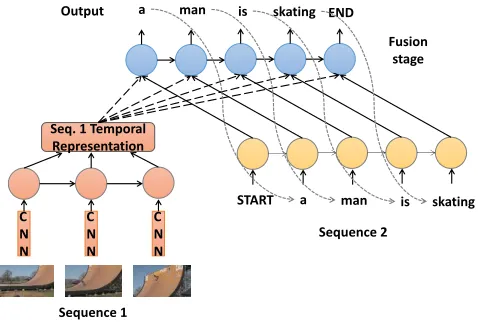
Fig 1. An illustration of FRMM architecture using a video description example .. 2

Fig 2. Architecture of image description model proposed by Karpathy et al. [13] 7 Fig 3. RCNN/BRNN based word and image feature vector embedding. [13] ... 8

Fig 4. Architecture of Neural Image Caption generator. [14] ... 10

Fig 5. LRCN variants: Unfactored and factored LRCN architectures. [9] ... 11

Fig 6. Fusion models proposed by Karpathy et al. [15] ... 12

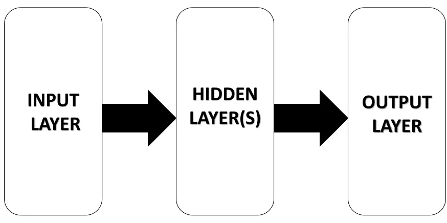
Fig 7. Basic architecture of an ANN with input, hidden and output layers. ... 14

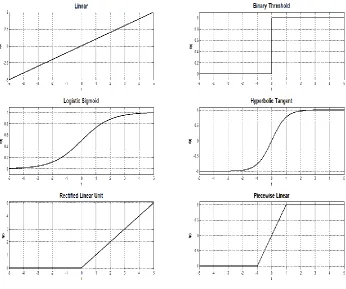
Fig 8. Plots of various activation functions. ... 18

Fig 9. Gradient descent illustration. [23] ... 25

Fig 10. A pictorial depiction of issues with small and large learning rates. ... 26

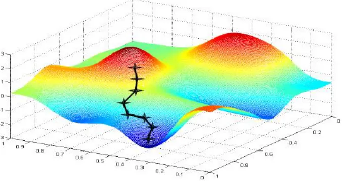
Fig 11. A scenario where the solution is stuck at a local minima. ... 28

Fig 12. Momentum helping weights from being stuck at a local minima. ... 29

Fig 13. Illustration of dropout applied to a ANN (a), resulting in (b). ... 33

Fig 14. Neuron's behavior during training and testing time with dropout. ... 34

Fig 15. A FNN with one input, one output and one hidden layer. ... 35

Fig 16. Comparison of FNN and CNN. [32] ... 40

Fig 17. Illustration of the receptive field concept for a 32x32x3 image. [32] ... 41

Fig 18. Output computation for CONV illustrated using a 5x5x3 input. [32] ... 45

Fig 19. Downsampling the output size through pooling. [32] ... 48

Fig 20. CNN architecture for a typical image classification problem. [32] ... 50

Fig 22. SRN architecture with one hidden layer. ... 54

Fig 23. Illustration of forward propagation in SRN. ... 55

Fig 24. Illustration of inability to capture long-term dependency using a SRN based activity classifier that uses video input. ... 59

Fig 25. Preserving long term dependencies using input and output gates. ... 60

Fig 26. The internal architecture of a LSTM cell. ... 61

Fig 27. Illustration of BPTT for a LSTM cell. ... 64

Fig 28. Images and corresponding captions from Flickr8k dataset. [40] ... 66

Fig 29. SRN predictions for RELU, tanh and sigmoid activations on Flickr8k. .. 68

Fig 30. Illustrations of FRMM architectures with image captioning examples. .. 72

Fig 31. Some of the accurate image descriptions generated by AFRMM. ... 80

List of Tables

Table 1. Evaluation of the performance for various activation functions in SRN

based architecture for Flickr8k. ... 66

Table 2. Comparison of performance between tanh and RELU in LSTM based

architecture for Flickr8k. ... 68

Table 3. Comparison of performance between tanh and PL in LSTM based

architecture for Flickr8k. ... 69

Table 4. Relation between word frequency threshold based vocabulary elimination

and performance in LSTM based architecture for Flickr8k. ... 70

Table 5. Evaluation of the performance of image description model with various

FRMM architectures on the MSCOCO dataset. ... 77

Table 6. Evaluation of the performance of image description model when image

feature descriptor is extracted from layers fc6, fc7 and fc8 of the CNN on the MSCOCO

dataset. ... 78

Table 7. Performance of image description model with two-layered LSTM

architectures in each stage. ... 78

Table 8. Comparison of our approach with other proposed methods using BLEU

and METEOR scores for MSCOCO dataset ... 79

Table 9. Comparison of our approach with other proposed methods using BLEU

Chapter 1

Introduction

Accurate text annotation of image and video content enables more efficient search and

retrieval, can aid visual understanding in medical, security, and military applications,

and can even be used to describe pictorial content to the visually impaired.

Uncertainties about salient content, main subject detection, object recognition, action

detection, and scene understanding make this a challenging problem. Despite the

difficult nature of this task, computer vision and natural language processing

researchers have made significant strides in this area. This thesis work builds upon

these previous successes, and introduces a new framework that simultaneously

Fig 1. An illustration of FRMM architecture using a video description example

In the past five years, supervised convolutional models have forever changed the

computer vision and machine learning landscape. Due to the recent introduction of

large supervised datasets [1] and accelerated training models using Graphic Processing

Units (GPUs) [2], the traditional pairing of hand crafted low level vision features with

complimentary classifiers has been bested by Convolutional Neural Networks (CNNs)

[3]. CNNs are deep feed forward networks based upon a hierarchy of abstract layers

which simultaneously learn the low level features and classifier. These networks have

been shown to equal the performance of neurons in the primate inferior temporal

cortex, even under difficult conditions such as pose, scale, and occlusions [4]. CNNs

have won competitions in traffic sign detection, house number detection, handwriting

recognition, pedestrian detection, object recognition, speech recognition, breast cancer

detection, and many more.

A number of works have extended the image recognition framework to video

frames. Motivated by the need to learn temporal sequences, Recurrent Neural

Networks (RNNs) enable solutions to basic problems such as activity recognition and

C N N C N N C N N Fusion stage Sequence 1 Sequence 2 a

Output man is skating END

START a man is skating Seq. 1 Temporal

object trajectory prediction. In practice, RNNs suffer from vanishing and/or exploding

gradients- a problem where the backpropagation of an error signal over several

iterations will diminish quickly (e.g. several successive multiplies by a value < 1) or

explode quickly (e.g. several successive multiplies by a value > 1). The Long Short

Term Memory (LSTM) models [5] solved the gradient problem by replacing the

traditional artificial neuron with a memory cell containing long and short term

non-linear capabilities. The LSTM’s incredible power was first realized in the speech and

natural language processing domains [6], and more recently to the annotation of image

and videos [7-12]. LSTMs are a natural fit for temporal sequences of varying lengths

and can be trained using standard back propagation.

1.1.

Contributions

Our architecture takes advantage of these powerful CNN and LSTM architectures and

uses a multi-modal shared representation for learning a combination of data sequences.

In this thesis work a set of end-to-end trainable fusion based recurrent architectures for

multi-modal learning, called FRMMs, are introduced. These FRMMs are used in the

context of image captioning where image features and vocabulary are learned in

independent stages and then mapped to a shared representation in the fusion stage. This

allows for the fusion of multiple arbitrary length sequential streams, which to the best

of my knowledge, is the first study of its kind. The independent stages also allow for

doing away with the use of shared parameters for learning different modalities and

features of that modality. In addition, this thesis work analyzes the impact of various

activation functions on the performance of RNNs and LSTMs and the impact of

vocabulary size on the effectiveness of the image description model. Furthermore, the

generic nature of the FRMM based architectures allow them to be deployed for a

multi-modal learning problem. Fig 1 shows an illustrative example of an FRMM model that

is deployed for video description.

1.2.

Overview of Thesis

The rest of the thesis is organized as follows. Chapter 2briefly describes some recent

research works in this area that have motivated this work and how this work adapts and

builds upon those techniques. Chapter 3introduces Artificial Neural Networks (ANN).

Chapter 4, Chapter 5 and Chapter 6 cover specific ANN architectures namely Feedforward

Neural Networks, Convolutional Neural Networks and Recursive Neural Networks.

Chapter 7 presents the findings for activation function and vocabulary size based

experiments while Chapter 8 introduces the FRMM architectures and compares its

performance with other state of the art image description works. The conclusions and ideas

Chapter 2

Motivation from previous work

Recent research [9, 13-15] has demonstrated state-of-the-art image captioning results using

deep learning technique. These methods analyze visual information, recognize and classify

objects and actions, and describe both still and video frames through captions. All these

works use a supervised learning scheme where images with corresponding captions are

used to train the network. Convolutional Neural Networks (CNNs) are deployed for visual

feature extraction and recursive neural network based architectures, either a simple

recursive network or a Long-Short Term Memory (LSTM) based architecture are used to

learn the language model and then generate descriptions. This thesis work draws inspiration

from their work, adapts some of the concepts used in the works and builds upon those

techniques to help overcome their limitations in an attempt to improve results. This section

briefly walks the readers through the approaches employed in the aforementioned

researches and describes the concepts adapted.

The first work being described in this section is by Karpathy et al. [13]. The basic

architecture for his model is shown in Fig 2. It uses a CNN that has been pretrained on

ImageNet [16] and fine-tuned on the datasets in ImageNet challenge [1]. In addition a

Simple Recurrent Network (SRN) is used to function as a caption generator. During

training the SRN is fed the image feature descriptor from the CNN in addition with the

keyword START at the first time instance, followed by each word in the ground truth image

caption from the training data at every time instance, along with the hidden state from the

previous time step. After training with enough exemplars, the SRN learns the language

semantics and predict the next word with a good accuracy based on either the previous

word or the image features through the weight updates. During testing, the image feature

descriptor extracted from the CNN is used as the first input to the SRN along with the

keyword START. The first word of the image caption is predicted based on the image

feature descriptor. The next prediction is made based on the previous prediction as input

along with the previous hidden state. The process continues until the end of sentence has

been encountered. Fig 2 demonstrates how the proposed architecture makes a prediction

Fig 2. Architecture of image description model proposed by Karpathy et al. [13]

Before the training and testing, Karpathy preprocessed the words by mapping them

into the same vector space as the image feature vector extracted from the CNN such that

the dot product of a word vector with its corresponding image vector is maximized. This

has been achieved through an RCNN as proposed by Girshick et al in [17], which identifies

the top nineteen regions/objects in an image and generates twenty image feature vectors by

passing these nineteen regions along with the entire image through a CNN. A SRN

architecture, called Bidirectional Recursive Neural Network (BRNN) [18] is used to map

each word into the same vector space as the image feature vector based on the contextual

information surrounding the word in both directions and the feature vector of the word’s

Fig 3. RCNN/BRNN based word and image feature vector embedding. [13]

This is illustrated in Fig 3, where a picture of a dog catching a frisbee is passed to

the RCNN. The example has three regions of interest: dog, frisbee and the entire image.

The words dog, catch and leaps correlate well with the image feature vector of dog,

maximizing the image-sentence score, which is the dot product of image feature vector and

word vector. Similarly, the image feature vector frisbee has a high correlation with the

word frisbee. Higher scores are indicated in the image with lighter shades, while darker

shades indicate lower image-sentence scores. Because of this preprocessing step for word

vectors and the freezing of all the layers in CNN, which is the image feature extracting

stage, this model is not end-to-end trainable. Also, while multi-modal embedding is an

important start as other researches show, learning it offline through a separate model is

The second research work that is very relevant to this thesis research is the Neural

Image Caption Generator (NIC) by Vinyals et al. [14]. It is similar to [13] in that it uses a

CNN, mapping the word vector into the same dimensional vector space as the image vector.

The difference is that this model is end-to-end trainable and does the word vector

(𝑆0 𝑡𝑜 𝑆𝑁−1) embedding into image feature vector space by learning the weight vector

𝑊_𝑒within the NIC. It also uses a LSTM architecture in place of a SRN architecture to

improve performance and a beam search algorithm that keeps track of k possible image

captions and then picks the sentence with the least loss, which is the absolute value of sum

of log probabilities of each word in the caption given the previous words. This has

apparently helped them improve the BLEU scores of NIC by an average of two points.

They also use a different CNN, a variant of GoogLeNet [19], the best performing model

from the ILSRVC 2014 classification competition. Their results demonstrate advantages

LSTM based networks and end-to-end training offer, over SRNs based caption generators

and the superfluousness of having a separate BRNN for a word vector embedding into an

image vector space. Fig 4 shows the architecture of CNN and LSTM based NIC generator

Fig 4. Architecture of Neural Image Caption generator. [14]

The third research work in image description using deep learning is the Long-term

Recurrent Convolutional Networks (LRCNs) proposed by Donahue et al. [9]. It shares the

similar features such as end-to-end trainability and CNN/LSTM based caption generators.

It is different from the previously discussed research in the sense that it doesn’t constrain

the word vector to be in the same dimensional vector space as the image feature vector and

it introduces interesting multi-layered LSTM architectures. It employs a pre-trained CNN

architecture on ImageNet dataset [16] as proposed by Krizehvsky et al. in [2], and

fine-tunes the fully-connected layers of the CNN using the end-to-end trainability of LRCN

architecture. In addition to LRCNs that have just a single layer LSTM, similar to NIC, it

has two layered LSTM architectures where either both layers are used to train on both

image and word vectors while the first layer is exclusively reserved for the word vector

inputs (factored version). These LRCN variants are depicted in Fig 5.

Fig 5. LRCN variants: Unfactored and factored LRCN architectures. [9]

The results of LRCN indicate that factored LRCN yields better captions than

unfactored LRCN. This has led to the idea of having independent learning stages for image

feature vectors and word vectors in this research, in order to avoid sharing parameters for

disparate modalities. On top of this independent learning stages for each modality, a LSTM

Fig 6. Fusion models proposed by Karpathy et al. [15]

The concept of fusion and combining learning from two independent streams has

been borrowed from [15] where visual information from two distinct set of frames is fused

temporally into one layer. This work extends that concept of fusion of disparate input

modalities and uses the LSTM based fusion architecture as multi-modal applications often

have a temporal dependency on output from previous time steps. Fig 6 shows the fusion

models where the red, green, blue and yellow boxes indicate convolutional, normalization,

Chapter 3

Artificial Neural Networks

Artificial Neural Networks (ANNs) are a computer emulation of a simplified model of the

billions of neurons in the human brain. Each node within an ANN mimics a neuron of the

human brain and is also often referred to as a neuron. This chapter only talks about the

functionality of ANNs in the context of supervised learning where the input and

corresponding outputs from the training data are used to help the network understand the

relationship between input and output. In order to recreate the functionality of the nervous

system and capture the relationship between input and output, each node in an ANN is

connected to multiple input and output nodes through weighted connections. These weights

are learned over time, during backpropagation where the ANN modifies the weights based

on how closely the predicted outputs match the ground truths of the testing data. This

process will be elaborated in the following sections. The firing of the neurons in the brain

is caused by sharp electrical spikes. This firing is recreated in ANNs through the use of

non-linear activation functions like sigmoid, tanh and rectified linear units within each

node. A collection of such nodes where each node is connected to a number of other nodes

forms an ANN. The nodes that are connected to sensory and responsive parts of the system

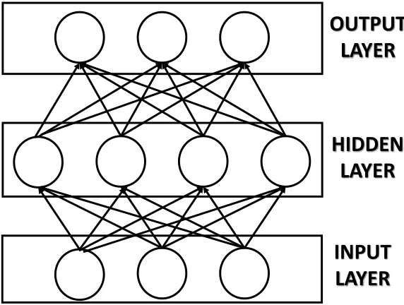
other nodes in the network are called hidden nodes and form the hidden layer. Fig 7

illustrates the basic architecture of an ANN. Based on how the nodes within each layer of

an ANN interact with one other, ANNs can be broadly classified into Feedforward Neural

Networks (FNN) and Recurrent Neural Networks (RNN). In the following discussion, the

word neuron refers to a node in an ANN and not a neuron of the human brain and the terms

node and neuron will be used interchangeably.

Fig 7. Basic architecture of an ANN with input, hidden and output layers.

3.1.

Activation Functions

The previous sections talk about using activation functions to modulate inputs, but they

don’t describe what these functions are. This section describes the most common activation

functions used in ANNs.

INPUT

LAYER

OUTPUT

LAYER

HIDDEN

Linear

A linear activation function, as the name suggests is a linear function of the form:

𝒇(𝒕) = 𝒄 ∗ 𝒕 (𝟏)

where c is a constant. Linear activation functions are seldom used in practice, and were

used only during the infancy of neural computing, as an ANN using a linear activation can

be reduced to a linear multi-variate regression model and thus can’t be used to generate

linear boundaries between classes. The activation functions that follow are all

non-linear.

Binary Threshold

The binary threshold is a step function and is helpful in classifying the inputs into two

distinct classes. It is mathematically represented as shown in (2). The numbers p and n are

real numbers usually with values 1 and -1/0 while threshold is usually a positive real value.

𝑓(𝑡) = {𝑝 𝑓𝑜𝑟 𝑡 ≥ 𝑡ℎ𝑟𝑒𝑠ℎ𝑜𝑙𝑑

𝑛 𝑓𝑜𝑟 𝑡 < 𝑡ℎ𝑟𝑒𝑠ℎ𝑜𝑙𝑑 (2)

Binary Threshold is one of the first non-linear activation functions to be used in

ANNs called perceptrons. However as it is a non-differentiable, it is no longer used in

ANNs. The importance of a differentiable non-linear activation function will become more

S-shaped non-linear functions like logistic sigmoid and hyperbolic tangent are employed.

They are non-linear and differentiable.

Logistic Sigmoid

The logistic sigmoid, simply referred to as sigmoid, is a non-linear S-shaped function

defined by the mathematical equation:

𝑓(𝑡) = 1

1 + 𝑒−𝑡 (3)

It is a very popular activation function and has been widely used in many ANN

solutions. As it can be seen, with a value of 0.5 at t=0, this function is not zero centered

and is always positive, leading to both positive and negative exemplars having positive

outputs in classification paradigms. While this can be rectified with the right bias, it would

be preferable for an activation function in classification models to have positive values for

positive exemplars and negative values for negative exemplars. Hence as sigmoid, is not

zero-centered and for other reasons discussed in the following sections, like the vanishing

gradient problem, this activation function is no longer favored and is being replaced by

hyperbolic tangent and rectified linear unit.

The hyperbolic tangent (tanh) is a non-linear S-shaped function like logistic sigmoid, which

unlike sigmoid is zero-centered, with a steeper rise which can be especially helpful in

classification models to reduce the number of misclassified samples. The tanh function is

differentiable, unlike the binary threshold. Mathematically, the hyperbolic tangent is

represented as:

𝑓(𝑡) =𝑒

2𝑡_{− 1}

𝑒2𝑡_{+ 1} (4)

While tanh offers many benefits over the previously discussed activation functions,

it is still susceptible to vanishing gradient problem, although much less likely than sigmoid.

Rectified Linear Units (RELU)

A rectified linear unit is a non-linear, differentiable activation function that is not as

susceptible to the vanishing gradient problem, an issue that shall be discussed in the

following sections. Mathematically a RELU is represented as

𝑓(𝑡) = max(0, 𝑡) (5)

RELU, is the most popular activation function in deep neural networks, an ANN

with many hidden layers, due to its ability to circumvent the vanishing gradient problem.

A piecewise linear function is a non-linear, S-shaped, differentiable activation function

which may not be as susceptible to the vanishing gradient problem. Mathematically a

piecewise linear function is represented as

𝑓(𝑡) = {

1 𝑖𝑓 𝑡 > 1 𝑡 𝑖𝑓 − 1 ≤ 𝑡 ≤ 1

−1 𝑖𝑓 𝑡 < −1

(6)

Fig 8 shows all the activation functions discussed so far in the same order as discussed

3.2.

Cost Functions

In order to determine the accuracy and efficiency of an ANN, the predicted results need to

be compared to the ground truth during the training process and the network needs to be

penalized every time the predicted output is incorrect. This is achieved through employing

a cost function, c, that determines the amount by which the network needs to be penalized.

This section describes the most common cost functions used. Before various cost functions,

also referred to as loss functions, are introduced, it is important to describe the properties

a cost function must satisfy. Firstly, a cost function should always produce a non-negative

result, as knowing whether the prediction is greater than or less than the target value doesn’t

convey much information about the accuracy of the system. It’d be more beneficial to

understand how close or far away our predicted output is from the desired output. Secondly,

the cost should decrease and approach zero when the predicted output is close to the target

output, i.e. ground truth for that particular input sample and increase when the predicted

output moves away from the target output.

Mean Absolute Error

The mean absolute error is the mean of sum of absolute difference between target output

and predicted output over all the training samples. The absolute difference, highlights the

magnitude of difference between the prediction and the ground truth, satisfying both the

𝑐 = 1 𝑆∑ |𝑦

𝑖_{− 𝑡}𝑖_| 𝑆

𝑖=0

(7)

where c is the total cost incurred by the network through penalty, S is the number of training

samples and 𝑦𝑖, 𝑡𝑖 are the predicted output and target output for ith_{training sample. Mean}

Absolute Error is mainly used in ANN models designed for prediction and regression

analysis.

Least Squares

The least squares method calculates the mean of the sum of the squared difference between

target output and predicted output over all the training samples. Using the square of the

difference ensures both positive and negative errors are all converted to positive values,

and the squared difference exponentially increases the cost when the prediction moves

further away from the target and vice versa. The least squares function is given by the

equation:

𝑐 = 1 𝑆∑(𝑦

𝑖_{− 𝑡}𝑖₎2 𝑆

𝑖=0

(8)

where c is the total cost incurred by the network through penalty, S is the number of training

samples and 𝑦𝑖_{, 𝑡}𝑖 _{are the predicted output and target output for i}th_{training sample. The}

predictive applications, and is very often favored over mean absolute error, due to its

convex shape offering a single minima for linear regression models and thus guarantees a

closed-form solution. Although there might be multiple minima for multivariable nonlinear

models that use least squares, leading to the problem of the parameters being stuck at one

of the local minima, this can usually be avoided by choosing the right values for training

parameters like learning rate and momentum, which shall be discussed in further sections.

Hinge loss

Hinge loss is a cost function that is used almost exclusively for classification problems. In

order to devise a cost function for classification models, it is first essential to understand

how the output of a classifier is interpreted. In the context of ANNs it is conventional to

assume that the node of the output layer, where each output node represents a particular

class in the multi-class model, with the highest output value indicates the class the input

sample belongs to. With this understanding, it can be said that whenever a node has a value

greater than the actual output, the network needs to be penalized. Also, establishing a safety

margin, that dictates the minimum difference between the actual output and the output of

all the other nodes, and penalizing whenever this condition is not met, ensures that there

wouldn’t be any nodes whose output despite being less than the actual output is too close

it to be completely ignored. The loss function can be mathematically written as:

where ∆ is the safety margin, 𝑦𝑗 is the output for the ground truth node, and 𝑦𝑖 represents

all other nodes other than node j. The loss is zero when node’s i output are a distance of ∆

or less than node j. The hinge loss function also goes by the name multiclass SVM loss, as

this function was first used in multiclass SVM models.

Cross entropy

Cross entropy, also referred to as softmax loss, is a cost function used by classification

problems. It is an improvement over the hinge loss function in that it generates scores that

are more meaningful and easier to interpret by using probability of the input belonging to

each class as the output. For this reason softmax is the most commonly encountered loss

function for classification problems. Softmax converts the large +/- range class scores

generated by a classifier into values between 0 and 1 such that the sum of the values is one.

This can be achieved by using the softmax function for all output values. The softmax

function is given by:

𝑠𝑜𝑓𝑡𝑚𝑎𝑥(𝑦𝑗) = 𝑒

𝑦𝑗

∑_𝑆 𝑒𝑦𝑖

𝑖=1

(10)

Now that the outputs are squashed to values between 0 and 1, the rules for

penalizing the network can be established. Whenever the network is not very confident

about the input sample belonging to the desired class, i.e. whenever the probability of the

desired class is less than 1, the network needs to be penalized. This can be achieved by the

𝑐 = −1

𝑆∑ log (𝑠𝑜𝑓𝑡𝑚𝑎𝑥(𝑦

𝑗₎₎ 𝑆

1

(11)

where S is the number of classes. As it is evident from the above equation, whenever the

probability is equal to one the cost incurred becomes zero and when the probability is less

than 1 there is a positive cost incurred. Cross-entropy satisfies both the properties of a cost

function and provides more meaningful insight than hinge loss.

3.3.

Determining the weights

3.3.1 Initializing the weights

The best way to initialize weights in an ANN is an area of active research in itself. Thus

this document shall neither comprehensively cover the topic nor compare and contrast one

method with another. However, the most commonly used techniques are briefly discussed

in this section. When training an ANN from scratch, it is very important to ensure that all

weights are not initialized to zero, as that would lead the output of any input to remain

unchanged. This problem can be avoided by using random weight initializations, which

usually use samples from a zero mean unit standard deviation Gaussian function. One

common practice is to use small weights, to ensure that the network isn’t initially highly

biased towards any particular subset of inputs as this would slow down the process of

convergence. It is also common to normalize variance for the output of each node to ensure

all nodes initially have an equal impact on determining the output. This normalization has

inputs and m outputs, this can be achieved by either scaling the weights with √1

𝑛, √ 2 𝑛+𝑚

[20] or √2

𝑛 for ANNs that use a ReLU activation function [21]. To avoid delays in

convergence due to bad weight vector initializations by using a batch normalization layer

before non-linear activations are applied to the output as proposed in [22]. If a pre-existing

ANN architecture with an optimal solution that has been trained on a similar dataset exists,

then transfer learning should be used. Transfer learning uses a good weight initialization,

ultimately enabling faster convergence and higher accuracies.

3.3.2 Updating the weights

Once the performance of the ANN model has been determined by using one of the

aforementioned cost functions, the next step is to update the weights so as to reduce the

penalty incurred from the cost function. The procedures mentioned in the following

discussion describe the methods through which the weights can be updated so as to

converge to the minimum penalty point quickly.

Stochastic Gradient Descent

Derivatives are used to analyze the change in a dependent variable, like cost incurred, with

respect to a change in an independent variable, such as weights in an ANN. As a typical

network has many weights, the effect of change in each weight on the cost needs to be

considered using partial derivatives (gradients). When the gradient is positive, it implies

the cost increases with an increase in that weight parameter; hence the weight parameter

implies that the cost decreases with an increase in the weight parameter; hence the weight

parameter needs to be increased proportionally to the gradient. This process of descending

towards the optimal minimum by constantly taking steps proportional to the negative of

the gradient is referred to as gradient descent. Fig 9 illustrates how gradient descent leads

the model to the optimal solution.

Fig 9. Gradient descent illustration. [23]

Parameter update based on gradient descent for a weight 𝑊𝑖𝑗in the network can be

represented as

Δ𝑊_𝑖𝑗(𝑡) = 𝜂 𝜕𝑐

𝜕𝑊_𝑖𝑗 (12)

where c is the cost incurred and 𝜂 is the learning rate that decides the pace at which the

weights are updated. If 𝜂 is too high then the gradient descent step might be too large,

making the model miss the optimal solution. This can be identified by looking at the cost

function plot. If the cost oscillates or increases it is an indication of the learning rate being

too high. On the other hand if 𝜂 is too low, it takes a longer time for the model to reach the

optimal solution. The reason for large learning rate resulting in divergence and small

learning rate resulting in slow convergence is illustrated in Fig 10.

Fig 10. A pictorial depiction of issues with small and large learning rates.

Mini-batch Gradient Descent

As opposed to stochastic gradient descent, where the weights are updated based on the

gradient for each input, mini-batch gradient descent evaluates the cumulative loss and

gradients of weights over a collection of input samples, often referred to as a mini-batch,

and updates the weights once for each mini-batch. The cumulative gradient updates, just

Small learning rate

leads to a slow convergence

involve adding up of gradients obtained from various inputs. This helps reduce the number

of times the weights are updated before convergence. Although it might be

counter-intuitive at first, this update method also helps stabilize and improve the accuracy of the

predictions in the classification paradigm as the network is provided exemplars from

various classes before each update. As the update decision is not solely based on an input

that belongs one of the many classes involved, the updated weights aren’t just modified in

favor of just one class, or worse one outlier data sample. Thus, very often an increase in

the hyperparameter batch size, the number of samples involved in each mini-batch update,

is recommended whenever there is a considerable variation in accuracy between

consecutive iterations. When the batch size is equal to all the samples in the training set,

the gradient update scheme is referred to as batch gradient descent and when the batch size

is 1, the gradient descent method becomes stochastic gradient descent. On a side note, when

all the training samples are used to update the weights exactly once, it is called an epoch.

A typical ANN needs to be trained for multiple epochs before it converges.

Momentum

Until this point, the focus has been mostly on analyzing convex functions with one

minimum for the entire function. However, it is not uncommon for the cost functions to be

have multiple local minima along with the global minimum that provides the optimal

solution. Fig 11 depicts this scenario. In such a case, based on the initialization of weights,

the network might be stuck at one of the local minima during the learning and can’t

converge to the optimum solution. This is due to the fact that gradient descent is a greedy

rate is too slow. One way to avoid converging to a local minima is by taking a look at the

previous amount by which the weight was previously changed Δ𝑊_𝑖𝑗(𝑡 − 1). [23] proposes

a solution using this technique by modifying (12) to include the gradient of the parameter

during the previous iteration. 𝛼 is a hyperparameter called momentum.

Δ𝑊𝑖𝑗(𝑡) = 𝜂 𝜕𝑐

𝜕𝑊𝑖𝑗+ 𝛼Δ𝑊𝑖𝑗(𝑡 − 1) (14)

Fig 11. A scenario where the solution is stuck at a local minima.

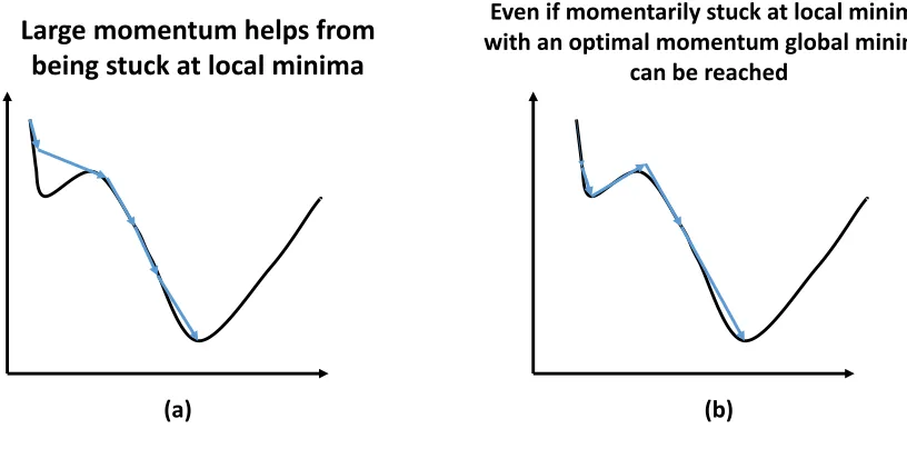
However, when first employed in [23], the aim of adding the momentum term was

to speed up the training thus leading to a faster convergence without leading to oscillations,

which happens by increasing the learning rate. But the same has been shown to overcome

converging to a local minima by choosing an optimal momentum parameter. This can

happen in one of two ways. Adding the momentum term might cause the gradient to skip

over the local minima thus avoiding it. If not, despite the partial derivative of the cost

historical weight update parameter 𝛼Δ𝑊_𝑖𝑗(𝑡 − 1) makes Δ𝑊_𝑖𝑗(𝑡) non-zero causing the

weight to move away from the local minima. This is illustrated in Fig 12.

Fig 12. Momentum helping weights from being stuck at a local minima.

Scenario (a) avoids local minima by moving over it, scenario (b) moves away from local minima despite landing there, due to the momentum.

Adaptive learning rate

The discussion so far has treated the weight update hyperparameter learning rate 𝜂, as a

constant. However, as illustrated in Fig 10 picking a small learning rate, while helps us

reach the global minima, takes a long time to converge and large learning rates might lead

to divergence. However, a larger learning rate could be used initially during the training to

reach closer to the minima sooner and then the learning rate could be lowered over time to

avoid divergence. Thus having an adaptive learning rate helps us reach the global minimum

with a faster convergence time. The adaptive learning rate schemes can be further classified

based on whether the learning rate is changed globally or individually for each parameter. Large momentum helps from

being stuck at local minima

Even if momentarily stuck at local minima with an optimal momentum global minima

can be reached

The most common global update schemes include reducing the learning rate by a scaling

factor when validation accuracy stops improving or reducing the learning rate with an

exponential decay for each iteration. Per-parameter update methods on the other hand, rely

on the gradient to determining the learning rates. Weights that receive high gradients have

their learning rates lowered more aggressively than weights that receive lower gradients.

This is because large gradients indicate large learning rates as shown in Fig 10. RMSprop

[24] and Adagrad [25] are two of the most widely used and effective adaptive learning rate

schemes in the same order.

3.4.

Avoiding overfitting

Overfitting is the phenomena in which an ANN learns the intricate input output relations

that are specific only to the training data and thus ceases to capture the generic relation

between inputs and outputs. In other words, the ANN starts to impose additional

restrictions and constrains learned from a subset of data, that are not always satisfied all

data members, which should at all costs be avoided. A good example of this would be an

ANN that expects a car to have four doors and a roof as it has been trained mostly on

images of cars with four doors and a roof. Overfitting can be avoided in more than one

way. Three of the most popular techniques are discussed here. The first way is to constrain

the weights from having higher values thus preventing any particular subset of inputs to

have a high weight in determining the outputs through a technique called regularization.

The second technique uses multiple network architectures to be trained on the same data

and pick the final output through an averaging or voting scheme, using an ensemble or a

data augmentation techniques. The idea is to show more variations of inputs to the network.

Each of these methods are briefly discussed below.

Regularization

Regularization is a technique used to prevent networks from overfitting to their training

data. While there isn’t much theoretical evidence to demonstrate how regularization

prevents overfitting, it has been empirically proven that the networks which employ

regularization techniques, perform better over their counterparts on unforeseen data.

Regularization ensures that the network can’t learn the noise patterns from the training

dataset. Regularization can be incorporated into the training with either L1 or L2

regularization schemes discussed below.

L2 regularization

L2 regularization scheme incurs a cost on each of the weights in the network, the further

away a weight value is from 0, the greater the cost. In addition, for linear classification

models like SVM, where it is usual for many possible solutions to exist, L2 regularization

reduces the ambiguity and the number of possible solutions by imposing penalty on higher

weights, forcing them to have weights whose magnitude is closer to zero. The penalizing

is implementing by including a term, called the regularization term, in the cost functions

described by (7) through (11). The regularization term adds the product of sum of all the

squares of the weights in the network and a hyperparameter λ is used to control the amount

𝑐 = −1

𝑆∑ log (𝑠𝑜𝑓𝑡𝑚𝑎𝑥(𝑦𝑗))

𝑆

1

+ 𝜆 ∑ 𝑊2

∀𝑤

(15)

L1 regularization

L1 regularization also reduces overfitting through constraining the weights from becoming

too large just like L2 regularization. However, instead of making the penalty proportional

to the sum of squares, it makes the penalty proportional to the sum of absolute weights.

The L1 is generally less susceptible to large outliers, but does not have an exact gradient.

The cost function of a network that uses L1 regularization techniques can be written as:

𝑐 = −1

𝑆∑ log (𝑠𝑜𝑓𝑡𝑚𝑎𝑥(𝑦𝑗))

𝑆

1

+ 𝜆 ∑ |𝑊|

∀𝑤

(16)

Dropout

Dropout [26] is a technique inspired by neural network ensembles, a technique that uses

multiple network architectures to be trained on the same data and pick the final output

through an averaging or voting scheme as mentioned in [27]. Dropout has gained a great

deal of popularity in the past few years in the field of deep neural networks ever since they

have been introduced in [2]. The idea is to drop hidden nodes in the network randomly with

a probability of ‘p’ in each iteration during the training. A common value of p is typically

0.5. The network learns with the help of the hidden nodes that remain. This procedure

creates multiple “sub-networks” during the training phase. Thus the training procedure is

multiple architectures manually and training each of them separately. The lack of one

pre-defined architecture for the entire training phase also eliminates the possibility of

co-dependence of weight updates during backpropagation leading to unwanted weight

convergences as not all weights and biases are updated during each iteration. Dropout also

serves as an alternative to regularization by reducing the impact of any particular node on

the output. This process is illustrated in Fig 13, where the network on the left side shows

how the architecture of a typical ANN on the left changes when nodes are randomly

dropped out on the right.

Fig 13. Illustration of dropout applied to a ANN (a), resulting in (b).

During the testing phase, the weights need to be scaled by a factor of ‘p’ as all the

hidden nodes will be used. This scaling gives the average consensus among the “ensemble

of sub-networks” during the testing. Fig 14 shows how each neuron acts during the training

and testing phases in a neural network when using dropout.

Fig 14. Neuron's behavior during training and testing time with dropout.

Data Augmentation

Data augmentation is a technique that has been heavily utilized in both computer vision

and speech research to artificially increase the size of the training data [2], [9], [15], [28],

[29]. This increases the network’s accuracy, as the network gets to see more variations of

the inputs. The size of the training data is usually increased by introducing noise into the

existing training data. For images and videos, the inputs are randomly cropped, flipped

horizontally and vertically and the parameters like brightness, contrast are played with. For

speech recognition works, random noise functions like Gaussian noise are introduced to

the speech inputs. As more training data avoids overfitting, data augmentation has led to

the development of better performing networks.

p w1

w2

w3 _p*w1

p*w2

p*w3

At training time a node can be dropped out with a probability of p

Chapter 4

Feedforward Neural Networks

A Feedforward Neural Network (FNN) is an ANN where the output of neurons in a given

layer can be fed as inputs only to the neurons in the next layer. As forward connections are

the only acceptable connections for the neurons, they are feed forward in nature. Very

often, a FNN is also referred to as a Multi-layer Perceptron (MLP) due to their similarity

to perceptrons . Fig 15 depicts a FNN with one input layer, one output layer and two hidden

layers.

Fig 15. A FNN with one input, one output and one hidden layer.

OUTPUT

LAYER

HIDDEN

LAYER

4.1.

Forward propagation in FNN

In forward propagation or forward pass, the input patterns are fed to the input layer. The

outputs of the input layer are propagated to the next layer and the propagation of the outputs

from one layer to the next is continued until the output layer where the output prediction is

obtained.

Consider a FNN with the input layer containing M nodes, one hidden layer

containing H nodes, an output layer containing N nodes, and the usage of non-linear

activation functions after each node. Let 𝑊 𝑎𝑛𝑑 𝑊′ be the input to hidden and hidden to

output weight vectors respectively such that 𝑊_𝑚ℎ and 𝑊_ℎ𝑛′ represent the weights of

connections from mth input node to hth hidden node and hth hidden node to nth output node

respectively such that 0 ≤ 𝑚 ≤ 𝑀, 0 ≤ ℎ ≤ 𝐻 𝑎𝑛𝑑 0 ≤ 𝑛 ≤ 𝑁. Let x and y be the input

and output vectors of cardinality M and N respectively and 𝑖_ℎ, 𝑜_ℎand 𝑎_𝑛 be the net input

and net output of the hidden node h and net input of output node n. Then the output at each

node of the output layer can be calculated using the following set of equations.

𝑖_ℎ = ∑ 𝑊_𝑚ℎ∗ 𝑥_𝑚 (17)

𝑀

𝑚=0

𝑎_𝑛 = ∑ 𝑊_ℎ𝑛′ ∗ 𝑜_ℎ

𝐻

ℎ=0

(19)

𝑦_𝑛 = 𝑓(𝑎_𝑛) (20)

4.2.

Backpropagation in FNN

Back propagation is the process through which the penalty incurred from the cost function

is distributed to the parameters of the network. It has been stated in the previous sections

that the parameter updates are done by using gradient descent. However, the partial derivate

of the cost function with respect to all the weights in the network need to be known to

update each of the weight parameters. Since its introduction in [31], back propagation has

been widely used in artificial neural networks to update the parameters during training

stage. The process is similar to gradient descent, but is more general in that it is applicable

to multi-layered FNNs. Gradient descent is a special case of backpropagation for an ANN

with a single layer. The cost function, depends on the output of the output layer, the output

layer in turn depends on the hidden layer(s), which is in turn fed by the input layer. So,

there exists an indirect relation between all the weights and the cost function and the partial

derivative of the cost function with respect to the weights can be determined using the

chain rule. The partial derivatives of the cost function with respect to some hidden to output

and input to hidden weights say 𝑊_ℎ𝑛′ and 𝑊𝑚ℎare given by

𝜕𝑐 𝜕𝑊_ℎ𝑛′ =

𝜕𝑐 𝜕𝑦∗ 𝜕𝑦 𝜕𝑓∗ 𝜕𝑓 𝜕𝑎𝑛

∗ 𝜕𝑎𝑛

𝜕𝑐 𝜕𝑊_𝑚ℎ=

𝜕𝑐 𝜕𝑦∗

𝜕𝑦 𝜕𝑓∗

𝜕𝑓 𝜕𝑎_𝑛∗

𝜕𝑎_𝑛 𝜕𝑜_ℎ∗

𝜕𝑜_ℎ 𝜕𝑓 ∗

𝜕𝑓 𝜕𝑖_ℎ∗

𝜕𝑖_ℎ

𝜕𝑊_𝑚ℎ (22)

As it can be noticed from the above mathematical equations, calculating the

gradient descent with respect to individual weights involves backward propagation of error

obtained from the gradient of cost with respect to all the intermediate parameters that might

have contributions from the respective weights and hence the name back propagation. Once

these gradients of the cost function are computed with respect to the weights all that is left

Chapter 5

Convolutional Neural Networks

Convolutional Neural Networks (CNNs) are a specific form of FNNs that explicitly assume

the inputs to the network be structured samples, such as audio signals or image pixels which

can be filtered. These architectures typically focus on solutions for computer vision

applications, like classification, localization and segmentation of images and videos. So far

it has been assumed that layers in FNN are fully-connected, thus making each input

contribute to the output of all hidden layers. If a fully-connected FNN were to be used for

an application that uses an input from a VGA camera, whose standard resolution would be

640x480x3, then each hidden neuron shall have 921,600 weights for the connections

between the input and first hidden layer alone. An image of this dimension would require

the first hidden layer to have thousands of neurons. The model would have a billion weight

parameters just for the connections between input and hidden layer. This is unacceptable

both in terms of the computational power and memory requirements.

5.1.

Convolutional Layers

To prevent the networks from having too many parameters, the fully-connected layers are

replaced by convolutional layers in a FNN, leading to CNN models. In convolutional layers

(CONV), the hidden neurons are replaced with convolutional filters. Instead of solving for

neuron weights, we solve for a family of filters, each filter having its own weights. The

convolutional layers arrange the neurons in a 3D fashion using the height, width and depth

conventional FNN and a CNN. Each layer in the depth dimension, aka depth slice, of the

CONV layer is analogous to a filtered signal used for digital image processing, where each

filtered signal came from a learned filter, whose weights shall be learned during the training

process.

Fig 16. Comparison of FNN and CNN. [32]

5.2.

Hyperparameters used in CNNs

Understanding the following hyperparameters is necessary to design and fully comprehend

the way CNNs function. As depicted in Fig 16 and stated in the above discussion the

convolutional layers in CNN are three dimensional with some height, width and depth. The

3D volume of this convolutional network itself, which is just the number of neurons in the

5.2.1 Receptive Field

The filters in CNNs traverse the entire image using typical convolution. Because the filter

size is much smaller than the image, the number of weights we need to solve for is

drastically reduced. The spatial extent of the filters is determined by the receptive field

size. This process is inspired by the cognitive science behind the receptive fields in the

cortex of animals like cats and monkeys, where it has been demonstrated that nearby image

regions are mapped to the same or nearby neurons in their brains. This research has been

outlined in works [33-35]. Fig 17 depicts how a local spatial field in an input image is

mapped to a bunch of neurons. The reason as to why, it is being mapped to a bunch of

neurons would be clear after learning about the depth. It is very important to bear in mind

that, the receptive field cannot be selective about the depth of its input and has to operate

on the entire input depth. The local selection is only allowed along the width and height

spatial dimensions of the input.

5.2.2 Depth

The depth of the convolutional layer, determines the number of different neurons that

process the same receptive fields which is called the depth column, with a different set of

weights. For example, in traditional grayscale image processing, a filter may be of size

5x5. If the image were and color RGB image, the filter would be extended to 5x5x3. The

underlying idea is similar to connecting the same input node being processed by multiple

hidden nodes in traditional FNN architectures. The objective of having multiple neurons

processing the same receptive field is to identify and capture different features for the same

input region. Each filter applied to the input image (regardless of the depth), outputs a

single output plane. The number of filters, and thus the depth of the convolutional layers

are increased as the network moves from input to output as the network switches from

capturing simple features to more complex features within images. The depth of the

convolutional layer should not be confused with the depth of the CNN which is the number

of hidden layers in a CNN. Fig 16 and Fig 17 can also be used to illustrate the depth and

depth column respectively.

5.2.3 Stride

While the depth is determined by the number of input planes to a filter, the stride

determines the step value across and down the image as the convolution is performed. The

filter width, height, depth, and stride are used to construct the 3D convolutional layer. A

unit stride implies the need for introducing new depth columns for spatial regions of the

image that are a unit distance apart. The stride should be chosen carefully as low stride

the receptive fields leading to an increased redundancy in weights. Contrarily, higher stride

values yield lower resolution filtered images, at the cost of an increased risk in rapid loss

of vital information due to many input parameters contributing to a relatively smaller set

of parameters.

5.2.4 Zero padding

Zero padding involves padding zeros of mentioned size in all dimensions on either side of

the borders. For a spatial image with 2 dimensions, a zero padding of 1 involves padding a

row on top and bottom and a column on the left and right, thus increasing both the height

and width of the image by 2. Padding with a value greater than zero is a helpful method to

preserve the information on the borders of the image from vanishing through multiple

convolutions. It also preserves the spatial dimensions of the output from the convolutional

layers, often called the output volume. To understand and appreciate the need for

preserving the spatial dimensions of the output, one must be familiar with the pooling

layers of CNNs which shall be introduced in the following sections.

5.2.5 Output volume of CONV

The output volume of each CONV layer is the dimensions of the output of convolutional

layer, and is calculated using (23), (24) and (25). Let 𝐻_𝑖𝑛, 𝑊_𝑖𝑛, 𝐷_𝑖𝑛and 𝐻_𝑜𝑢𝑡, 𝑊_𝑜𝑢𝑡, 𝐷_𝑜𝑢𝑡be

the height, width and depth of input and output of a given convolutional layer. In addition,

let it be assumed that the hyperparameters receptive field, depth, stride and zero padding

size are given by𝐻_𝑟𝑓 x 𝑊_𝑟𝑓, 𝐾, 𝑆 and 𝑃 respectively. Then the output volume parameters

𝐻_𝑜𝑢𝑡 =𝐻𝑖𝑛− 𝐻𝑟𝑓+ 2 ∗ 𝑃

𝑆 + 1 (23)

𝑊_𝑜𝑢𝑡 = 𝑊𝑖𝑛− 𝑊𝑟𝑓+ 2 ∗ 𝑃

𝑆 + 1 (24)

𝐷𝑜𝑢𝑡 = 𝐾 (25)

The stride value 𝑆 needs to be picked such that 𝐻_𝑜𝑢𝑡, 𝑊_𝑜𝑢𝑡 are integral values.

5.3.

Parameter Sharing

In practice, there are a very few applications that evaluate pixel values at different locations

in an image with different filter values. Thus, a parameter sharing scheme would lead to a

great improvement in terms of the computational power, training time and memory

requirements. Now that there is only one set of weights per filter for all the pixel values,

the output of the CONV layer can be computed as a 3D convolution between the input and

the filter weights. This is actually the reason for naming this particular FNN architectures

as Convolutional Neural Networks.

5.3.1 Benefits

Based on what has been discussed so far the number of neurons in the convolutional layer

shall be 𝐻_𝑜𝑢𝑡∗ 𝑊_𝑜𝑢𝑡∗ 𝐷_𝑜𝑢𝑡 and each of these neurons has 𝐻_𝑟𝑓∗ 𝑊_𝑟𝑓∗ 𝐷_𝑖𝑛+ 1 weight

a stride of 5, a receptive field of 5x5, a filter size of 100, and a zero padding size of 0, the

output volume becomes 127x95x100 and each of the neuron in the CONV has 5*5*3+1,

i.e. 76 weights. Thus the convolutional layer shall have 91,694,000 weight parameters

which is very high.

The number of these parameters can be reduced by using the same weights for all

spatial co-ordinates within each filter. This leaves only the weight parameter computation

for 𝐷𝑜𝑢𝑡 filters each having 𝐻𝑟𝑓∗ 𝑊𝑟𝑓∗ 𝐷𝑖𝑛+ 1 weight parameters. This reduces, the

parameters of the illustrative model to 7600 from 91,694,000 which is a huge

improvement.Fig 18 shows output computation for a convolutional layer with inputs of

size 5x5x3, receptive field of 3x3, zero padding size of 1, depth 2 and stride 2.

Fig 18. Output computation for CONV illustrated using a 5x5x3 input. [32]

5.4.

CNN Architecture

CNNs are made up of four kinds of layers. The main constituent is the convolutional layer,

CONV. The focus in this section will shift to the other three layers that constitute the CNNs.

They are RELU layers (RELU), Pooling layers (POOL) and Fully Connected layers (FC).

5.4.1 RELU Layers

CONV layers are a way of replacing the traditional fully connected layers in FNNs with

digital filters. Hence, just like hidden layers in traditional FNNs, CONV layers in CNN

need to introduce non-linearities to make enable the network to learn complex non-linear

surfaces. Thus, explicitly adding the non-linear activation function RELU as a layer after

each CONV layer is necessary. RELU activations have been chosen over other activation

functions like logistic sigmoid and hyperbolic tangent as the RELU doesn’t saturate and

kill gradients towards the end, is zero centered and doesn’t suffer from the vanishing

gradient problem, which will be discussed in RNN discussion.

5.4.2 Pooling Layers

As shown in (23), (24) and (25) computing the output volume for the CONV layer requires

a careful choice of architectural specifications such that the parameters of the output

volume always yield integral outputs. Also, it is important to consider the fact that the

aforementioned equations are used recursively over multiple CONV layers where the

output of the first CONV layer becomes the input to the second and so on until the end.

Instead of going through the painstaking process of solving these equations, it is much

convolutional