A HADOOP-Based Framework for Parallel and Distributed Feature Selection

This is a repository copy of

A HADOOP-Based Framework for Parallel and Distributed

Feature Selection

_.

White Rose Research Online URL for this paper:

http://eprints.whiterose.ac.uk/89458/

Version: Published Version

Other:

Hodge, Victoria Jane orcid.org/0000-0002-2469-0224, Jackson, Tom and Austin, Jim

orcid.org/0000-0001-5762-8614 (2013) A HADOOP-Based Framework for Parallel and

Distributed Feature Selection. UNSPECIFIED, Department of Computer Science,

University of York, UK.

[email protected] https://eprints.whiterose.ac.uk/ Reuse

Items deposited in White Rose Research Online are protected by copyright, with all rights reserved unless indicated otherwise. They may be downloaded and/or printed for private study, or other acts as permitted by national copyright laws. The publisher or other rights holders may allow further reproduction and re-use of the full text version. This is indicated by the licence information on the White Rose Research Online record for the item.

Takedown

If you consider content in White Rose Research Online to be in breach of UK law, please notify us by

A

H

ADOOP

-B

ASED

F

RAMEWORK FOR

P

ARALLEL AND

D

ISTRIBUTED

F

EATURE

S

ELECTION

Victoria J. Hodge, Tom Jackson & Jim Austin

Advanced Computer Architecture Group, Department of Computer Science, University of York, York, YO10 5GH, UK.

{victoria.hodge,tom.jackson,jim.austin}@york.ac.uk

Abstract

In this paper, we introduce a theoretical basis for a Hadoop-based framework for parallel and distributed feature selection. It is underpinned by an associative memory (binary) neural network which is highly amenable to parallel and distributed processing and fits with the Hadoop paradigm. There are many feature selectors described in the literature which all have various strengths and weaknesses. We present the implementation details of four feature selection algorithms constructed using our artificial neural network framework embedded in Hadoop MapReduce. Hadoop allows parallel and distributed processing so each feature selector can be processed in parallel and multiple feature selectors can be processed together in parallel allowing multiple feature selectors to be compared. We identify commonalities among the four features selectors. All can be processed in the framework using a single representation and the overall processing can also be greatly reduced by only processing the common aspects of the feature selectors once and propagating these aspects across all four feature selectors as necessary. This allows the best feature selector and the actual features to select to be identified for large and high dimensional data sets through exploiting the efficiency and flexibility of embedding the binary associative-memory neural network in Hadoop.

Keywords

Hadoop; Distributed; Parallel; Data Fusion; Feature Selection; Binary Neural Network

1

Introduction

Frequently data contain too many features or too much noise [38] for accurate classification [10][22], prediction [10][15] or outlier detection [24][27] as only a subset of the features are related to the target concept (classification label or predicted value). Data from distributed systems may be intermittent and may contain duplicates as distributed systems communicate the data across a wide geographical area. Many machine learning algorithms are adversely affected by noise, omissions and superfluous features which can prevent accurate classification or prediction. Consequently, the data must be pre-processed by the classification or prediction algorithm itself or by a separate feature selection algorithm to prune these superfluous features [36][50]. For distributed systems this consists of pruning superfluous features either locally (at data source) or globally on an aggregated data set.

improving the data quality and thus the accuracy of the underlying classification or prediction algorithm.

In this paper, we focus on feature selection across all data for parallel and distributed classification systems. We aim to remove noise and reduce redundancy from the distributed network to improve classification accuracy. There is a wide variety of techniques proposed in the machine learning

literature for feature selection including Correlation-based Feature Selection [17][18][20][21], Principal Component Analysis (PCA) [35], Information Gain [42], Gain Ratio [43], Mutual Information Selection [48], Chi-square Selection [39], Probabilistic Las Vegas Selection [40], Support Vector Machine Feature Elimination [16].

It is frequently not clear to the user which feature selector to use for their data and application. In their analysis of feature selection, Guyon and Elisseeff [15] recommend evaluating a variety of feature selectors. Hence, allowing the user to run a variety of feature selectors and then evaluate the feature sets chosen using their classification or prediction algorithm is highly desirable. Having multiple feature selectors available also provides the opportunity for ensemble feature selection where the results from a range of feature selectors are merged to generate the best set of features to use. Feature selection is a combinatorial problem so needs to run as efficiently as possible. We have previously developed a k-NN classification and prediction algorithm [26][28] using an associative memory (binary) neural network called the Advanced Uncertain Reasoning Architecture (AURA) [3]. This multi-faceted k-NN motivated a unified feature selection framework exploiting the speed and storage efficiency of the associative memory neural network. The framework lends itself to parallel and distributed processing across multiple nodes. This could be processing the data at the same geographical location using a single machine with multiple processing cores [47] or at the same geographical location using multiple compute nodes (parallel search) [47] or even processing the data at multiple geographical locations and assimilating the results (distributed processing) [5].

The main contributions of this paper are:

 To augment the AURA framework for parallel and distributed processing of data in Hadoop [1] [45],

 To describe four feature selectors in terms of the AURA framework. Two of the feature selectors have been implemented in AURA previously (but not using Hadoop) and two have not been implemented in AURA before,

 To analyse the resulting framework to show how the four feature selectors have common requirements

 To demonstrate distributed processing in the framework.

The feature selectors fit into one common data index representation. If we process any common elements only once and propagate these common elements to all feature selectors that require them then we can rapidly and efficiently determine the best feature selector and the best set of features to use for each data set under investigation. In section 2, we discuss AURA and related neural networks and how to store and retrieve data from AURA, section 3 demonstrates how to implement four feature selection algorithms in the AURA unified framework, section 4 describes parallel and distributed feature selection using AURA, we than analyse the unified framework in section 5 to identify common aspects of the four feature selectors and how they can be implemented in the unified framework in the most efficient way and finally, section 6 provides the overall conclusions from our implementations and analyses.

2

Binary Neural Networks

Input vectors address the CMM rows and output vectors address the CMM columns. Binary neural networks have a number of advantages compared to standard neural networks including rapid one-pass training, high levels of data compression, computational simplicity, network transparency, a partial match capability and a scalable architecture that can be easily mapped onto high performance computing platforms including parallel [47] and distributed platforms [5].

Previous parallel and distributed applications of AURA have included distributed text retrieval [23], distributed time-series signal searching [13] and condition monitoring [4]. We have previously developed a k-NN algorithm [26][28] using AURA called AURA k-NN. The AURA k-NN allows classification [31][32][37] and prediction [33] with feature selectors for both classification and prediction [30]. Thus, coupling feature selection, classification and prediction with the speed and storage efficiency of a binary neural network in the AURA framework allowing parallel and distributed data mining. This makes AURA ideal to use as the basis of an efficient distributed machine learning framework. A more formal definition of AURA, its components and methods now follows.

2.1

AURA

The AURA methods use binary input I and output O vectors to store records in a CMM M as in equation 1.

(1)

Training (construction of a CMM) is a single epoch process with one training step for each input-output association (each Ij Oj

T

in equation 1) which equates to one step for each record in the data set. Ij Oj T

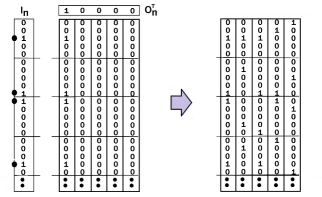
is an estimation of the weight matrix W(j) of the neural network as a linear associator with binary weights. Every synapse (matrix element) can update its weight independently and in parallel. This learning process is illustrated in Figure 1.

Figure 1 Showing a CMM learning input vector In associated with output vector On on the left. The CMM on the right shows the CMM after five associations IjOj

T

. Each column of the CMM represents a record. Each row represents a feature value for symbolic features or quantisation of feature values for continuous features and each set of rows (shown by the horizontal lines) represents the set of values or set of quantisations for a particular feature.

This process is identical to training the other feature values; the class is treated as an extra feature [30]. Figure 1 shows a trained CMM where each row is a feature or class value and each column represents a record. In this paper, we set only one bit in the vector Oj indicating the location of the record in the data set, the first record has the first bit set, the second record has the second bit set etc. Using a single set bit makes the length of Oj potentially large. However, exploiting a compact list representation [25] (more detail is provided in section 5) means we can compress the storage representation for single bit set vectors to a single index (set bit location), thus allowing AURA to be used for distributed processing with data sets of millions of records yet using a relatively small amount of memory.

2.2

Data

The AURA feature selector, classifier and predictor framework can handle symbolic, discrete numeric and continuous numeric features.

The raw data sets need pre-processing to allow them to be used in the binary AURA framework. Symbolic and numerical unordered features are enumerated and each separate token maps onto an integer (Token Integer) which identifies the bit to set within the vector. We refer to these features as symbolic henceforth. For example, a SEX_TYPE feature would map as (F 0) and (M 1). Any real-valued or ordered numeric features are quantised (mapped to discrete bins) [29], and each individual bin maps onto an integer which identifies the bit to set in the input vector. We refer to these features as continuous henceforth. Next, we describe the simple equi-width quantisation. We note that the Correlation-Based Feature Selector described in section 3.2 uses a different quantisation technique to determine the bin boundaries. However, once the boundaries are determined, the mapping to CMM rows is the same as described here.

To quantise continuous features, a range of input values for feature Fj map onto each bin. Each bin maps to a unique integer as in equation 2 to index the correct location for the feature in Ij. In this paper, the range of feature values mapping to each bin is equal to subdivide the feature range into b

equi-width bins across each feature.

(2)

In equation 2, offset(Fj) is a cumulative integer offset within the binary vector for each feature Fj and

offset(Fj+1) = offset(Fj) + nBins(Fj ) where nBins(Fj ) is the number of bins for feature Fj, is a many-to-one mapping and is a many-to-one-to-many-to-one mapping.

For each record in the data set For each feature

Calculate bin for feature value; Set bit in vector as in equation 2;

2.3

AURA Recall

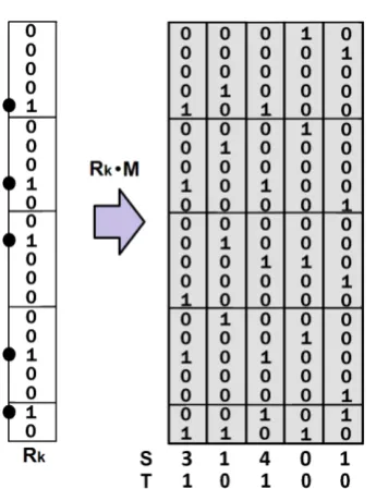
To recall the matches for a query record, we firstly produce a recall input vector Rk by quantising the target values for each feature to identify the bins (CMM rows) to activate as in equation 3. During recall, the presentation of recall input vector Rk elicits the recall of output vector Ok as vector Rk contains all of the addressing information necessary to access and retrieve vector Ok. Recall is effectively the dot product of the recall input vector Rk and CMM M, as in equation 3 and Figure 2.

Figure 2 Showing a CMM recall. Applying the recall input vector Rk to the CMM M retrieves a summed integer vector S with the match score for each CMM column. S is then thresholded to retrieve the matches. The threshold here is either Willshaw with value 3 retrieving all columns that sum to 3 or more or L-Max with value 2 to retrieve the 2 highest scoring columns.

If Rk appeared in the training set, we get an integer-valued vector S (the summed output vector), composed of the required output vector multiplied by a weight based on the dot product of the input vector with itself. If the recall input Rk is not from the original training set, then the system will recall the output Ok associated with the closest stored input to Rk, based on the dot product between the test and training inputs.

The AURA technique thresholds the summed output S to produce a binary output vector. For exact match, we use the Willshaw threshold [49]. This sets a bit in the thresholded output vector for every location in the summed output vector that has a value higher than or equal to a threshold value. The threshold varies according to the task. For partial matching, we use the L-Max threshold [9]. L-Max thresholding essentially retrieves at least L top matches. Our AURA software library automatically sets the threshold value to the highest integer value that will retrieve at least L matches.

Feature selection described in section 3 requires both exact matching using Willshaw thresholding and partial matching using L-Max thresholding.

3

Feature Selection

There are two fundamental approaches to feature selection [36][50]: (1) filters select the optimal set of features independently of the classifier/predictor algorithm while (2) wrappers select features which optimise classification/prediction using the algorithm. We examine the mapping of four filter

approaches to the binary AURA architecture. Filter approaches are more flexible than wrapper approaches as they are not directly coupled to the algorithm and are thus applicable to a wide variety of classification and prediction algorithms. They can then be used as stand-alone feature selectors for other classification or prediction algorithms exploiting the high speed and efficiency of the AURA techniques to perform feature selection which is a combinatorial problem. We also intend to integrate them with the AURA k-NN for classification and prediction in the unified AURA framework.

We examine a mutual information based approach (Mutual Information Feature Selection (MI)

greedily selected subsets of features, a revised Information Gain approach Gain Ratio (GR) detailed in section 3.3 and a feature dependence approach Chi-Square Feature selection(CS) detailed in section 3.4 which is univariate. Univariate filter approaches such as Mutual Information or Chi-square are quicker than multivariate as they do not need to evaluate all combinations of subsets of features. The advantage of a multivariate filter compared to a univariate filter lies in the fact that a univariate approach does not account for interactions between features. Multivariate techniques evaluate the worth of feature subsets by considering both the individual predictive ability of each feature and the degree of redundancy between the features in the set.

During training for the MI, CFS, GR and CS algorithms, the input vectors Ij represent the feature and class values in the data records and are associated with a unique output vector Oj. They all use an identical CMM and CMM training is an n-iteration process where n is the number of data records. This single CMM means that we can calculate and compare all four feature selectors using a single data representation. We note that the CFS as implemented by Hall [17] uses an entropy-based quantisation whereas we have used equi-width quantisation for the other feature selectors (MI, GR and CS ). We plan to investigate unifying the quantisation as a next step. For the purpose of our analysis in section 5, we assume that all feature selectors are using identical quantisation.

We assume that all records are to be used during feature selection.

3.1

Mutual Information Feature Selection

Wettscherek [48] described a mutual information feature selection algorithm. The mutual information between two features is ``the reduction in uncertainty concerning the possible values of one feature

that is obtained when the value of the other feature is determined' '[48]. We introduced an AURA

version of the MI feature selector in [34] and just provide a brief overview here.

For our feature selection, AURA excites the row in the CMM corresponding to feature value fi of feature Fj. This row is a binary vector (BV) and is represented by BVfi . A count of bits set on the row gives n(BVfi) from equation 4 and is achieved by thresholding the output vector Sk from equation 3 at Willshaw value 1. AURA also excites the row in the CMM corresponding to class value c where the binary vector is denoted BVc. Again, counting the number of bits set on the row as above gives n(BVc)

from equation 4.

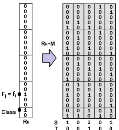
If both the feature value row and the class values row are excited then the summed output vector will have a two in the column of every record with a co-occurrence of fi with cj as shown in Figure 3. By thresholding the summed output vector at a threshold of two, we can find all co-occurrences. We represent this number of bits set in the vector by n(BVfi BVc) which is a count of the set bits when

BVc is logically ANDed with BVfi . The mutual information is given by equation 4 where rows(Fj) is the number of CMM rows for feature Fj and nClass is the number of classes:

(4)

We can follow the same process for real/discrete ordered numeric features in AURA. In this case, the mutual information is given by equation 5:

(5)

where bins(Fj) is the number of bins (effectively the number of rows) in the CMM for feature Fj , N is the number of records in the data set, BVbi is a binary vector (CMM row) for the quantisation bin mapped to by feature value fi, BVc is a binary vector with one bit set for each record in class c,

n(BVbi BVc) is a count of the set bits when BVc is logically ANDed with BVbi (as shown in Figure 3 and n(BVc) is the number of records in class c.

The MI feature selector assumes independence of features and scores each feature separately so it is the user's prerogative to determine the number of features to select. The major drawback of the MI feature selector along with similar information theoretic approaches, for example Information Gain, is that they are biased toward features with the largest number of distinct values as this splits the training records into nearly pure classes. Thus, a feature with a distinct value for each record has a maximal information score. The CFS and GR feature selectors described next make adaptations of information theoretic approaches to prevent this biasing.

3.2

Correlation-based Feature Subset Selection

Hall [17] proposed the Correlation-based Feature Subset Selection (CFS) which measures the strength of the correlation between pairs of features. CFS favours feature subsets that contain features that are highly correlated to the class but uncorrelated to each other to minimise feature redundancy. CFS is thus based on information theory measured using Information Gain. However, as noted in the previous section, Information Gain is biased toward features with the largest number of distinct values. Hence, Hall and Smith [20] used a modified Information Gain measure (Symmetrical Uncertainty) to estimate the correlation between features given in equation 6. Symmetrical Uncertainty effectively normalises the value in the range [0,1] where two features are completely independent if SU=0 and completely dependent if SU=1.

(6)

where the entropy of a feature Fj for all feature values fi is given as equation 7:

(7)

(8)

Any continuous features are discretised using Fayyad and Irani's entropy quantisation [12]. The bin boundaries are determined using Information Gain and these quantisation bins map the data into the AURA CMM as previously.

As noted previously, for feature selection, the class values and the associated records that take those class values are also trained into the CMM as extra rows (extra features) as shown in Figure 3. CFS has many similarities to MI through calculating the values in equations 6, 7 and 8 and through using the CMM as noted below.

In the AURA CFS, for each pair of features (Fj ,Gl) to be examined, the CMM is used to calculate Ent(Fj),

Ent(Gl) and Ent(Fj ·Gl) from equation 6. There are three parts to the calculation.

1. Ent(Fj)requires the count of data records for the particular value fi of feature Fj which is n(BVfi) in equation 4 for symbolic and class features and n(BVbi) in equation 5 for continuous features. Similarly, Ent(Gl) counts the number of records where feature Gl has value gk. 2. Ent(Fj ·Gl) requires the number of co-occurrences of a particular value fi of feature Fj with a

particular value gk of feature Gl as in equations 4 and 5 and Figure 3 except that CFS

calculates Ent(Fj ·Gl) between a feature and the class n(BVfi BVc) and n(BVbi BVc) as well as between pairs of features n(BVfi BVgk) and n(BVbi BVbk).

CFS determines the feature subsets to evaluate using forward search. Forward search works by greedily adding features to a subset of selected features until some termination condition is met whereby adding new features to the subset does not increase the discriminatory power of the subset above a pre-specified threshold value. The major drawback of CFS is that it cannot handle strongly interacting features [19].

3.3

Gain Ratio Feature Selection

Gain Ratio (GR) [43] is a new feature selector for the AURA framework. GR is a modified Information Gain technique and is used in the popular machine learning decision tree classifier C4.5 [43].

Information Gain is given in equation 9 for feature Fj and the class C. Hall and Smith [20] used a modified Information Gain measure in their CFS feature selector to prevent biasing toward features with the most values. GR is an alternative adaptation which considers the number of splits (number of values) of each feature when calculating the score for each feature using normalisation.

(9)

where Ent(Fj) is defined in equation 7 and Ent(Fj |C) is defined by equation 8. Then Gain Ratio is defined as equation 10:

(10)

where IntrinsicValue is given by equation 11:

(11)

and V is the number of feature values (n(Fj)) for symbolic features and number of quantisation bins

To implement GR using AURA, we train the CMM as described in section 2.1 using a suitable

quantisation for continuous features. This could be Fayyad and Irani's quantisation used in CFS or could be equi-width binning as described in section 2.2. We can then calculate Ent(Fj) and Ent(Fj| C) as per the CFS feature selector described in section 3.2 to allow us to calculate Gain(Fj, C). To calculate

IntrinsicValue(Fj) we need to calculate the number of records that have particular feature values. This is achieved by counting the number of set bits n(BVfi) in the binary vector (CMM row) for fi for

symbolic features or n(BVbi) in the binary vector for the quantisation bin bi for continuous features. We can store counts for the various feature values and classes as we proceed so there is no need to

calculate any count more than once. The main disadvantage of GR is that it tends to favour features with low Intrinsic Value rather than high gain by overcompensating toward a feature just because its intrinsic information is very low.

3.4

Chi-Square Algorithm

We now demonstrate how to implement a second new feature selector in the AURA framework. The Chi-Square (CS) [39] algorithm is a feature ranker like MI and GR rather than a feature selector; it scores the features but it is the user's prerogative to select which features to use. CS assesses the independence between a feature (Fj) and a class (C) and is sensitive to feature interactions with the class. Features are independent if CS is close to zero. Yang and Pedersen [51] and Forman [14] conducted evaluations of filter feature selectors and found that CS is among the most effective methods of feature selection for classification.

Chi-Square is defined as:

(12)

where b(Fj) is the number of bins (CMM rows) representing feature Fj, nClass is the number of classes,

w is the number of times fi and c co-occur, x is the number of times fi occurs without c, y is the number of times c occurs without fi, z is the number of times neither c nor fi occur. Thus, CS is predicated on counting occurrences and co-occurrences and, hence, has many commonalities with MI, CFS and GR.

 Figure 3 shows how to produce a binary output vector (BVfi BVc) for symbolic features or (BVbi BVc) for continuous features listing the co-occurrences of a feature value and a class value. It is then simply a case of counting the number of set bits (1s) in the thresholded binary vector T in Figure 3 to count w.

 To count x for symbolic features, we logically subtract (BVfi BVc) from the binary vector (BVfi) to produce a binary vector and count the set bits in the resulting vector. For continuous features, we subtract (BVbi BVc) from (BVbi) and count the set bits in the resulting binary vector.

 To count y for symbolic features, we can logically subtract (BVfi BVc) from (BVc) and count the set bits and likewise for continuous features we can subtract (BVbi BVc) from BVc and count the set bits.

 If we logically OR (BVfi) with (BVc), we get a binary vector representing (Fj=fi) (C=c) for symbolic features. For continuous features, we can logically OR (BVbi) with (BVc) to produce

(Fj=bin(fi)) (C=c). If we then logically invert this new binary vector, we retrieve a binary vector representing z and it is simply a case of counting the set bits to get the count for z.

4

Parallel and Distributed AURA

In distributed systems, data may be processed locally at each parallel compute node minimising communication overhead or globally across all overall data view [46].

4.1

Parallel

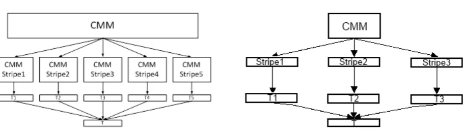
In Weeks et al. [47], we demonstrated a parallel search implementation of AURA. AURA can be subdivided across multiple processor cores within a single machine or spread across multiple connected compute nodes. This parallel processing entails striping the data across several parallel CMM subsections. The CMM is effectively subdivided vertically across the output vector as shown in

Figure 4. In the data, the number of features m is usually much less than the number of records N, hence, m << N. Therefore, we subdivide the data along the number of records N (column stripes) as shown in

Figure 4.

Figure 4 If a CMM contains large data it can be subdivided (striped) across a number of CMM stripes. In the left hand figure, the CMM is striped vertically (by time) and in the right hand figure the CMM is striped horizontally (be feature subsets). On the left, each CMM stripe produces a thresholded output vector Tn containing the top k matches (and their respective scores) for that stripe. All {Tn} are aggregated to form a single output vector T which is thresholded to list the top matches overall. On the right, each stripe outputs a summed output vector Sn. All Sn are summed to produce an overall summed output vector which is thresholded to list the top matches overall.

Splitting the data across multiple CMM stripes using columns means that the CMM can store data as separate rows within a single stripe. Each record is contained within a single stripe. Each separate CMM stripe outputs a thresholded vector from that CMM stripe.

If the number of features is large then it is possible to subdivide the CMMs further. The CMM is divided vertically by the records (column stripes) as before and then the column stripes are subdivided by the input features (row stripes). Dividing the CMM using the features (row stripes) makes assimilating the results more complex than assimilating the results for column stripes. Each row stripe produces a summed output vector containing column subtotals for those features within the stripe. The column subtotals need to be assimilated from all row stripes that hold data for that column. Thus, we sum these column subtotals to produce a column stripe vector C holding the overall sum for each column in that stripe. Row striping involves assimilating integer vectors of length c where c is the number of columns for the column subdivision (column stripe).

4.2

Distributed

distributed feature selection: maintaining a distributed data archive so that data does not have to be moved to a central repository and secondly, orchestrating the search process across the distributed data.

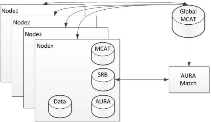
Figure 5 Distributed Data Management Architecture using a Pattern Match Controller accessing the Global Metadata Catalogue and Storage Resource Brokers on each processing node.

Our architecture for orchestrated search used a middleware stack (Pattern Match Controller [5] (PMC)) to farm search queries across distributed data resources. PMC allows a front-end service client to submit queries to all known data resources in a parallel, asynchronous manner, and to manage the processing and analysis of the data at the remote repositories. Forcing the pattern matching process to take place at the remote data repositories removes the costly requirement of moving large volumes of data during the search. An overview of the distributed AURA architecture is shown in Figure 5. The PMC uses a global Metadata Catalogue (global MCAT) that contains the locations of the data. In the implementation described in Austin et al. [5], the local data catalogue is provided by Storage Resource Broker [2] (SRB). SRB can manage distributed storage resources from large disk arrays to tape backup systems by mapping physical file locations to logical file handles referenced by PMC so PMC requires no knowledge of where the data resides. All nodes processing a query perform their search in parallel, searching all data held across the system as required. The PMC is also responsible for correlating the results and returning them.

Orchestrated search with minimal data movement can also be provided by the open source software project: Apache Hadoop [45]. Hadoop operates on the premise that moving computation is cheaper

than moving data [1]. Hadoop allows the distributed processing of large data sets across clusters of

commodity servers. It provides load balancing, is highly scalable and has a very high degree of fault tolerance. It is able to run on commodity hardware due to its ability to detect and handle failures at the application layer. When nodes fail with SRB, any search operations will not include results from these nodes. With Hadoop, there are multiple copies of the stored data so, if one server or node is unavailable, its data can be automatically replicated from a known good copy. If a compute node fails then Hadoop automatically re-balances the work load on the remaining nodes. There are two parts to Hadoop: MapReduce which assigns work to the nodes in a cluster and the Hadoop Distributed File System (HDFS) which is a distributed file system spanning all the nodes in the Hadoop cluster.

MapReduce jobs. This produces a very high aggregate bandwidth across the cluster. T applications specify the input/output locations and supply map and reduce functions via

implementations of appropriate interfaces and/or abstract-classes. The framework takes care of distributing the software/configuration, scheduling tasks, monitoring the tasks and re-executing any failed tasks.

HDFS links together the file systems on many local nodes to make them into one big file system. HDFS assumes nodes will fail, so it achieves reliability by replicating data across multiple nodes. Processing data in situ on local nodes is efficient compared to moving the data over the network to a single processing node. This local processing architecture of Hadoop has resulted in very good performance [44] on cheap computer clusters even with relatively slow network connections (such as 1 Gig Ethernet) [44]. Hence, Hadoop is ideal to underpin our distributed processing architecture.

5

Analysis

The key challenge for distributed feature selection is identifying the optimum method for distributing the search. Different data and applications will have different criteria that they wish to optimise. These could be optimising: communication overhead, processing speed, memory usage or combinations of these criteria. Hence, there is unlikely to be a single best technique for distribution.

However, Hadoop has demonstrated high performance for a wide variety of tasks [8]. It is aimed at batch processing tasks so is ideally suited to the task of feature selection where the feature selector is trained with the training data and feature selection is run once on a large batch of test data. In this paper, we focus on the implementation details of the four feature selectors using AURA with Hadoop. The capabilities of Hadoop have been demonstrated elsewhere [8] so we focus on describing how to map AURA CMMs to Hadoop to create an evaluation framework. Users will use this framework to select the best feature selector for their data and application using their own specific criteria.

Feature selection is a two part procedure. A training phase trains the data into the CMMs. A test phase then applies test data to the trained CMMs and correlates the results to produce feature selections. Each compute node holds a CMM that stores all local data. Data are trained into the CMM as described in section 2.1. During training, CMMs are not immutable as each association in equation 1 changes the underlying CMM so Hadoop MapReduce is not a suitable paradigm for CMM training. Hence, the CMMs are trained in a conventional fashion and uploaded to the Hadoop Distributed File System once trained. If the data stored in a node's CMM exceed the memory capacity of that node then the CMM is subdivided into stripes as described in section 4.1. The set of all CMM stripes at a node stores all data for that node. Every CMM stripe across the distributed system has to be coordinated so that record IDs (such as timestamps) are matched. If column 2 of one CMM stripe represents a time-stamp 10:00am on 31st May then column 2 in every associated row stripe must represent the identical time-stamp. When the results from different CMMs are unified then the columns from the various CMMs need to be aligned and hence must be identical time representations. The system is very flexible, we can access which nodes we require to access: all data or just a subset of data. The approach is a combination of the striping described above in section 4.1 and the CMM distribution described in section 4.2 with Hadoop orchestrating the search.

Each CMM stripe that receives a search request, executes the recall process described in section 2.3. This retrieves a set of candidate matches as a vector. The candidate matches are the set of stored patterns that are close to the query in the feature space. In Hadoop the processing is coordinated by MapReduce [45]. Hadoop schedules the MapReduce tasks independently of the problem being solved. There is one Map job for each input file. Therefore, we model feature selection as a series of

MapReduce jobs with each job representing one CMM stripe and the tasks are batches of file iterations (batch processing subsets of records) from the test data. The tasks are processed in parallel on

distributed nodes. Each CMM stripe is read into a job. The recall function for CMM stripes is written as a Map task. Each MapReduce job invokes multiple Map tasks, each task represents a batch of recalls for a subset of input records, the batches execute in parallel. The Hadoop Mapper keeps track of the output vector versus record ID pairs so we know which output vector is associated with which record. The Reduce tasks perform the integer output vector thresholding as described in section 2.3 and write the data back into the file associated with CMM stripe. Multiple feature selectors can be run in parallel, each executing as a series of MapReduce jobs. The CMMs for feature selection are immutable so subsequent iterations do not depend on the results (or changes) of the CMMs.

This whole MapReduce process has to be coordinated. If the MapReduce process is running at a single location then it can be coordinated as a Java class that initiates the individual jobs and then

coordinates the results from all jobs to produce the feature selection scores. If the processing is geographically distributed then it needs a more complete coordinator. This can be achieved using for example the UNIX curl command and a monitor process that determines when curl has collected new data. Alternatively, it can be achieved using a distributed stream processor such as Apache S4 (http://incubator.apache.org/s4/) or Twitter's STORM (https://github.com/nathanmarz/storm). Essentially, whichever tool is used this is a three part process: initiate the feature selection process at each of the distributed nodes; retrieve the results data from the distributed nodes; and, monitor when the results have been returned from all nodes and combine them into a single unified result. Each CMM stripe can return its results as

1. an integer vector Sk (unthrehsolded), 2. a thresholded vector Tk or

3. a list of the set bits in the thresholded vector.

The feature selection process produces a large set of output vectors from the CMM stripes; namely, all vectors necessary for all feature selectors. These results need to be amalgamated for each feature selector to produce the feature scores for that feature selector. Each feature selector will have a separate amalgamate program running at the coordinating node. This program uses the required vectors and set bit counts returned from AURA to produce the feature score as described in sections 3 and 5.1.

AURA has demonstrated superior training and recall speed compared to conventional indexing

approaches [25] such as hashing or inverted file lists which may be used for data indexing. AURA trains 20 times faster than an inverted file list and 16 times faster than a hashing algorithm. It is up to 24 times faster than the inverted file list for recall and up to 14 times faster than the hashing algorithm. AURA k-NN has demonstrated superior speed compared to conventional k-NN [27] and does not suffer the limitations of other k-NN optimisations such as the KD-tree which only scales to low dimensionality data sets [41]. We showed in [34] that using AURA speeds up the MI feature selector by over 100 times compared to a standard implementation of MI. Feature selection is a combinatorial problem so a fast and efficient platform will allow rapid analysis of large and high dimensional data sets.

5.1

Distributed Feature Selection

All four feature selection algorithms have been well documented elsewhere and their relative

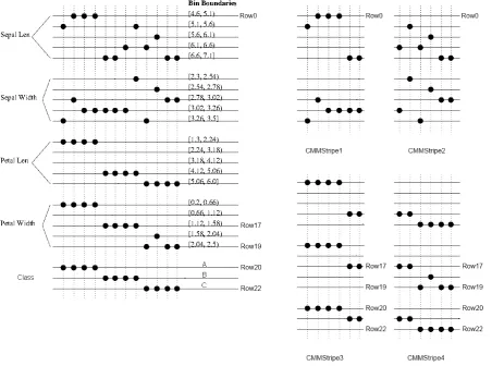
Figure 6 The 12 records from the iris data set, quantised and trained into a single AURA CMM (left) and subdivided across 4 stripes of the CMM (right). The letters in rows 20-22 indicate the class of the record: A=Iris-setosa, B=Iris-versicolor, C=Iris-virginica.

The feature selectors in section 3 have many commonalities when implemented in the unified AURA framework. We can demonstrate the commonalities by analysing 12 records from the Iris data set used in [34]. The data are illustrated in Figure 6 (left) when trained into the CMM. The 12 records have been trained into a CMM using the four features and the class. Each feature is continuous-valued and has been subdivided into five quantisation bins of equal width. Figure 6 (right) shows the same data divided into four CMM stripes (CMMStripe1,CMMStripe2, CMMStripe3 and CMMStripe4). The horizontal (row-based) striping means that the features sepal len and sepal width are in the top stripes and petal len , petal width and the class are in the bottom two stripes. The vertical (column-based) striping means that the first 6 data records are stored in the left two stripes and the other 6 records in the right two stripes. If the data were time-series or sequential, the column-based striping would form two time frames with the oldest data in the left two stripes and the newest data in the right two stripes. The input vectors are stored in a file for each CMM or CMM stripe. These files can then be batch processed in the Hadoop framework described. Within the evaluation, we consider how the data and CMMs would be accommodated in our Hadoop framework.

 MI, CFS, CS and GR can all use a single CMM representation for the data such as the CMM in Figure 6. This overall CMM is amenable to striping across the processing nodes to allow Hadoop processing in a similar fashion to

 MI, CFS, CS and GR all use BVfi (the binary vector where (Fj=fi)), BVbi (the binary vector representing the quantisation bin bin(fi)) and BVc (the binary vector representing all records that have a class label) so these only need to be extracted once and used in each feature selector as appropriate. For example in Figure 6, if we want all records where

1.12 petal width < 1.58 then we activate row 17 of the CMM using the input vector

00000000000000000100000 which will be one of the input vectors stored in the Hadoop input file for this CMM. We can then Willshaw threshold the integer output vector S at level 1 and retrieve the binary thresholded vector T with a bit set for every record where

1.12 petal width < 1.58, that is 000011110000 from Figure 6 (left). For the Hadoop

distributed version, we use input files that hold the vectors to be processed. The vectors are subdivided across CMM stripes so that only the data that are relevant to that CMM stripe are input. Activate row 17 of CMMStripe3 and CMMStripe4 using the input vector 00000100000 as these stripes hold the relevant data. CMMStripe3 will output 000011 and CMMStripe4 will output 110000 in Figure 6 (right). These can be concatenated to form a single vector

000011110000. For a fully distributed system, each CMM stripe outputs a list of the indices of the set bits for the data relevant to that stripe.

 MI, CFS and GR all require a count of the number of data records where a particular feature has a particular value n(Fj=fi) and a count of the number of records where the class has a particular label n(C=c). To count the number of records where 1.12 < 1.58, we retrieve the binary thresholded vector as above (000011110000) and count the number of set bits giving four records. For the Hadoop approach, we coordinate the retrieval as above, concatenate the lists to produce a single overall list of set bits and count the list length.  MI, CFS, CS and GR all use (BVfi BVc) and (BVbi BVv) for symbolic and continuous features

respectively. For example, we can find all records where 4.6 < 5.1 and the class is A

by activating rows 0 and 20 of the CMM using the input vector 10000000000000000000100 stored in the Hadoop input file for this CMM, thresholding at Willshaw level 2 to retrieve all records that match both inputs and retrieving the binary thresholded vector T, 011100000000 from Figure 6 (left). This takes more coordinating in the Hadoop framework as the data for the feature value may not be stored with the data for the class; they may be in different CMM stripes. Activate row 0 in CMMStripe1 and CMMStripe2 using input vector 1000000000. Activate row 20 in CMMStripe3 and CMMStripe4 using input vector 0000000000100. The coordinating program needs to correlate the sections of the vector for the feature value and correlate the sections of the vector for the class to form a single vector. CMMStripe1 needs to be added (summed) with the output integer vector of CMMStripe3 (011100+111100=122200) and CMMStripe2 needs to be added (summed) with the output integer vector of CMMStripe4

(000000+000000=000000). The summed vector can then be thresholded at 2 giving 011100 for Stripe1+Stripe3 and 000000 for Stripe2+Stripe4 in Figure 6 (right). These two thresholded output vectors are concatenated to produce 011100000000. If the thresholded vectors are stored as lists of indices then this is simply a task of finding the common indices between the two vectors.

 MI, CFS, CS and GR all also need a count of the conjunction, that is n(BVfi BVc) and

n(BVbi BVc) for symbolic and continuous features respectively. Hence, to count the number of records where petal width < 2.5 and the class is C, we retrieve the binary thresholded vector T (000000001011) and count the set bits giving 3 records. We coordinate the retrieval as above and, finally, count the number of set bits in the result.

Hence, rather than calculating these elements multiple times, we can take advantage of the

This requires the coordination of the vectors. To find (BVbi) (BVc), we combine the list of set bits for (BVbi) with the list of set bits for (BVc) and count the resulting list length. By calculating the common elements first, the remainder of the calculations can be performed for each feature selector using either this CMM and processing the algorithms in series or by generating multiple copies of the CMM and processing them in parallel if sufficient processing capacity is available.

For the Iris data set, there are n(BVbi) = 20 * BVbi calculations (20 row activations) and n(BVc) = 3 * BVc calculations. To calculate (BVbi BVc) requires n(BVbi) x n(BVc) = 20 x 3 =60 calculations. Hence, there are 83 common calculations (20+3+60) across all four feature selectors. CFS then needs to calculate (BVbi BVbk) which would require 19! calculations if every feature value was compared to every other. However, CFS uses greedy forward search so that the number of comparisons is minimised [17] to a worst case of (202-20)/2=190. We have already extracted all 20 * BVbi binary vectors so CFS needs 190 logical ANDs but no CMM accesses. We have saved a minimum of n(BVbi) = 20 CMM accesses to extract the 20 binary feature vectors BVbi and a maximum of 190 CMM accesses for worst case forward search. Manipulating the binary vectors can be performed at the coordinating node and in parallel as a Hadoop batch process. CS requires the logical OR vectors (BVbi BVc). Again, we already have all 20

BVbi binary vectors and all 3 BVc binary vectors so there are 20 x 3=60 logical ORs to perform. Thus, we have saved a minimum of n(BVbi) + n(BVc) = 23 CMM accesses and potentially 60 CMM accesses if all 60 OR operations were performed in the CMM. Thus MI requires 83 calculations, GR also requires 83, CFS requires 83 plus 190 and CS requires 83 plus 60. In total there are 83+83+83+190+83+60

calculations. We have reduced this to 83+190+60 and the 190+60 additional calculations (not

common) can use vectors already extracted so there is no need to access the CMM. We have saved

3 * 83=249 recalls from the CMM by finding common aspects, have removed a minimum of 20+23

further CMM recalls and have reduced the other calculations to logical operations on stored binary vectors. The minimum saving on CMM recalls is given by equation 13.

(13)

Once all of the binary vectors have been retrieved by the distributed Hadoop system, they need to be processed to calculate the feature scores using the various feature selectors. A coordinator program organises this and can be used to process in parallel. It takes the binary vectors stored in the files output from the Hadoop processing and uses these binary vectors to calculate the feature scores as per section 3. There is one feature score calculation process per feature selector (currently four feature selectors are described here). There is scope for subdividing the feature score calculations for each feature selector using parallel and distributed processing as appropriate to the location of the binary vectors required.

6

Conclusion

In this paper we have introduced a distributed processing framework for machine learning using the AURA neural network. There are currently four feature selectors available which may be used

ignored (masked off). Alternatively, the CMM can be retrained with only the required data if processing speed and memory usage at recall time are the primary concern.

The AURA neural architecture has demonstrated superior training and recall speed compared to conventional indexing approaches such as hashing or inverted file lists [25] and an AURA-based implementation of the MI feature selector was over 100 times faster than a standard implementation [34]. This allows rapid processing of feature selectors on large and high dimensional data sets. The user can then evaluate the feature sets chosen by the feature selectors against their own data to determine the best feature selector and the best set of features.

The technique is flexible and easily extended to other feature selection algorithms. We intend to introduce a ReliefR and an Odds Ratio feature selector among others. By implementing a range of feature selectors in a single framework, we can investigate ensemble feature selection where the results from a range of feature selectors are merged to generate a consensus overview of the best set of features to use.

We plan to use the feature selection framework that we have developed in this paper in conjunction with the AURA k-NN for traffic state [31][32][37], for traffic state prediction [33], for journey time prediction [30] and for condition monitoring [4].

7

References

[1] The Apache Software Foundation. Apache Hadoop Project [Online] (accessed 10/05/12) http://hadoop.apache.org/common/docs/r0.20.2/hdfs design.html, 2012.

[2] SDSC Storage Request Broker [Online] (accessed 10/05/12) http://www.sdsc.edu/srb/index.php/, 2012.

[3] J. Austin. Distributed associative memories for high speed symbolic reasoning. In R. Sun & F. Alexandre, editors, IJCAI '95 Working Notes of Workshop on Connectionist-Symbolic Integration: From Unified to Hybrid Approaches, pp. 87-93, Montreal, Quebec, August 1995.

[4] J. Austin, G. Brewer, T. Jackson & V. Hodge. AURA-Alert: The use of binary associative memories for condition monitoring applications. In Procs 7th I Conf. on Condition Monitoring and Machinery Failure Prevention Technologies, vol. 1, pp. 699-711, Stratford-upon-Avon, England, 2010.

[5] J. Austin, R. Davis, M. Fletcher, T. Jackson, M. Jessop, B. Liang & A. Pasley. Dame: Searching large data sets within a grid-enabled engineering application. Procs IEEE - Special Issue on Grid

Computing, 93(3):496-509, 2005.

[6] R. Beale & T. Jackson. Neural Computing: An Introduction. Institute of Physics Publishing, Bristol, U.K. and Philadelphia, PA, 1990.

[7] H. Bentz, M. Hagstroem & G. Palm. Selection of relevant features and examples in machine learning. Neural Networks, 2(4):289 - 293, 1997.

[8] D. Borthakur et al. Apache Hadoop goes Realtime at Facebook. In Procs 2011 I Conf. on Management of Data, SIGMOD '11, pp. 1071-1080, New York, NY, USA, 2011.

[9] D. Casasent & B. Telfer. High capacity pattern recognition associative processors. Neural

Networks, 5(4):251-261, 1992.

[10]M. Dash & H. Liu. Feature selection for classification. Intelligent Data Analysis, 1(3):131-156, 1997. [11]J. Dean and S. Ghemawat. MapReduce: Simplified Data Processing on Large Clusters, Comms of

the ACM, 51(1): 107-113, 2008.

[12]U. Fayyad & K. Irani. Multi-interval discretization of continuous-valued attributes for classification learning. In Procs I Joint Conf. on Artificial Intelligence, pp. 1022-1029, 1993.

[13]M. Fletcher, T. Jackson, M. Jessop, B. Liang & J. Austin. The signal data explorer: A high

[14]G. Forman. An extensive empirical study of feature selection metrics for text classification. J.

Mach. Learn. Res., 3:1289-1305, March 2003.

[15]I. Guyon & A. Elisseeff. An introduction to variable and feature selection. J. Mach. Learn. Res.,

3:1157-1182, March 2003.

[16]I. Guyon, J. Weston, S. Barnhill & V. Vapnik. Gene selection for cancer classification using support vector machines. Mach. Learn., 46(1):389-422, 2002.

[17]M. Hall. Correlation-based Feature Subset Selection for Machine Learning. PhD thesis, University of Waikato, Hamilton, New Zealand, 1998.

[18]M. Hall. Correlation-based feature selection for discrete and numeric class machine learning. In Procs 17th I Conf. on Machine Learning (ICML '00), pp. 359-366, 2000.

[19]M. Hall & G. Holmes. Benchmarking attribute selection techniques for discrete class data mining.

IEEE Trans. on Knowl. & Data Eng., 15(6):1437-1447, November 2003.

[20]M. Hall & L. Smith. Feature subset selection: a correlation based filter approach. In I Conf. on Neural Information Processing and Intelligent Information Systems, pp. 855-858, 1997.

[21]M. Hall & L. Smith. Practical feature subset selection for machine learning. In Procs of the 21st Australian Computer Science Conf., pp. 181-191, 1998.

[22]J. Han & M. Kamber. Data mining: concepts and techniques. The Morgan Kaufmann Series in Data Management Systems. Elsevier, 2006.

[23]V. Hodge. Integrating Information Retrieval and Neural Networks. PhD thesis, Department Of Computer Science, University of York, Heslington, York, UK, YO10 5DD, September 2001. [24]V. Hodge. Outlier and Anomaly Detection: A Survey of Outlier and Anomaly Detection Methods.

LAP LAMBERT Academic Publishing, 2011.

[25]V. Hodge & J. Austin. An Evaluation of Standard Retrieval Algorithms and a Binary Neural Approach. Neural Networks, 14(3), 2001.

[26]V. Hodge & J. Austin. A High Performance k-NN Approach using Binary Neural Networks. Neural

Networks, 17(3):441-458, 2004.

[27]V. Hodge & J. Austin. A Survey of Outlier Detection Methodologies. Artificial Intelligence Review, 22: 85-126, 2004.

[28]V. Hodge & J. Austin. A binary neural k-nearest neighbour technique. Knowl. Inf. Syst., 8(3):276-292, 2005.

[29]V. Hodge & J. Austin. Discretisation of Data in a Binary Neural k-Nearest Neighbour Algorithm.

Technical Report YCS-2012-473, Department of Computer Science, University of York, UK, 2012.

[30]V. Hodge, T. Jackson & J. Austin. A binary neural network framework for attribute selection and prediction. In 4th I Conf. on Neural Computation Theory and Applications - NCTA 2012, Barcelona, Spain, October 5-7 2012.

[31]V. Hodge, R. Krishnan, J. Austin & J. Polak. A computationally efficient method for on-line identification of traffic control intervention measures. In 42nd Annual UTSG Conf., University of Plymouth, UK, January 5-7 2010.

[32]V. Hodge, R. Krishnan, J. Austin & J. Polak. A computationally efficient method for online identification of traffic incidents and network equipment failures. In Transport Science and Technology Congress: TRANSTEC-2010, Delhi, India, April 4-7 2010.

[33]V. Hodge, R. Krishnan, J. Austin & J. Polak. Short-term traffic prediction using a binary neural network. In 43rd Annual UTSG Conf., Open University, Milton Keynes, UK, January 5-7 2011. [34]V. Hodge, S. O'Keefe & J. Austin. A binary neural decision table classifier. NeuroComputing,

69(16-18):1850-1859, 2006.

[35]I. Jolliffe. Principal Component Analysis. Springer-Verlag, New York, 2nd edition, 2002. [36]R. Kohavi & G. John. Wrappers for feature subset selection. Artif. Intell. J., Special Issue on

Relevance, 97(1-2):273-324, 1997.

[38]H. Liu, H. Motoda, R. Setiono & Z. Zhao. Feature selection: An ever evolving frontier in data mining. J. Mach. Learn. Res., pp. 4-13, 2010.

[39]H. Liu & R. Setiono. Chi2: Feature selection and discretization of numeric attributes. In Procs IEEE 7th I Conf. on Tools with Artificial Intelligence, pp. 338-391, 1995.

[40]H. Liu & R. Setiono. A Probabilistic Approach to Feature Selection - A Filter Solution. In Procs of 13th I Conf. on Machine Learning (ICML'96), pp. 319-327, 1996.

[41]A. McCallum, K. Nigam & L. Ungar. Efficient clustering of high-dimensional data sets with

application to reference matching. In Procs 6th ACM SIGKDD I Conf. on Knowledge Discovery & Data Mining (KDD-2000), 2000.

[42]J. Quinlan. Induction of decision trees. Mach. Learn., 1:81-106, 1986.

[43]J. Quinlan. C4.5 Programs for Machine Learning. Morgan Kaufmann, San Mateo, CA, 1992. [44]N. Rutman. Map/reduce on lustre, (white paper). Technical report, Xyratex Technology Limited,

Havant, Hampshire, UK, 2011.

[45]K. Shvachko, K. Hairong, S. Radia & R. Chansler. The Hadoop distributed file store system. In Procs IEEE 26th Symp. on Mass Storage Systems and Technologies (MSST), 28 June, 2010.

[46]P. Varshney. Multisensor data fusion. Electronics Comm. Engineering Journal, 9(6):245-253, 1997. [47]M. Weeks, V. Hodge & J. Austin. A hardware accelerated novel IR system. In Procs 10th Euromicro

Workshop (PDP-2002), Gran Canaria, Jan. 9-11. IEEE Computer Society, CA, 2002.

[48]D. Wettscherek. A study of distance-based machine learning algorithms. PhD thesis, Department of Computer Science, Oregon State University, Corvallis, USA, 1994.

[49]D. Willshaw, O. Buneman & H. Longuet-Higgins. Non-holographic associative memory. Nature, 222:960-962, 1969.

[50]I.H. Witten & E. Frank. Data Mining: practical machine learning tools and techniques with Java

implementations. Morgan Kaufmann, 2000.