A system identification based approach for pulsed eddy current non-destructive evaluation

promoting access to White Rose research papers

Universities of Leeds, Sheffield and York

http://eprints.whiterose.ac.uk/

This is an author produced version of a paper published in

Measurement

Science and Technology.

White Rose Research Online URL for this paper:

http://eprints.whiterose.ac.uk/2665/

Published paper

Lang, Z.Q., Agurto, A., Tian, G.Y. and Sophian, A. (2007)

A system identification

based approach for pulsed eddy current non-destructive evaluation

,

A

S

YSTEM IDENTIFICATION BASED APPROACH FOR PULSED

EDDY CURRENT NON-DESTRUCTIVE EVALUATION

Z Q Lang*, A Agurto#, G Y Tian#, and A Sophian#

*Department of Automatic Control and Systems Engineering The University of Sheffield, UK

Email:[email protected]

#

Department of Electrical and Electronic Engineering The University of Newcastle, UK

Email:[email protected]

Abstract

This paper is concerned with the development of a new system identification based approach for pulsed eddy current non-destructive evaluation and the use of the new approach in experimental studies to verify its effectiveness and demonstrate its potential in engineering applications.

1. Introduction

Non-destructive Evaluation (NDE) techniques have been widely used in many engineering areas [1]. Particularly, eddy current NDE has been used for the inspection of defects in metals for decades. An effective NDE system should be able to detect whether a defect has appeared in a structure, classify a detected defect into a particular category, and even quantify the defect details such as location, size and orientation.

structures can produce the changes of this differential signal, the differential signal based NDE methods have been widely used in NDE community to detect and categorise defects in structures.

In the present study, the difficulty with an effective interpretation of the response signal in pulsed eddy current NDE is addressed from a totally different but novel perspective. Instead of analysing the differential signal as conducted in almost all available techniques, we propose to apply the system identification approach to establish a transfer function model for inspected structures from the measured eddy current sensor response to the pulsed coil excitation, and to use the model parameters to reflect the changes of the structural characteristics due to, e.g., flaws and conductivity and dimensional changes. Compared with the widely used differential signal, the structural model parameters can not only provide a more compact description for the structural characteristics but can also better reveal the real mechanism which dominates the structural dynamic behaviours including the eddy current sensor response to a pulsed coil excitation. The proposed system identification method has potentials for not only local but global defect identification such as defect sizing and location, which can be extended for bridging the gap of structural health monitoring and NDE.

In addition to the use of the system identification approach to determine the characteristics of structure integrity in terms of the parameters of an identified transfer function model, in this paper, we also propose to use Fisher Discriminant Analysis (FDA) and Fisher Discriminant functions for defect pattern classification [5]; FDA is not only a powerful dimensionality reduction technique for feature extraction but also takes into account the information between defect classes when determining a lower-dimensional representation. After the identified transfer function model for an inspected structure has been obtained, FDA is applied to the identified transfer function model parameters to reduce the dimension of the parameter vector used to represent the structure characteristics so as to minimise the rate of misclassification, and then Fisher Discriminant Functions for all available defect classes are used to perform defect pattern classification.

In order to evaluate the performance of this proposed new NDE approach, the approach is applied to analyse experimental test results on two sets of aluminium specimens, each set consisting of specimen of three different defects. The results of the experimental data analyses sufficiently verify the effectiveness of the new technique, and demonstrate that the new system identification based pulsed eddy current NDE approach has great potential in engineering applications.

2 System identification

For example, consider the case where the relationship between the input and output of a system or structure can be described by a second order differential equation as follows

)

(

)

(

)

(

)

(

)

(

2 1 2 1 2 2

t

u

b

dt

t

du

b

t

y

a

dt

t

dy

a

dt

t

y

d

₊

₊

₌

₊

(1)

where

y

(t

)

and

u

(t

)

represent the output and input of the system or structure respectively, and

a

₁,

a

₂,

b

₁, and

b

₂ are the parameters of the differential equation model, which define the system or structure’s dynamic characteristics. In the frequency domain, the differential equation model (1) can be written as

)

(

)

(

)

(

)

(

)

(

_{1 2 1 2}

2

s

u

b

s

su

b

s

y

a

s

sy

a

s

y

s

+

+

=

+

(2)

to yield an transfer function based input output model description as

2 1 2 2 1

)

(

)

(

)

(

a

s

a

s

b

s

b

s

H

s

u

s

y

+

+

+

=

=

(3)

In Equations (2) and (3),

s

is the Laplace operator,

y

(s

)

and

u

(s

)

are the Laplace transform of

y

(t

)

and

u

(t

)

respectively, and

H

(s

)

is the transfer function of system (1).

Given the input

u

(t

)

and output response

y

(t

)

of system (1), such as, e.g., a pulsed input and its corresponding response, the parameters of the system can be determined using a system identification technique known as Prediction error method [7]. The idea of this method is to use an optimisation method to solve the following problem:

dt

t

y

t

y

T t b b a

a

∫

=0

−

2 ˆ , ˆ , ˆ , ˆ

))

(

)

(

ˆ

(

MIN

2 1 2 1 (4)

where T is the time period over which the response signal y(t) to the input u(t) is measured,

2 1 2 1

,

ˆ

,

ˆ

,

ˆ

ˆ

a

b

b

a

represent the estimates of the system parameters, and

y

ˆ

(

t

)

is the solution to the differential equation

)

(

ˆ

)

(

ˆ

)

(

ˆ

)

(

ˆ

)

(

2 1 2 1 2 2

t

u

b

dt

t

du

b

t

y

a

dt

t

dy

a

dt

t

y

d

₊

₊

₌

₊

(5)

Denote the solution to the optimisation problem (4) as

a

ˆ

₁*

,

a

ˆ

*₂

,

b

ˆ

₁*

,

b

ˆ

₂*. Then the estimated differential equation model

)

(

ˆ

)

(

ˆ

)

(

ˆ

)

(

ˆ

)

(

* 2 * 1 * 2 * 1 2 2

t

u

b

dt

t

du

b

t

y

a

dt

t

dy

a

dt

t

y

d

₊

₊

₌

₊

(6)

* 2 * 1 2

* 2 * 1 *

ˆ

ˆ

ˆ

ˆ

)

(

ˆ

a

s

a

s

b

s

b

s

H

+

+

+

=

(7)

can be used to represent the system or structure’s dynamic behaviours, and the estimated

model parameters

a

ˆ

₁*

,

a

ˆ

₂*

,

b

ˆ

₁*

,

b

ˆ

₂* or functions of them can be used to represent different features of the characteristics of the system or structure described by Equation (1).

3 Fisher Discriminant Analysis and Fisher Discriminant functions [5]

Fisher discriminant analysis (FDA) and fisher discriminant functions are the methods associated with pattern classification. The typical pattern classification system assigns an observation vector to one of several classes via three steps which are feature extraction, discriminant analysis, and maximum selection. The feature extraction step is to increase the robustness of the pattern classification system by reducing the dimensionality of the observation vector in a way that retains most of the information discriminating amongst the different classes. Using the information in the reduced-dimensional space, the discriminant analysis evaluates, for each class, the value of a discriminant function which is defined as the posteriori probability of an observation vector belonging to a class, and quantifies the relationship between the observation vector and the class. Finally the step of maximum selection assigns the observation vector to a class for which the discriminant analysis result reaches the maximum.

FDA is a very effective feature extraction/dimensionality reduction technique, which takes into account the information between the classes and has advantages over other methods such as Principal Component Analysis (PCA) for fault diagnosis. Fisher Discriminant functions are a specific discriminant function associated with the results of FAD for discriminant analysis.

Define n as the number of observations in a training data set, m as the number of measurement variables for each observation, p as the total number of classes the observations belong to in the training data set, and nj as the number of observations in the

jth class, j=1,…,p. Represent the vector of measurement variables for the ith observation as

i

x, i=1,…,n.

The FDA based feature extraction is conducted based on two (m×m) matrices which are within-class-scatter matrix S_w and between-class-scatter matrix S_b generated from a training data set as follows.

∑

=

= p

j j

w S

S

1

(8)

(

)(

)

T j i j i x

j x x x x

S

j i

− −

=

∑

∈χ

(9)

j

χ is defined as the set of vectors x_i which belong to the class j, and

∑

∈

=

j i

x i j

j x

n x

χ

1

(

)(

)

T

j j p

j j

b n x x x x

S =

∑

− −

=1

(10)

where

∑

=

= n

i i x n x

1

1 .

From S_w and S_b evaluated from (8)-(10), at most p-1 nonzero eigenvectors w_k, k=1,…,p-1,

of the generalized eigenvalue problem

k w k k

bw S w

S =λ , k=1,...,p−1 (11)

can be determined using any software package that does matrix manipulations such as MATLAB. In (11), λ_k denotes the eigenvalue associated with w_k, which indicates the

degree of overall separability among the classes by projecting the data onto w_k.

Let

] , , ,

[ _{1 2 −1}

= p

p w w w

W L (12)

Then, given a new observation data vector x, the FDA is conducted by performing the linear transformation

x W

z T

p

= (13)

to transform the data x in m-dimensional space to the data z in (p-1)-dimensional space for the purpose of a more effective discriminant analysis.

More specifically speaking, FDA first computes the matrix W_p using equations (8)-(12)

such that training data x₁,L,x_n from p classes are optimally separated when projected into the p-1 dimensional space as z_i =W_pTx_i,

i

=

1

,...,

n

. Then, for any new observation data x,

the same linear transformation defined by the matrix Wp is applied as given by (13) to

produce a low dimensional observation z. The low dimensional observation z can then be used by p Fisher discriminant functions, which quantify the relationship between the new data represented by x or z with each of the available p classes, to perform discriminant analysis.

)] 1

1 ln[det( 2 1 ) ln( ) ( ) 1

1 ( ) ( 2 1 )

( 1 _pT _{j p}

j j

j p

j T p j T j

j W SW

n p

z z W S W n z z z

g

− −

+ − −

− −

= −

j=1,…,p (14)

where T _j

p

j W x

z = , and p_j is the a priori probability for class j, j=1,…,p.

In the end, the new observation x or z will be assigned to class j* such that )

( max )

(

} ,..., 1 {

* z g z

g _j

p j

j = _∈ (15)

following the principle of maximum selection in the last step of pattern classification.

4. A system identification based approach for pulsed eddy current NDE

As an experimental data based modelling approach, the system identification has been widely used in various science and engineering areas for establishing mathematical models for systems and/or structures in order to understand system/structure’s behaviours, to predict system/structures’ responses to different inputs, and even to perform automatic control of system/structures based on an established mathematical model description. Pattern classification using PDA and Fisher Discriminant functions is a well established and very effective technique for fault diagnosis given observation vectors consisting of measurements which reflect the working conditions of systems or structures under inspection.

Eddy current NDE system consisting of an excitation coil, metal sample and magnetic detector (coil or magnetic sensors) can be considered as a system [8]. Considering the capability and advantage of the system identification in revealing the characteristics of systems and structures and in dealing with noises and measurement errors, and the effectiveness of PDA and Fisher Discriminant functions in conducting pattern classification, a system identification based approach for pulsed eddy current NDE is proposed in the present study. The basic procedure of this approach is:

(1) Use a system identification technique to establish a transfer function model for the inspected systems or structures from a pulsed coil excitation and the measured eddy current sensor response, and use the estimated parameters for the transfer function model to reflect the system or structure’s characteristics.

(2) Use FDA to extract the significant features of inspected systems or structures from the estimated transfer function model parameters, and assign the inspected system or structure into a class representing a particular working or defective condition using the procedures of Fisher discriminant analysis and maximum selection

To implement this approach, a training process needs first to be conducted. This involves:

(b) Establishing a transfer function model from each excitation and corresponding response.

(c) Performing the operations in equations (8)-(11), where

x

_i represents the transfer function parameter estimates obtained from the ith excitation and corresponding response, i=1,…,n, to determine the linear transformation matrix

W

_p.

Matrix

W

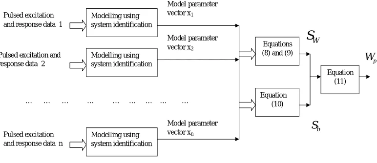
_p obtained in step (c) above will then be used to perform Fisher discriminant analysis on new data sets.

Assume that in total n sets of excitation and response data collected for NDE tests on specimens representing p different defective and/or working conditions are available for the training process, and there are

n

_j sets of excitation and response data representing the jth (j=1,…,p ) defective and/or working condition in the training data. Then, by denoting the transfer function model parameters estimated from the ith set of excitation and response data as

[

i im

]

i

x

x

x

=

₁

,

L

,

i=1,…,n

where m represents the number of the model parameters, equations (8)-(11) can be used to determine the result from the training process that is the linear transformation matrix

] , , ,

[ 1 2 −1

= p

p w w w

W L . Figure 1 illustrates this training process and shows schematically

how the FDA linear transformation matrix W_p can be obtained from the pulsed coil

excitation based tests on the specimens representing p different defective and/or working conditions.

Modelling using system identification

Modelling using system identification

Modelling using system identification Pulsed excitation

and response data 1

Pulsed excitation and response data 2

Pulsed excitation and response data n

… … … … … … … … … Model parameter vector x1

Model parameter vector x2

Model parameter vector xn

Equations (8) and (9)

Equation (10)

W

S

b S

Equation (11)

p

[image:8.612.126.512.448.615.2]

W

Figure 1 The generation of FDA linear transformation matrix from training data

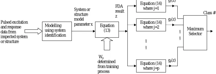
NDE can be applied on-line as shown in Figure 2 to determine the defective or working condition of an inspected system or structure from the system or structure’s response to a pulse excitation. The pulsed excitation and the corresponding eddy current sensor response measured from the system or structure are first used to determine a transfer function model of the system or structure. Then the FDA is applied to extract the features of the system or structure from the estimated transfer model parameters. Finally, the maximum selection process is applied to the results evaluated from p Fisher discriminative functions, and the class of defective or working condition that corresponds to the maximum Fisher discriminative function value is assigned to the system or structure under inspection.

It is well-known that the defective or working conditions of systems or structures are essentially determined by the systems or structural integrity characteristics. For example, in metal structures, these conditions are determined by microstructures, surface form and roughness, natural crack, residual stress beyond tradition discontinuity crack, and corrosion etc many factors. Conventional NDE techniques depend directly on sensor measurement signals to perform analysis and to conduct pattern classification. However, any direct measurement from NDE oriented tests can only reflect these material characteristics indirectly, and the measurement results also unavoidably prone to the effects of measurement errors and noises. For example, although the distinctive advantage of pulsed eddy current NDE is that the measured signal covers a wide range of spectrum so as to be able to reflect defects of different depths, the unavoidable high frequency noise effects on the measured wideband signals may not be negligible and may consequently impair the NDE results.

In order to solve these problems with conventional NDE techniques especially the problems caused by noises, many advanced signal processing based techniques have recently been proposed by researchers. In contrast with conventional NDE techniques and these recent advanced signal processing based methods, the new system identification based pulsed eddy current NDE approach does not perform the NDE analysis directly using eddy current sensor measurements. Instead, the new approach conduct the NDE analysis based on the features extracted from the parameters of an identified transfer function model of the inspected system or structure via a FDA operation. Because the system or structure’s dynamic behaviours are uniquely defined by the model parameters, these parameters should be more directly related to the system or structure’s characteristics than direct sensor measurements, and the features extracted from the estimated model parameters via FDA should consequently provide a much clearer picture relating to the physical properties of

Modelling using system identification Pulsed excitation

and response data from inspected system or structure

System or structure model

parameter x _Equation (13)

Equation (14) where j=1 Equation (14)

where j=2

M M

Equation (14) where j=p FDA

result z

Maximum Selector

M M

Class #

Wp

determined from training process

g1(z)

g2(z)

[image:9.612.133.491.391.514.2]

gp(z)

concern by field engineers. In addition, because most system identification methods are capable to deal with noise and measurement errors, the effects of noise and measurement errors on the analysis results can also be significantly reduced.

In order to evaluate the performance of the proposed novel NDE approach, the analysis of the experimental data collected from eddy current NDE tests on two sets of specimens under different defective conditions has been conducted. Details of the experimental setup, the specimens that were tested, and the analysis results are given in the following sections.

5 Experimental setup, tested specimens, and experiments on the

specimens

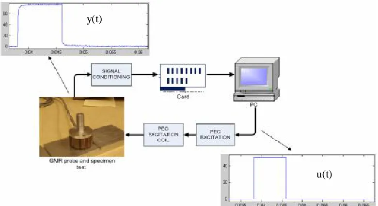
Figure 3 illustrates schematically the experimental setup for conducting the NDE tests in the present study. A pulse signal u(t) is generated by a PC to excite the coil and generate pulse eddy current inside a tested specimen. A GMR (Giant Magnetoresistive) probe placed on top of the specimen receives the EM (electromagnetic field transient) signal and produces the sensor response y(t) to the pulsed excitation.

[image:10.612.110.500.439.652.2]

Two sets of aluminium specimens have been tested. In the first specimen set, there are three specimens belonging to three defective classes, which are no defect, 20mm surface slot defect, and 40mm surface slot defect. In the second specimen set, there are in total 23 specimens: 12 specimens belong to the defective class of metal loss to the extent of between 2 and 10mm; 5 specimens belong to the defective class of surface slot to the extent of 2, 4, 6, 8 mm; and 6 specimens belong to the defective class of sub-surface slot to the extent of 2, 4, 6, 8 mm. The sample detail can be found in [1].

Figure 3 The experimental setup for the conducted NDE tests y(t)

y(t)

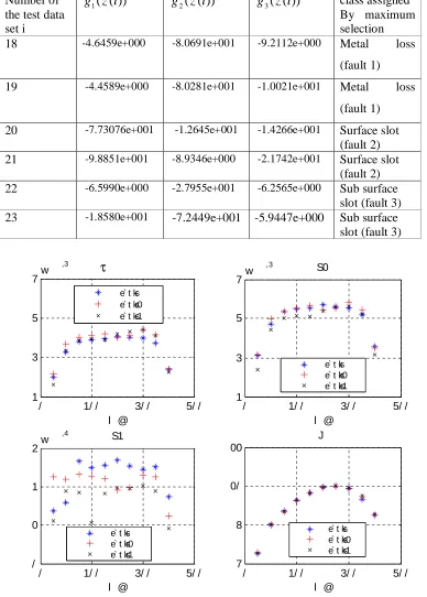
In the experimental tests on the first set of specimens, all specimens were excited by a pulsed signal u(t) ten times with a pulse magnitude being 50mA, 100mA, 150mA, 200mA, 250mA, 300mA, 350mA, 400mA, 450mA, and 500mA, respectively. These excitations and their corresponding responses were sampled at the frequency 100KHz to produce, in total, 30 sets of excitation and response (input and output) data. Only signals obtained over the excitation range between 200mA and 400mA were used for analysis due to the linear relationships between excitations and responses over this range as indicated by the estimated value for K shown in Figure 4. Thus, in total, 15 sets of input output data are available. Of the 15 sets of input output data, three from defect free specimen (Data sets 1,2,3), three from 20 mm surface slot defect specimen (Data sets 4,5,6), and three from 40 mm surface slot defect specimen (Data sets 7,8,9) were used as the training data sets, and the rest (Data sets 10-11 from defect free specimen, Data sets 12-13 from 20mm surface slot defect specimen, and Data sets 14-15 from 40 mm surface slot defect specimen) were used as new data to evaluate the performance of the proposed approach in classifying the specimen conditions represented by these data into corresponding classes.

The experimental tests on the second set of specimens were conducted such that all the 23 specimens were excited once by the pulsed signal u(t) with the magnitude of 500mA. The excitations and corresponding responses were sampled at the frequency of 1MHz to produce, in total, 23 sets of input and output data. Of the 23 sets of input output data, ten from metal loss defect specimens (Data sets 1-10), three from surface slot defect specimens(Data sets 11-13), and four from sub-surface slot defect specimen (Data sets 14-17) were used as the training data sets, and the rest, which are two from metal loss (Data sets 18,19), two from surface slot (Data sets 20,21), and two from sub-surface slot (Data sets 22, 23) were used as new data to evaluate the performance of the proposed approach in classifying the specimen conditions represented by these data into corresponding classes.

6.

The results of experimental data analysis

6.1

Analysis results for the first set of aluminium specimens

For the first set of specimens, after some initial trios, the transfer function model of the form

)

1

)(

1

(

)

1

(

)

(

2

1

+

+

+

=

s

T

s

T

s

K

s

H

τ

(16)

was used for the system identification based modelling process. The transfer function in (16) can be further written as

)

/

1

(

]

/

)

[(

)

/

(

)

/

(

)

(

2 1 2

1 2 1 2

2 1 2

1

T

T

s

T

T

T

T

s

T

T

K

s

T

T

K

s

H

+

+

+

+

=

τ

(17)

indicating that the transfer function model is the same as that in (3) with

2 1 1

K

/

T

T

b

=

τ

/

T

T

K

]

/

)

[(

_{1 2 1 2}

1

T

T

T

T

a

=

+

)

/

1

(

_{1 2}

2

T

T

a

=

Figure 4 shows the thirty sets of

K

,

τ

,

T

₁

,

T

₂ estimated using the system identification approach from the data collected from the ten NDE tests on the first set of three specimens. From the nine sets of the estimated

K

,

τ

,

T

₁

,

T

₂ for training, a

(

4

×

2

)

dimensional FDA linear transformation matrix is worked out using the procedure described in Section 3 as

]

[ _{1 2}

3 w w

W

W_p = = (18)

where

T

w

1

=

[

-

1.0861e

-

005,

6.7705e

-

006,

-

2.6161e

-

006,

3.0493e

-

002

]

T

w

₂

=

[

-

2.7970e

-

005,

3.8760e

-

006,

1.1709e

-

005,

1.9953e

-

002

]

Denote the estimated

K

,

τ

,

T

₁

,

T

₂ from the ith of the fifteen sets of input output data used for analysis as

K

ˆ

(

i

),

τ

ˆ

(

i

),

T

ˆ

₁

(

i

),

T

ˆ

₂

(

i

)

, i=1,…,15. Then, using the results for training,

)

(

ˆ

),

(

ˆ

),

(

ˆ

),

(

ˆ

2 1

i

T

i

T

i

i

K

τ

,i=1,…,9, nine (p-1)=(3-1)=2 dimensional FDA vectors are generated

as





























=

)

(

ˆ

)

(

ˆ

)

(

ˆ

)

(

ˆ

)

(

2 1 3

i

T

i

T

i

i

K

W

i

z

T

τ

i=1,…,9 (19)

Figure 5 shows the 9 FDA vectors and indicates very clearly that the FDA analysis separates the 9 vectors into three different regions (

z

(

1

)

−

z

(

3

)

in region I,

z

(

4

)

−

z

(

6

)

in region II, and

z

(

7

)

−

z

(

9

)

in region III) in the two dimensional FDA space, each representing one class of defective condition.

Of the 15 sets of

K

,

τ

,

T

₁

,

T

₂ estimated, nine are used for training as described above; the remaining six, which are

K

ˆ

(

i

),

τ

ˆ

(

i

),

T

ˆ

1

(

i

),

T

ˆ

2

(

i

)

, i=10,…,15, are used as new data to

evaluate the performance of the proposed new NDE approach. The mappings of these six sets of new data into the two dimensional FDA space are given by





























=

)

(

ˆ

)

(

ˆ

)

(

ˆ

)

(

ˆ

)

(

2 1 3

i

T

i

T

i

i

K

W

i

z

T

τ

The

z

(i

)

, i=10,…,15, thus obtained are also shown in Figure 5, indicating that every set of new data has been correctly placed into the region which represents its corresponding defective class. This observation is in fact consistent with the results from the fisher discriminant functions (14) based maximum selection, which are obtained as follows.

Evaluate

)]

1

1

ln[det(

2

1

)

ln(

)

)

(

(

)

1

1

(

)

)

(

(

2

1

))

(

(

_{3 3} 1

W

₃

S

W

₃

n

p

z

i

z

W

S

W

n

z

i

z

i

z

g

T _j

j j

j j

T

j T j

j

=

−

−

₋

−

+

−

₋

−

(21)

for i=10,…,15 and j=1,2,3, where

p

_j

=

1

/

3

, j=1,2,3 and

z

_j

,

n

_j,

S

_j, j=1,2,3, are determined from the 9 training data sets of

K

ˆ

(

i

),

τ

ˆ

(

i

),

T

ˆ

₁

(

i

),

T

ˆ

₂

(

i

)

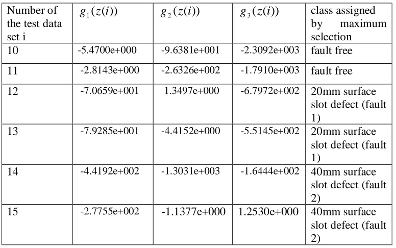
, i=1,…,9. The results are shown in Table 1.

[image:13.612.109.524.152.222.2]

Clearly the maximum selection procedure assigns the new data into correct classes. The analysis on the experimental data from the first set of specimens therefore verifies the effectiveness of the proposed new NDE approach.

Table 1 The results obtained from Fisher Discriminant Function based maximum selection for the first set of specimens

Number of the test data set i

))

(

(

1

z

i

g

g

₂

(

z

(

i

))

g

₃

(

z

(

i

))

class assigned

by maximum

selection

10 -5.4700e+000 -9.6381e+001 -2.3092e+003 fault free

11 -2.8143e+000 -2.6326e+002 -1.7910e+003 fault free

12 -7.0659e+001 1.3497e+000 -6.7972e+002 20mm surface

slot defect (fault 1)

13 -7.9285e+001 -4.4152e+000 -5.5145e+002 20mm surface

slot defect (fault 1)

14 -4.4192e+002 -1.3031e+003 -1.6444e+002 40mm surface

slot defect (fault 2)

15 -2.7755e+002 -1.1377e+000 1.2530e+000 40mm surface

[image:13.612.124.512.441.684.2]

6.2

Analysis results for the second set of aluminium specimens

For the second set of specimens, again after some initial trios, the transfer function model of the form 2

)

(

2

1

~

)

(

s

T

s

T

K

s

H

ω ω

ξ

+

+

=

(22)

was used for the system identification based modelling process. Rewriting (22) as

2 2 2

)

/

1

(

)

/

2

(

)

/

~

(

)

(

ω ω ω

ξ

T

s

T

s

T

K

s

H

+

+

=

(23)

indicates that the transfer function model is the same as that in (3) with

0

1

=

b

2 2

/

~

ω

T

K

b

=

)

/

2

(

1

ξ

T

ω

a

=

2 2

(

1

/

T

ω

)

a

=

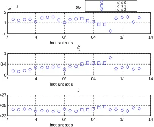
Figure 6 shows the 23 sets of

T

_ω

,

ξ

,

K

~

estimated using the system identification approach from the data collected from the NDE tests on the second set of 23 specimens. From the 17

sets of the estimated

T

_ω

,

ξ

,

K

~

for training, a

(

3

×

2

)

dimensional FDA linear transformation matrix is worked out using the procedure described in Section 3 as

] ~ , ~ [ ~ ~ 2 1

3 w w

W

W_p = = (24)

where

]

000

+

1.0000e

-004,

-3e

003,-2.564

-7.0211e

-[

~

1

=

w

]

000

+

1.0000e

003,

-1.9129e

004,

-3.5674e

[

~

2

=

w

Denote the estimated

T

_ω

,

ξ

,

K

~

from the ith set of training data as

T

ˆ

_ω

(

i

),

ξ

ˆ

(

i

),

K

~

ˆ

(

i

)

,

i=1,…,17. Then, using

T

ˆ

_ω

(

i

),

ξ

ˆ

(

i

),

K

~

ˆ

(

i

)

, i=1,…,17, seventeen (p-1)=(3-1)=2 dimensional FDA vectors are generated as





















=

)

(

ˆ

~

)

(

ˆ

)

(

ˆ

~

)

(

~

3

i

K

i

i

T

W

i

z

T

ξ

ω

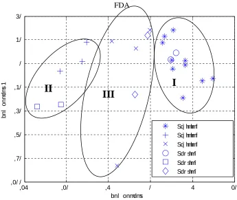
Figure 7 shows the 17 FDA vectors and indicates again very clearly that the FDA analysis separates the 17 vectors into three different regions (

~

z

(

11

)

−

~

z

(

13

)

in region II,

)

17

(

~

)

14

(

~

_z

₋

_z

_{in region III, and}

_z

~

₍

₁

₎

₋

~

_z

₍

₁₀

₎

_{in region I) in the two dimensional FDA}

space, each representing one class of defective condition.

Of the 23 sets of

T

_ω

,

ξ

,

K

~

estimated, seventeen are used for training as described above; the

remaining six, which are

T

ˆ

_ω

(

i

),

ξ

ˆ

(

i

),

K

ˆ~

(

i

)

, i=18,…,23, are used as new data to evaluate the performance of the proposed new NDE approach. The mappings of these six sets of new data into the two dimensional FDA space are given by





















=

)

(

ˆ

~

)

(

ˆ

)

(

ˆ

~

)

(

~

3

i

K

i

i

T

W

i

z

T

ξ

ω

, i=18,…,23. (26)

As seen from Figure 7, putting

~

z

(

i

)

, i=18,…,23, thus obtained into the two dimensional FDA space shows that every set of new data has again been correctly placed into the region which represents its corresponding defective class. By using the fisher discriminant functions (14) based maximum selection on the test data sets, it can be obtained that

)]

~

~

~

1

~

1

ln[det(

2

1

)

~

ln(

)

~

)

(

~

(

)

~

~

~

1

~

1

(

)

~

)

(

~

(

2

1

))

(

~

(

1 _{3 3}

3

3

W

S

W

n

p

z

i

z

W

S

W

n

z

i

z

i

z

g

T _j

j j j j T j T j

j

=

−

−

₋

−

+

−

₋

−

i=18,…, 23 and j=1, 2, 3

where

~

p

j

=

1

/

3

, j=1,2,3 and

z

j

n

j

S

j

~

~

,

~

, , j=1,2,3, are determined from the 17 training data

sets of

T

ˆ

_ω

(

i

),

ξ

ˆ

(

i

),

K

~

ˆ

(

i

)

, i=1,…,17. The results are shown in Table 2.

[image:16.612.126.514.115.657.2]

Table 2 The results obtained from Fisher Discriminant Function based maximum selection for the second set of specimens

Number of the test data set i

))

(

~

(

1

z

i

g

g

₂

(

~

z

(

i

))

g

₃

(

~

z

(

i

))

class assigned

By maximum selection

18 -4.6459e+000 -8.0691e+001 -9.2112e+000 Metal loss

(fault 1)

19 -4.4589e+000 -8.0281e+001 -1.0021e+001 Metal loss

(fault 1)

20 -7.73076e+001 -1.2645e+001 -1.4266e+001 Surface slot

(fault 2)

21 -9.8851e+001 -8.9346e+000 -2.1742e+001 Surface slot

(fault 2)

22 -6.5990e+000 -2.7955e+001 -6.2565e+000 Sub surface

slot (fault 3)

23 -1.8580e+001 -7.2449e+001 -5.9447e+000 Sub surface

slot (fault 3)

/ 1/ / 3/ / 5/ /

1 3 5

7w

,3

l @

e` t ks e` t ks0 e` t ks1

/ 1/ / 3/ / 5/ /

1 3 5

7w

,3 _S0

l @

/ 1/ / 3/ / 5/ /

/ 0 1

2w

,4

S1

l @

e` t ks e` t ks0 e` t ks1

/ 1/ / 3/ / 5/ /

7 8 0/ 00

J

l @

e` t ks e` t ks0 e` t ks1 e` t ks e` t ks0 e` t ks1

Figure 4. System identification results for the first set of specimens

,6 ,5 ,4 ,3 ,2 ,1 ,0 / 0 1 2 ,2

,1-4 ,1 ,0-4 ,0 ,/ -4 / / -4

0

EC@

bnl onmdms

b

n

l

o

n

m

d

m

s

1

[image:17.612.140.481.73.347.2]

Sq` hmhmf Sq` hmhmf Sq` hmhmf Sdr shmf Sdr shmf Sdr shmf

Figure 5.FDA vectors evaluated for both the training and testing data for the first set of specimens

/ 4 0/ 04 1/ 14

/ 1 3w

,3 _Sv

hmot s.nt sot s

/ 4 0/ 04 1/ 14

0 0-4 1

hmot s.nt sot s

/ 4 0/ 04 1/ 14

0-23 0-25 0-27

J

hmot s.nt sot s

c` s` 0 c` s` 1 c` s` 2

Figure 6. System identification results for the second set of specimens

I

II

III

Training data fault free Training data fault 1 Training data fault 2 Testing data fault free Testing fault 1 Testing fault 2

[image:17.612.167.471.420.672.2]

,04 ,0/ ,4 / 4 0/ ,0/ /

,7/ ,5/ ,3/ ,1/ / 1/ 3/

bnl onmdms

b

n

l

o

n

m

d

m

s

1

[image:18.612.135.480.80.371.2]

Sq` hmhmf Sq` hmhmf Sq` hmhmf Sdr shmf Sdr shmf Sdr shmf

Figure 7 FDA vectors evaluated for both the training and testing data for the second set of specimens

5. Conclusions

Non-destructive evaluation (NDE) techniques including eddy current NDE have had wide applications in different engineering areas. All eddy current NDE techniques depend on the analysis of the response to an applied excitation to determine the defective or working conditions of inspected system or structures. The existing techniques for this analysis are based on the differential signal between the measured eddy current sensor response and a reference, which is normally the eddy current sensor response measured in a defect free condition.

In the present study, a novel technique for the analysis of the system or structural response of pulsed eddy current NDE has been developed. Instead of using the difference signal, a system identification method is applied to establish a transfer function model for inspected systems or structures, and the identified transfer function model parameters are used to reflect the system or structural characteristics.

Compared with the widely used differential signal based analysis, the transfer function model parameters provide a more compact description for the system or structural characteristics, can better reveal the real mechanisms which dominates the system or structural dynamic behaviours, and are more robust to the effects of measurement errors and noise. In addition, the new approach also uses powerful Fisher Discriminant Analysis

I

III

II

(FDA) and associated Fisher Discriminant functions for the identified transfer function model parameter based defect pattern classification. This ensures the information in the training data sets regarding defective or working classes can be sufficiently used in the evaluation of the working conditions of new data sets.

The new approach extended from system engineering has been applied to analyse experimental NDE test results on two sets of aluminium specimens. The results verify the effectiveness of the new technique, and demonstrate the potential of the new approach in engineering applications. This approach will be investigated for defect quantification of structural integrity and structural health monitoring.

References

1. G. Y. Tian, A. Sophian; D. Taylor; J Rudlin, “Wavelet-based PCA Defect Classification and Quantification for Pulsed Eddy Current NDT”, IEE Proc. Science, Measurement & Technology, Vol. 152, 2005, pp. 141-148.

2. CFMorabito,Independent component analysis and feature extraction technique for NDT data, Mater. Eval., Vol.58, 2000, pp 85-92.

3. G. Y. Tian; A. Sophian; D. Taylor; J Rudlin. Multiple Sensors on Pulsed Eddy-Current Detection for 3-D Subsurface Crack Assessment, IEEE Sensors Journal, Vol. 5, No. 1, pp 90-96, 2005.

4. G Y Tian and Ali Sophian, Defect classification using a new feature for pulsed eddy current sensors,NDT & E International, Volume 38, 2005, pp77-8

5. L.H. Chiang, E.L. Rusell and R. D. Braatz , Fault Detection and Diagnosis in Industrial Systems, Springer, 2001.

6. G.A.F. Seber, Multivariate Observations, Wiley, New York, 1984.

7. L Ljung, System Identification – Theory for the User. PTR Prentice Hall, Upper Saddle River, N.J., 1999.