This is a repository copy of A fully implicit, fully adaptive time and space discretisation method for phase-field simulation of binary alloy solidification.
White Rose Research Online URL for this paper: http://eprints.whiterose.ac.uk/7940/
Article:
Rosam, J., Jimack, P.K. and Mullis, A. (2007) A fully implicit, fully adaptive time and space discretisation method for phase-field simulation of binary alloy solidification. Journal of Computational Physics, 225 (2). pp. 1271-1287. ISSN 0021-9991
https://doi.org/10.1016/j.jcp.2007.01.027
Reuse See Attached
Takedown
If you consider content in White Rose Research Online to be in breach of UK law, please notify us by
White Rose Research Online
http://eprints.whiterose.ac.uk/This is an author produced version of a paper published in Journal of
Computational Physics.
White Rose Research Online URL for this paper:
http://eprints.whiterose.ac.uk/7940/
Published paper
Rosam, J., Jimack, P. and Mullis, A. (2007) A fully implicit, fully adaptive time and
space discretisation method for phase-field simulation of binary alloy solidification. Journal of Computational Physics, 225 (2). pp. 1271-1287.
http://dx.doi.org/10.1016/j.jcp.2007.01.027
A fully implicit, fully adaptive time and space
discretisation method for phase-field
simulation of binary alloy solidification
J. Rosam
a,b,∗
, P.K. Jimack
a, A. Mullis
baUniversity of Leeds, School of Computing, Leeds LS2 9JT, UK bUniversity of Leeds, Institute of Materials Research, Leeds LS2 9JT, UK
Abstract
A fully-implicit numerical method based upon adaptively refined meshes for the simulation of binary alloy solidification in 2D is presented. In addition we combine a second-order fully-implicit time discretisation scheme with variable steps size control to obtain an adaptive time and space discretisation method. The superiority of this method, compared to widely used fully-explicit methods, with respect to CPU time and accuracy, is shown. Due to the high non-linearity of the governing equations a robust and fast solver for systems of nonlinear algebraic equations is needed to solve the intermediate approximations per time step. We use a nonlinear multigrid
solver which shows almosth-independent convergence behaviour.
Key words: phase-field simulation, binary alloys, mesh adaptivity, fully-implicit method, nonlinear multigrid, variable time step control
PACS:81.30.Fb, 02.70.-c, 02.60.Cb
1 Introduction
The modelling of solidification microstructures has become an area of intense interest in recent years (e.g. [1–5]), especially the evolution of microstructure and segregation patterns during the solidification of alloys. In order to model and simulate crystal growth in alloys the phase-field method is one of the most popular and powerful techniques (e.g.[6–8] ). However, the nature of the
∗ Corresponding author.
Email addresses: [email protected](J. Rosam), [email protected]
phase-field models leads to coupled systems of highly nonlinear and unsteady partial differential equations (PDEs). Typically, this complexity has led mod-ellers to rely primarily on relatively simple numerical methods, however in this work we aim to demonstrate that it is possible, and indeed advantageous, to make use of advanced numerical methods, such as adaptivity, implicit schemes and multigrid.
For phase-field models, in which the phase variable, φ, is constant in the two phases and only varies in the thin interface region, the use of mesh adaptivity is a natural choice. Adaptive mesh refinement was applied to phase-field mod-els for pure materials solidification, e.g. [9–13], and has subsequently also been used for model of binary alloy solidification, e.g. [14–16]. This method leads to very fine mesh resolution only in the interface region and therefore allows the use of large domains to prevent boundary effects. Another important, and related, factor is the choice of a suitable time integration method. Widely used methods are explicit methods such as Euler’s method (e.g. [2,3,6,8] ). How-ever, when using explicit methods a major constraint in the computation is the time-step restriction in order to assure the stability of the scheme. Implicit methods are more expensive per step than explicit ones because intermediate approximations have to be solved from a system of nonlinear algebraic equa-tions. However, implicit methods (e.g. [13,15]) are important because of their superior stability properties, which allow larger time steps. Another class of integration schemes are semi-implicit schemes which have been used before for pure material phase-field models where the nonlinear phase equation is solved explicitly and the linear diffusion equation is solved implicitly, see [11]. In this work we use the A-stable implicit second-order Backward Differenti-ation Formula (BDF2) [17] for both nonlinear equDifferenti-ations, which is combined with variable step size selection, to obtain an adaptive time and space method. Especially for the simulation of dendritic growth, variable time stepping is valuable because of the variation in the interface velocity over time. Explicit schemes are not generally able to exploit this since the step size selected is typically the maximum stable time step: and when mesh adaptivity is used this can be very small.
methods with respect to CPU time and accuracy by comparing total time and interface positions as well as tip velocities. Some typical simulation results are also included.
2 Phase-Field model
The Phase-Field model used here is a variation of the coupled thermal-solute model for the simulation of microstructure formation in dilute binary alloys, given in [3]. In this paper we only consider the isothermal case in which the model reduces to a pure solute model by fixing the thermal undercooling and choosing an infinitely large Lewis number. The authors in [3] showed that the simulation results for the isothermal case agree exactly with those results found by using the model given in [8]. The microstructure is represented by the phase variable φ which divides the liquid and the solid phase by a diffuse interface. The solid and liquid phases correspond to φ = 1 and φ = −1 respectively, and in the interface region φ varies smoothly between the bulk values. The governing equations, in dimensionless forms for vanishing kinetic effects [3], are
A(ψ)2∂φ ∂t =A
2(ψ)
∇2φ+ 2A(ψ)A′ (ψ)
" ∂ψ ∂x ∂φ ∂x + ∂ψ ∂y ∂φ ∂y #
−∂x∂ A(ψ)A′ (ψ)∂φ
∂y
!
+ ∂
∂y A(ψ)A ′
(ψ)∂φ ∂x
!
+
φ−φ3−λ(1−φ2)2(θf ix+Mc∞U), (1)
1 +k
2 −
1−k 2 φ
!
∂U
∂t = ˜D − 1 2 " ∂φ ∂x ∂U ∂x + ∂φ ∂y ∂U ∂y #
+1−φ
2 ∇
2U
!
+
1
2√2 {1 + (1−k)U} ∂ ∂x
∂φ ∂t
φx
|∇φ|
! + ∂ ∂y ∂φ ∂t φy
|∇φ|
!!
+(1−k) ∂U ∂x
∂φ ∂t
φx
|∇φ|
! +∂U ∂y ∂φ ∂t φy
|∇φ|
!!!
+1
2 (1 + (1−k)U) ∂φ
∂t
!
, (2)
as
λ= D˜ a2
= a1W0 d0
, (3)
with the chemical capillary length d0. Also, a1 = 5
√
2/8 anda2 = 0.6267 [18]
to simulate the kinetic free growth with the dimensional solute diffusivity ˜D= Dτ0/W02, whereτ0 = (d20/D)a2λ3/a21 is a relaxation time and W0 =d0λ/a1 is
a measure of the interface width [3]. The dimensionless concentration field U is given as
U =
2c/c
∞
1+k−(1−k)φ
1−k , (4)
where c∞ is the value of the concentration c far from the interface and k is the partition coefficient. The far-field concentration c∞ and the equilibrium liquidus concentration at system temperature,c0
l, are related via the imposed solutal undercooling as
Ω = c
0
l −c∞ (1−k)c0
l
. (5)
In order to compare our simulation results with results given in [3], the scaled magnitude of the liquidus slope is given as Mc∞ = 1−(1 −k)Ω and the fixed undercooling as θf ix =−Mc∞ Ω
1−/(1−k)Ω. The system parameters are set to Ω = 0.55, k= 0.15,W0 =τ0 = 1, ǫ= 0.02 and η= 4.0.
The highly nonlinear nature of these two time-dependent PDEs is clearly apparent due to the anisotropy terms in the phase equation (1) and the solute trapping term [8] in the concentration equation (2), respectively.
3 Numerical methods
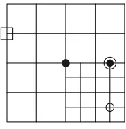
Fig. 1. Different type of grid nodes
In the case of a uniformly refined mesh all nodes are either internal nodes or boundary nodes. In the case of a non-uniformly refined mesh the nodes that lie at the interface of two levels of refinement are termed as either interface nodes or hanging nodes. Interface nodes are nodes which also exist on the next coarser grid and hanging nodes are nodes which only exist on the finer grid. This distinction is important for the understanding of the algorithms that follow.
3.1 Spatial discretization
For all of the computational results presented in this paper second order finite difference schemes have been used. Compact schemes are used for the phase equation in order to reduce the mesh anisotropy influence [19,20]. The mesh data is stored in a quadtree data structure, as in [13,11]. Additional to the information stored in the node list and the element tree, see [13], we also hold for each node a link to their neighbour nodes in order to facilitate the efficient application of different, and especially higher-order, finite difference stencils. Important for the stability of the numerical method is the fact that the interface is always in the refined region. To ensure this, adaptive refinement is used based upon the elementwise gradient criterion
E =Chlvl(|∇φ|+EC|∇U|) (6)
wherehlvl is the element size on the actual refinement level and C, as well as
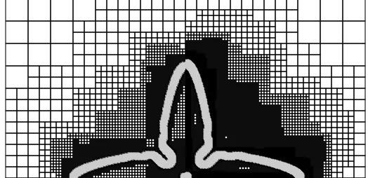
[image:7.612.244.335.19.112.2]Fig. 2. Adaptive meshes after t=2000 for C = 1/2 and left Ec = 0.25 and right
Ec = 1.00, the finest mesh is shaded grey
3.2 Time discretisation
A widely used choice, see [3,8] for example, for temporal discretisation of phase-field models such as (1) and (2) are explicit methods such as the forward Euler scheme. If we rewrite the equations (1) and (2) in operator form
∂φ
∂t =Fφ(t, φ, U),
∂U
∂t =FU(t, U, φ, ∂φ
∂t), (7)
where Fφ and FU are nonlinear differential operators, then the explicit Euler method has the following form
φk+1−φk= ∆tFφ(tk, φk, Uk), (8)
Uk+1−Uk= ∆tFU(tk, Uk, φk,
∂φ
∂t) (9)
for k∈[0, T].
The implementation of the explicit Euler method based upon uniform grids is very straightforward, but for adaptively refined meshes their exist a number of possibilities.
Algorithm 1Explicit Euler method for adaptively refined meshes
1.Go to the finest uniform refined level 2.Solve (8)-(9) for all internal nodes
3.Set up the values on the internal interface nodes of the next finer level by interpolating the values from the coraser mesh
mesh size (h) explicit Euler method
0.781 0.079-0.080
0.391 0.019-0.020
0.195 0.004-0.005
Tab. 1. Maximum stable time step size when using the explicit Euler method on different grid levels
Algorithm 1 shows the implementation used in this work for locally refined spatial meshes. The key point in any such algorithm is the handling of the internal interfaces. The internal interfaces are treated as a Dirichlet boundary for the finer level, with these values obtained by interpolating from the coarser level.
The finer level solution is then obtained only at the internal points. Simple injection is used for the interpolation of the values at the interface nodes from the coarser level, however cubic interpolation is used to obtain Dirichlet values at the hanging nodes. This higher order interpolation is especially needed for the concentration field which is not linear in the internal interface regions. An interesting observation is that to obtain a given accuracy more refinement is needed for the explicit method than for the implicit method, even when higher order interpolation is used at the hanging nodes. The reason is that in the non-linear multigrid solver, which is described later in section 3.4, the hanging nodes are updated at each cycle and the convergence is therefore guaranteed at these nodes.
As already mentioned, the explicit methods suffer from the following time step restriction
∆t≤δh2 (10)
for some constant δ, where ∆t is the time step and h is the minimum ele-ment size. This condition is necessary in order to ensure the stability of the discretisation scheme, and for some non-linear systems the constant δ can be very small, thus leading to excessively small time steps. That is, the time steps are so small that the temporal error is substantially less than the spatial truncation errors.
as used for the majority of calculations in this paper.
In order to overcome this restriction the use of implicit time integration meth-ods is proposed in this paper. These methmeth-ods may be designed to be uncon-ditionally stable, which means that the time step size does not depend on the space step size in order to ensure stability. Our interest is in finding an optimal scheme for which it is possible to set ∆t =δh. The second order Backward Dif-ference Formula (BDF2), combined with the described spatial discretization, would lead to a second order time and space method and so fulfil the desired criterion. This is not true for second order explicit time integration methods, such as Runge-Kutta or the trapezoidal or midpoint rules, see [17], because the stability of these methods are also only preserved by the condition (10). Other classes of implicit higher order time methods can be found for example in [17] or [26].
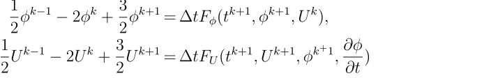
The BDF2 method is an implicit linear 2-step method which takes the follow-ing form when solvfollow-ing (7):
1 2φ
k−1
−2φk+3 2φ
k+1= ∆tF
φ(tk+1, φk+1, Uk), (11) 1
2U k−1
−2Uk+ 3 2U
k+1= ∆tF
U(tk+1, Uk+1, φk
+1
,∂φ
∂t) (12)
[image:10.612.116.463.291.347.2]for k > 1. The first order implicit Euler method is typically used for the first time step (k = 1). It can be shown that the BDF2 method is A stable, see [17], and is therefore widely used for stiff systems of differential equations, for example to simulate chemical reactions or biological phenomena. The advan-tage over one-step second order methods, such as the Crank Nicolson scheme is that only one non-linear solve is required at each time step. The small price that has to be paid for this computational efficiency is that the solutions from the previous two time steps must be saved.
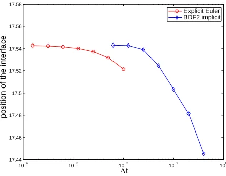
Figure 3 shows a convergence study of the tip position at a fixed time,t= 10.0, for the explicit Euler method and the implicit BDF2 method for decreasing constant time step sizes. The computations are done on uniformly refined grids of dimension [−100,100]2, with an element size ofh= 0.39 and the initial seed
radius is chosen as R0 = 44d0 ≈12.1865. Due to the stability restriction, the
Euler method and can provide comparable accuracy with much larger ∆t.
10−4 10−3 10−2 10−1 100 17.44
17.46 17.48 17.5 17.52 17.54 17.56 17.58
∆ t
position of the interface
[image:11.612.172.395.54.228.2]Explicit Euler BDF2 implicit
Fig. 3. Convergence study of the position of the interface for different time
discreti-sation methods on uniform grids of element size h= 0.39 and at time t= 10.0.
In addition to Figure 3, Table 2 shows the time steps for which the position of the interface has the same accuracy for the explicit and the BDF2 methods. As one can see, the BDF2 method allows ∆t to be up to 80 times larger, for the same accuracy, than the explicit method for this example.
Explicit method BDF2 implicit method
∆t position of the interface ∆t position of the interface
0.01 17.521443 0.05 17.524558
0.00125 17.540187 0.025 17.539207
0.00015625 17.542688 0.0125 17.542740
Tab. 2. Comparison of the time step sizes for which the interface positions are the
same for both methods on a uniform spatial grid with an element size of h = 0.39
and at a final timet= 10.0
3.3 Variable step size control
used in this paper is based upon the following rule: if the estimated local tem-poral error Dk ≤T ol the time step is accepted and the next time step size is increased, whereas ifDk > T ol the step is rejected and retaken with a smaller time step. Let
r= T ol Dk
!1/(p+1)
, (13)
where p is the order of the time discretisation scheme (p = 2 for the BDF2 method and, in the first time stepp= 1 for the implicit Euler method). Then the new time step size ∆tnew is given by
∆tnew = min(rmax,max(rmin, ϑr))∆told, (14)
where the minimal and the maximal time step size growth factor arermin and
rmax respectively, and ϑ is a safety factor, see [17]. In all computations used in this paper the variables are set to rmin = 0.5, rmax= 2.0 and ϑ= 0.8.
The local error estimate is obtained by comparing the solution of the BDF2 method and the solution obtained by using a first order method. (In the first time step the local error is estimated by comparing the solution φ1
im using the implicit Euler method with the solution of the explicit Euler method φ1
ex = φ0 + ∆t0Fφ(φ0, U0): the local error estimator is given then as D0 =
1
2||φ1im−φ1ex)||∞ .) In this work the implicit Euler method is used for the first order scheme, as derived in [17], leading to the following estimate
Dk=
r 1 +r||φ
k+1
−(1 +r)φk+rφk−1
||∞, (15)
where r is the steps size ratio ∆tk/∆tk−1. Tests show that for the equations (1)-(2) it is sufficient to base the time step control only on the phase variable due to the fact that the two equations are of the same type. This is different to most thermal models for the simulation of pure material solidification, see [18], where the temperature equation and the phase equation are of a differ-ent type, with differdiffer-ent requiremdiffer-ents on the time step size. To overcome this difficulty the authors in [11] use a second order time discretisation scheme for the temperature equation and a first order scheme for the phase equation.
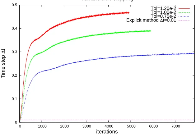
0 0.1 0.2 0.3 0.4 0.5
0 1000 2000 3000 4000 5000 6000 7000
Time step
∆
t
iterations Variable time stepping
[image:13.612.128.443.33.252.2]Tol=1.20e-2 Tol=1.00e-2 Tol=0.75e-2 Explicit method ∆t=0.01
Fig. 4. The evolution of the time step size fort= 0. . .2000, and a minimal element
size ofh= 0.39, for different tolerances and in comparison to the constant step size
∆t= 0.01 for the explicit method
step size of the BDF2 method with T ol= 1.2e−2 the step size of the explicit Euler method is, forh= 0.39, 45 times smaller.
3.4 Non-linear multigrid solver
When using implicit time discretisation methods it is necessary to solve a system of non-linear algebraic equations at each time step. multigrid methods are among the fastest available solvers for large sparse systems of linear or non-linear algebraic equations and are based upon two principles; the coarse grid principle and the smoothing principle, see for example [21–23]. For the coarse grid correction one has to define grid transfer operators to transfer the solution and the residual from the fine to the coarse grid, and the solution from the coarse to the fine grid. In the examples given here bilinear interpolation is used for the coarse to fine grid transfers and injection is used for the fine to coarse grid transfers. For the smoothing principle a basic iteration method for smoothing the error is used. One of the simplest possibilities is a pointwise non-linear weighted Jacobi smoother, which is used here for the Phase equation:
φkij+1,n+1 =φkij+1,n−ω (F⋆
φ(φ k+1,n
ij , Uijk)−(φkj +14φ
k−1 )) ∂
∂φijF
⋆ φ(φ
k+1,n ij , Uijk)
where
Fφ⋆(φk+1, Uk) = −∆t 2 Fφ(t
k+1, φk+1, Uk) +3 4φ
k+1, (17)
which follows from equation (11). The advantage of using a Jacobi smoother is thatψin (1) has to be calculated only once per iteration. For the concentration equation a pointwise non-linear weighted Gauss-Seidel smoother is used:
Uijk+1,n+1=Uijk+1,n+1−ωF
⋆ U(U
k+1,n+1
ij , φkij+1, ∂φk+1
ij
∂t )−(U k j +14U
k−1 )
∂ ∂UijF
⋆ U(U
k+1,n+1
ij , φkij+1, ∂φk+1
ij
∂t )
, (18)
where
FU⋆(Uk+1, φk+1,∂φ
k+1
∂t ) =− ∆t
2 FU(t
k+1, Uk+1, φk+1,∂φk+1
∂t ) + 3 4U
k+1.(19)
For both smoothers the derivatives of the discretisation operators with re-spect to the system variable at each point is needed. In order to simplify these derivatives, central difference schemes are used to approximate the first and second derivatives in both directions, so that the derivative is zero, e.g.
∂ ∂φij h∂φ ∂x i ij
= 0 with h∂φ∂xi i,j =
1
2h(φi+1,j−φi−1,j). The derivative of the right-hand side of (17) with respect to φij is therefore given as
∂F⋆ φ(φ, U)
∂φij ≈
−∆t 2A2(ψ
ij)
(
A(ψij)2
∂ ∂φij
∇2
hφij
+ 1−3φ2
ij−
2λ(θf ix+Mc∞Uij) (−φij + 2φ3ij)+
A′2
(ψij) +A(ψij)A ′′
(ψij)
1
|∇hφij|2
(
φ2x∂φyy ∂φij
+φ2y∂φxx ∂φij −
2φxφy
∂φxy
∂φij
))
+ 3 4
where∇2h is the discrete Laplace operator, in this case the second order com-pact nine point stencil, see for example [27]. The same procedure applied to the right hand-side of (19) gives
∂F⋆ U(φ, U)
∂Uij ≈
−∆t 1 +k−(1−k)φij
(
D 1−φij 2
∂ ∂Uij
∇2hUij
!!
+
1
2√2 (1−k) ∂ ∂x
∂φ ∂t
φx
|∇hφij|
! + ∂ ∂y ∂φ ∂t φy
|∇hφij|
!!!
1
2(1−k) ∂φ
∂t
)
+3 4
where, for example φx, is the notation for the first derivative ∂φ∂xij.
On the basis of the described smoothers and transfer operators a multigrid solver for adaptive refined meshes has been developed based upon the Full Approximation Scheme (FAS) for resolving the non-linearity, see [24], and the adaptive multigrid approach of [21]. Another multigrid methods for local re-fined meshes is the Fast Adaptive Composite Grid method which is described in [23,25]. Note that although the smoothers (16) and (18) have been writ-ten separately, the nonlinear system that is solved is a single system for all unknowns φk+1
ij and Uijk+1. The number of pre- and post-smooths applied is typically two, however other alternatives are presented in Table 5. Note that the multigrid convergence rate depends on a number of factors, including: the transfer operators; the smoother; the number of post and pre smooths; and also on the iteration form. Table 3 shows convergence rates for different iter-ation forms and different pre and post smoothing steps at a fixed time and a constant time step size of ∆t = 0.05 on uniform grids with size h = 0.78. The notation V(2,1), for example, represents a V-cycle with 1 post and 2 pre smoothing steps. The convergence rate is calculated by iterating until a resid-ual of less than 1e−10 is reached and then the proportion of the residual ofφ at the penultimate and last steps is calculated, measured in the Infinity-norm. The number of iterations needed to reach a residual of less than 1e−10 is equal to the number of cycles in the Table. As one can see the V-cycle form with 2 post and 2 pre smoothing steps performed best in terms of convergence rate, number of cycles and execution time.
iteration form convergence rate no. of cycles time (sec)
V(1,1) 0.008789 5 2.3915
V(2,1) 0,000872 4 2.4667
V(2,2) 0.000098 3 2.3021
W(1,1) 0.008788 5 3.3234
W(2,2) 0.000097 3 3.1040
Tab. 3. Statistic of the convergence rate, number of cycles and the execution time for different types of iteration form
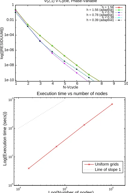
the convergence rate even for this highly non-linear problem.
An implication of this is that the execution time versus the number of nodes should scale linearly, and this optimal behaviour is indeed observed in Figure 5b.
1e-10 1e-08 1e-06 1e-04 0.01 1
1 2 3 4 5 6 7 8 9 10
log(||RESIDUUM||)
N-Vcycle V(2,1) V-Cycle, Phase-Variable
h = 1.56 h = 1.56 (adaptive) h = 0.78 h = 0.78 (adaptive) h = 0.39 h = 0.39 (adaptive)
104 105 106
100 101 102 103
Log(Number of nodes)
Log(Execution time (secs))
Execution time vs number of nodes
Uniform grids Line of slope 1
Fig. 5. a)Residual of the phase variable at a fixed time for different mesh levels as well as uniformly and nonuniformly refined meshes; b)shows the execution time for various system sizes
4 Results
This section presents a selection of typical results for the solution of (1)-(2), concentrating mainly on the comparison between the explicit Euler method and the implicit BDF2 time discretisation method. The following aspects are considered:
1. The influence of the refinement on the accuracy.
2. The influence of the choice of the time step size on the accuracy, and 3. The execution times of both methods.
[image:16.612.182.394.101.420.2]dendritic growth simulation is undertaken with the model parameters given in section 2. The only free parameter to choose is the coupling parameterλ, which depends on the choice of the diffusivity coefficient D, see (3). This parameter is set to D = 2 in these simulations, whereby it follows that λ = 3.1913 and the capillarity length d0 = 0.27696. The rectangular computational domain
Q is chosen as Q= [−400,400]2 with Dirichlet boundary conditions. On the
boundaries φis set to be −1 and the concentration fieldU is considered to be zero. The phase field is initialised as φ =−tanh(β(x2 +y2−R2
0)), where R0
is the radius of the initial seed andβ a constant to control the steepness, and the concentration U is initialised to zero in the whole domain.
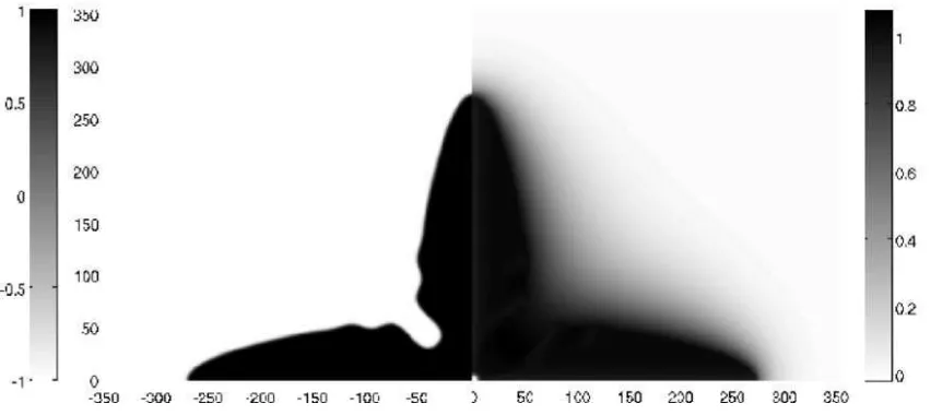
[image:17.612.92.518.339.529.2]A typical simulation result for a four-fold symmetric alloy dendrite growing in an undercooled melt is shown in Figure 6. The contour plots show, on the left-hand side, the phase variable and, on the right-left-hand side, the concentration field at t = 1800. At this time the tip velocity has reached a steady state. In those regions where the phase variable forms a very steep interface the concentration field is more slowly varying and is only very sharp in front of the tip. This illustrates the need for local mesh refinement, see section 3 and Figure 2. The influence that the adaptive refinement has on the simulation results is discussed in the next section.
Fig. 6. The interface shape of an alloy dendrite aftert= 1800; the left and the right
box show the contours of the phase variableφand the contours of the dimensionless
concentration field U, respectively
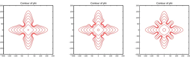
In order to simulate a pure four-fold symmetry the radius of the initial solid seed is taken as R0 = 14d0 in all cases. Figure 7 shows a study of how the
radius of the initial seed influences the shape of the dendrite. If the initial radius is chosen to be larger than R0 = 28d0 then the dendrite no longer
Contour of phi
−200 −150 −100 −50 0 50 100 150 200
−200 −150 −100 −50 0 50 100 150 200
Contour of phi
−200 −150 −100 −50 0 50 100 150 200
−200 −150 −100 −50 0 50 100 150 200
Contour of phi
−200 −150 −100 −50 0 50 100 150 200
[image:18.612.119.498.21.140.2]−200 −150 −100 −50 0 50 100 150 200
Fig. 7. The evolution of the interface for a different radius of the initial solid seed
a) R0 = 14d0 b)R0 = 28d0 and c) R0= 44d0
4.1 Adaptive remeshing
In this section we compare results obtained on uniform meshes and on adap-tively refined meshes and study what influence the adaptive refinement has on different parameters for different discretisation methods. All the results shown next are for meshes with a minimum element size ofh= 0.78. For the explicit Euler method a constant step size of ∆t= 0.05 was chosen, which is slightly less than the maximum stable time step, see Table 1. For the BDF2 method the error tolerance, T ol in (13), was fixed as 1e−2.
The first test was undertaken on a smaller domain Q= [−200,200]2 to show
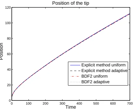
that the adaptive refinement generally does not have an effect on the simula-tion results. To demonstrate the same accuracy for both uniform and adaptive refinement Figure 8 shows the position of the tip along the x-axis as a function of time. Since the computation of the tip velocity and the curvature depends on the position of the tip it is important to demonstrate that the tip position is the same.
0 100 200 300 400 500 600 700 0
20 40 60 80 100 120
Position of the tip
Time
Position
[image:19.612.179.394.24.202.2]Explicit method uniform Explicit method adaptive BDF2 uniform BDF2 adaptive
Fig. 8. Comparison of the tip position computed on uniformly and adaptively refined meshes using the explicit Euler time integration scheme and the BDF2 method
For the rest of this paper only adaptively refined meshes will be consid-ered. This is because it becomes excessively expensive to compute on uniform meshes as h is reduced. For example, with a minimum element size of 0.098, which is comparable to a uniform mesh with 67 million nodes, it is impossible to solve on a single workstation.
As already indicated above, the choice of the adaptive refinement parameters have an influence on the results in both methods. The explicit method is particularly sensitive to the refinement scheme due to the more complicated handling of the internal interface nodes, as discussed in section 3.2. Even if cubic interpolation is used at the internal interfaces more refinement is needed in order to reproduce the same results as with the implicit BDF2 method, where the interface nodes are incorporated very naturally into the multigrid solver, see for example [21]. Table 4 shows a parameter study, and how the parameters influence the position and the velocity of the tip aftert= 1800 on a domain Q= [−400,400]2 with h = 0.78.
method parameters position velocity
explicit Euler C = 1/2, Ec = 1.0 230.92387 0.106260
C = 1.0, Ec = 1.0 235.32227 0.108935
C = 2.0, Ec = 1.0 236.45504 0.109486
implicit BDF2 C = 1/2, Ec = 0.75 234.69686 0.109041
C = 1.0, Ec = 0.75 236.50597 0.109649
Tab. 4. Position of the tip and the tip velocity at t= 1800 for different refinement
T ol position velocity time step
1.20e-2 234.72354 0.109029 ≈0.49
1.00e-2 234.69686 0.109041 ≈0.40
0.75e-2 234.84339 0.109166 ≈0.30
Tab. 5. Position of the tip and the tip velocity at t = 1800 for different error
tolerances in the time step control as well as the time step size
In Table 4 the parameter Ec are held constant and the parameter C, which is global parameter and leads to more refinement on all levels, is varied. Both methods converge to the same position but the explicit method needs more refinement than the BDF2 method. In order to compare the results for both methods the parameter values that are chosen in all later studies are: C = 2.0, Ec = 1.0 for the explicit Euler scheme, C = 1.0, Ec = 0.75 for the BDF2 method.
4.2 Parameter studies
[image:20.612.211.363.571.638.2]Before reaching the final comparison in the next section one further parameter study is undertaken, concerning the time step control and the multigrid solver tolerance for the BDF2 method. The simulation parameters are as stated in the previous section.
Table 5 shows the position of the tip and the tip velocity at t = 1800 for different tolerances T ol in the step size control. When the tolerance is small then the time steps become smaller, see Figure 4. However, as one can see, the difference between results computed with different tolerances are marginal but the difference in the time step sizes are quite significant. For example the change of the tip position between the choiceT ol = 1.2e−2 andT ol= 0.75e−2 is only 0.05% but the final time step size forT ol = 1.2e−2 is 63% larger than the final time step size when using T ol = 0.75e−2. This leads to an huge drop in the number of time steps and so in the overall execution time.
A similar conclusion can be reached by studying the dependence of the multi-grid solver tolerance Stol on the simulation results. Table 6 shows the tip
Stol position velocity
1e-7 234.74028 0.109042
1e-5 234.69686 0.109041
Tab. 6. Position of the tip and the tip velocity for different solver tolerances after
position and the tip velocity for two different solver tolerances, all other pa-rameters held to be the same. As one can see the solver tolerance does not influence the results significantly, there is only a 0.018% difference in the position of the tip between both. Consequently, for subsequent calculations Stol= 1e−5 chosen since the number of multigrid iterations, which depends on the chosen solver tolerance, does have a significantly impact on the total execution time.
After studying the different parameters which could have an effect on the simulation results we come now to a final comparison of the explicit and the implicit methods.
4.3 Comparison of the explicit Euler method and the implicit BDF2 method
A graphical comparison of a selection of results on adaptively refined meshes are shown in Figure 9. The top left figure shows the position of the tip of a dendrite growing along the x-axis versus time. The top right figure is the tip
0 200 400 600 800 1000 1200 1400 1600 1800
0 50 100 150 200 250 Time
Position of the tip
Tip position
Explicit method BDF2 method
0 200 400 600 800 1000 1200 1400 1600 1800
0 0.2 0.4 0.6 0.8 1 1.2 1.4 Time
Velocity of the tip
Tip velocity
Explicit method BDF2 method
0 200 400 600 800 1000 1200 1400 1600 1800
1 2 3 4 5 6 7 Time
Curvature of the tip
Radius of Curvature
Explicit method BDF2 method
0 200 400 600 800 1000 1200 1400 1600 1800
0 0.05 0.1 0.15 0.2 0.25 0.3 0.35 0.4 0.45 Time ∆ t Time steps
[image:21.612.106.494.314.616.2]position velocity curvature total time (hours)
explicit Euler 236.45504 0.109486 6.034250 11.8
implicit BDF2 236.50597 0.109649 6.004577 11.5
Tab. 7. Comparison of the position, velocity and radius of the tip on the x-axis after
t= 1800 and the total execution time
velocity versus time and the bottom left graph shows the tip radius versus time. Finally the bottom right figure shows the evolution of the time step size for the BDF2 method. All simulations are evaluated until t = 1800 where a steady state tip velocity is reached, which is equivalent to a dimensionless time of tD/d2
0 ≈ 47000. As one can see both methods produce the same
results, with the respective curves lying on top of each other. This correlation is strengthened by a direct comparison of the steady state results in Table 7. The total execution time is additionally shown in this table. From Table 5 it is known that the time step at the end of the simulation is ∆t ≈ 0.4 for the BDF2 scheme in comparison to the constant time step of ∆t = 0.05 necessary for stability of the explicit Euler method. In order to make the time comparison as fair as possible therefore mesh refinement is only undertaken every 10 time steps with the explicit method, compared to each time step in the BDF2 method.
The results clearly demonstrate that both methods produce the same simula-tion results. Furthermore, the spatial mesh level with a minimum element size ofh= 0.78 is the first level for which the implicit BDF2 method is faster than the explicit Euler method on adaptively refined meshes. However, the conver-gence study of the steady-state tip velocity in the next section demonstrates that a spatial step size of at least h= 0.39 is needed to approximate the test problem considered here with sufficient accuracy. Such a decrease of the step size has a significant impact on the total execution time for both methods but the time increase for the explicit method is much greater than for the implicit method. This is because the stability restriction for the explicit method means that one has to quarter the time step whenever the minimum element size is halved. Based on the fact that, in the adaptive meshing, the number of nodes only doubles or triples every time the minimum element size is halved, the total execution time for the explicit Euler method should go up by a factor of 8 to 12. However, for the BDF2 method the execution time only increases by factor of at most 4 to 6 because of the variable step size control.
of 10, although the execution time increases from h = 078 to h = 0.78 by a factor of 11.9. To complete an explicit simulation on meshes with a step size of h = 0.097 would require an execution time of more than 12000 hours. For the same system size the BDF2 method needs a little more than 400 hours, which is about 30 times less.
10−1 100
100 101 102 103 104
Execution time
log(h)
log(Execution Time (hours))
Explicit Euler method (data) Explicit Euler method (extrapolation) BDF2 method (data)
[image:23.612.167.399.126.323.2]Line of slope −1
Fig. 10. The execution time for both methods and various system sizes
4.4 Convergence behaviour
To complete this presentation of results, this section examines the convergence behaviour of the simulations. All subsequent simulations are performed with the BDF2 method on meshes with a minimum element size of less than or equal to h = 0.78. Figure 11 shows the progression of the tip position and the tip velocity over time for different maximum refinement levels. Both pa-rameters converge as the meshes become finer. Only the results computed on meshes with a step size of h = 0.78 stand out at this graph resolution, thus demonstrating that a finer grid spacing is essential for accurate predictions.
0 200 400 600 800 1000 1200 1400 1600 1800 0
50 100 150 200 250 300
Time
Position
Tip position
BDF2 (h=0.78) BDF2 (h=0.39) BDF2 (h=0.19) BDF2 (h=0.097)
0 200 400 600 800 1000 1200 1400 1600 1800
0 0.2 0.4 0.6 0.8 1 1.2 1.4
Time
Velocity
Tip velocity
[image:24.612.101.479.26.168.2]BDF2 (h=0.78) BDF2 (h=0.39) BDF2 (h=0.19) BDF2 (h=0.097)
Fig. 11. Convergence study of the dimensionless tip position and tip velocity up to
t= 1800 for decreasing element sizes
0 0.1 0.2 0.3 0.4 0.5 0.6 0.7 0.8 0.9 0.01
0.011 0.012 0.013 0.014 0.015 0.016 0.017 0.018 0.019 0.02
Tip velocity
h
Vtip d0
/D
Fig. 12. Convergence study of the dimensionless tip velocity att= 1800 for
decreas-ing element sizes
5 Conclusions
This paper presents an efficient fully adaptive numerical scheme for the simu-lation of dendritic alloy growth in a undercooled melt in two dimensions. The phase-field model used to demonstrate the method is a variation of the coupled thermal-solute model, published in [3], for the simulation of isothermal growth. In order to solve efficiently on meshes with a very fine spatial resolution adap-tive meshing and a second-order implicit time discretisation scheme are used and coupled with variable time step size control. This combination reduces the execution time drastically compared to explicit time integration methods since their is no artificial stability restriction imposed on the time step size, see Figure 10. To solve the intermediate approximations in the implicit BDF2 method a robust multigrid solver is essential, the FAS scheme applied on the adaptive grids in this work shows excellent h-independent convergence rates.
[image:24.612.180.383.222.380.2]good agreement with results published in [3] and [8]. By using the fully implicit approach it has been possible to compute efficiently using minimum element sizes of less than 0.1. In order to achieve this accuracy on uniform meshes one would need lattice with 213×213 nodes, and the use of explicit time stepping
would not be practical.
This is the first paper to couple the use of adaptivity in space and time with implicit methods and the use of multigrid solvers for the simulation of solidifi-cation using Phase-field models. Numerous other phase-field models exist and further studies may be undertaken, including the application of this numeri-cal method to the fully-coupled thermal-solute model, which exhibits diffusion effects on different time scales, thus making the potential advantages of the proposed approach even greater.
6 Acknowledgements
This work was supported by EPSRC Grant No. GR/T10374/01. We thank Dr. Alison Jones for providing the initial version of our mesh adaptivity routines [13].
References
[1] R. Kobayashi, Modeling and numerical simulations of dendritic crystal growth, Physica D 63 (1993) 410-423
[2] W.J. Boettinger, J.A. Warren, C. Beckermann, and A. Karma, Phase-Field Simulation of Solidification, Annu. Rev. Mater. Res 32 (2002) 163-194, doi: 10.1146/annurev.matsci.32.101901.155803.
[3] J.C. Ramirez, C. Beckermann, A. Karma, and H.-J. Diepers, Phase-field modeling of binary alloy solidification with coupled thermal heat and solute diffusion, Physical Review E 69 (2004), doi: 10.1103/PhysRevE.69.051607.
[4] A.M. Mullis, An extension to the Wheeler phase-field model to allow decoupling of the capillary and kinetic anisotropies, Eur. Phys. Journal B 41 (2004) 377-382, doi: 10.1140/epjb/e2004-00330-7.
[5] A.M. Mullis, Quantification of mesh induced anisotropy effects in the phase-field method, Computational Materials Science 36 (2006) 345-353, doi:10.1016/j.commatsci.2005.02.017
[7] S.G. Kim, W.T. Kim, and T. Suzuki, Phase-field model for binary alloys, Physical Review E 60 (1999) 7186-7197
[8] A. Karma,
Phase-Field Formulation for Quantitative Modeling of Alloy Solidification, Physical Review Letters 87 (2001), doi: 10.1103/PhysRevLett.87.115701.
[9] A. Schmidt, Computation of Three Dimensional Dendrites with Finite Elements, Journal of Computational Physics 125 (1996)
[10] R.J. Braun, and B.T. Murray, Adaptive phase-field computations of dendritic crystal growth, Journal of Crystal Growth 174 (1997) 41-53
[11] N. Provatas, N. Goldenfeld, J. Dantzig, Adaptive Mesh Refinement Computation of Solidification Microstructures Using Dynamic Data Structures, Journal of Computational Physics 148 (1999) 265-290
[12] B. Nestler, D. Danilov, and P. Galenko, Crystal growth of pure substances: Phase-field simulations in comparison with analytical and experimental
results, Journal of Computational Physics 207 (2005) 221-239, doi:
10.1016/j.jcp.2005.01.018.
[13] A.C. Jones, A Projected Multigrid Method for the Solution of Nonlinear Finite Element Problems on Adaptively Refined Grids, Ph.D. thesis, School of Computing, University of Leeds, 2005
[14] W.L. George, and J.A. Warren, A Parallel 3D Dendritic Growth Simulator Using the Phase-Field Method, Journal of Computational Physics 177 (2002) 264-283, doi: 10.1006/jcph.2002.7005.
[15] C.W. Lan, Y.C. Chang, and C.J. Shih, Adaptive phase field simulation of non-isothermal free dendritic growth of a binary alloy, Acta Materialia 51 (2003) 1857-1869, doi: 10.1016/S1359-6454(02)00582-7
[16] P. Zhao, M. V´enere, J.C. Heinrich, and D.R. Poirier, Modeling dendritic growth of a binary alloy, Journal of Computational Physics 188 (2003) 434-461, doi: 10.1016/S0021-9991(03)00185-2.
[17] W. Hundsdorfer, J.G. Verwer, Numerical Solution of Time-Dependent
Advection-Diffusion-Reaction Equations, Springer Verlag, 2003
[18] A. Karma, W.J. Rappel, Phase-field method for computationally efficient modeling of solidification with arbitrary interface kinetics, Physical Review E 53 (1996)
[19] A. Karma, W.J. Rappel ,Quantitative phase-field modelling of dendritic growth in two and three dimensions, Physical Review E 57 (4) (1998)
[20] B. Echebarria, R. Folch, A. Karma, M. Plapp, Quantitative phase-field model of alloy solidification, Physical Review E 70 (2004)
[22] W. Hackbusch, Multi-Grid Methods and Applications, Springer Series in Computational Mathematics (Springer-Verlag, Berlin/Heidelberg, 1985)
[23] W.L. Briggs, V.E. Henson, and S.F. McCormick, A Multigrid Tutorial, SIAM, Philadelphia, 2nd edition, 2000
[24] A. Brandt, Multi-Level Adaptive Solutions to Boundary-Value Problems, Mathematics of Computation 31 (1977) 333-390
[25] S.McCormick, and J. Thomas, The Fast Adaptive Composite Grid (FAC) Method for Elliptic Equations, Mathematics of Computation 46 (1986) 439-456
[26] J. Lang, Adaptive Mulitlevel Solution of Nonlinear Parabolic PDE systems:
Theory, Algorithm and Application, Springer, 2001
[27] W. Hackbusch, Theorie und Numerik elliptischer Differentialgleichungen,