Unfolding Kernel Embeddings of Graphs : Enhancing Class Separation through Manifold Learning

(1)

This is a repository copy of Unfolding Kernel Embeddings of Graphs : Enhancing Class Separation through Manifold Learning.

White Rose Research Online URL for this paper: http://eprints.whiterose.ac.uk/84841/

Version: Accepted Version

Article:

Rossi, Luca, Torsello, Andrea and Hancock, Edwin R orcid.org/0000-0003-4496-2028 (2015) Unfolding Kernel Embeddings of Graphs : Enhancing Class Separation through Manifold Learning. Pattern Recognition. pp. 3357-3370. ISSN 0031-3203

https://doi.org/10.1016/j.patcog.2015.03.018

[email protected] Reuse

Items deposited in White Rose Research Online are protected by copyright, with all rights reserved unless indicated otherwise. They may be downloaded and/or printed for private study, or other acts as permitted by national copyright laws. The publisher or other rights holders may allow further reproduction and re-use of the full text version. This is indicated by the licence information on the White Rose Research Online record for the item.

Takedown

If you consider content in White Rose Research Online to be in breach of UK law, please notify us by

(2)

Unfolding Kernel Embeddings of Graphs:

Enhancing Class Separation through Manifold Learning

Luca Rossi 1∗_{, Andrea Torsello}2_{, Edwin R. Hancock}3 1

School of Computer Science, University of Birmingham, UK 2

Department of Environmental Science, Informatics, and Statistics, Ca’ Foscari University of Venice, Italy

3

Department of Computer Science, The University of York, York YO10 5DD, UK

Abstract

In this paper, we investigate the use of manifold learning techniques to enhance the

separa-tion properties of standard graph kernels. The idea stems from the observasepara-tion that when

we perform multidimensional scaling on the distance matrices extracted from the kernels,

the resulting data tends to be clustered along a curve that wraps around the embedding

space, a behaviour that suggests that long range distances are not estimated accurately,

resulting in an increased curvature of the embedding space. Hence, we propose to use a

number of manifold learning techniques to compute a low-dimensional embedding of the

graphs in an attempt to unfold the embedding manifold, and increase the class separation.

We perform an extensive experimental evaluation on a number of standard graph datasets

using the shortest-path [1], graphlet [2], random walk [3] and Weisfeiler-Lehman [4] kernels.

We observe the most significant improvement in the case of the graphlet kernel, which fits

with the observation that neglecting the locational information of the substructures leads to

a stronger curvature of the embedding manifold. On the other hand, the Weisfeiler-Lehman

kernel partially mitigates the locality problem by using the node labels information, and

thus does not clearly benefit from the manifold learning. Interestingly, our experiments also

show that the unfolding of the space seems to reduce the performance gap between the

examined kernels.

Keywords: Kernel Learning, Kernel Unfolding, Graph Kernels, Manifold Learning

(3)

1. Introduction

Graph-based representations have become increasingly popular due to their ability to

characterize in a natural way a large number of systems which are best described in terms

parts and binary relations. Concrete examples include the use of graphs to represent

shapes [5], metabolic networks [6], protein structure [7], and road maps [8]. However, the

rich expressiveness and versatility of graphs comes at the cost of added complexity and

a reduced toolset of available pattern analysis algorithms. In fact, our ability to analyse

data abstracted in terms of graphs is severely limited by the restrictions posed by standard

pattern recognition techniques, which require data to be representable in a vectorial form.

There are two reasons why graphs are not easily reduced to a vectorial form: First, there is

no canonical ordering for the nodes in a graph, unlike the components of a vector. Hence,

correspondences to a reference structure must be established as a prerequisite. Second, the

variation in the graphs of a particular class may manifest itself as subtle changes in structure.

Hence, even if the nodes or the edges of a graph could be encoded in a vectorial manner,

the vectors would be of variable length, thus residing in different spaces.

The first 30 years of research in structural pattern recognition have been mostly

con-cerned with the solution of the correspondence problem as the fundamental means of

assess-ing structural similarity [9]. With the similarity at hand, similarity-based pattern recognition

techniques such as the nearest neighbour rule can be used to perform recognition and

classi-fication tasks, or graphs may be embedded in a low-dimensional pattern space using either

multidimensional scaling or alternative non-linear manifold leaning techniques.

Another alternative is to extract feature vectors from the graphs providing a

pattern-space representation. There are a number of ways in which this can be done: One approach

is to extract structural or topological features from the graphs under study. Graph

spec-tral features extracted from the eigenvalues and eigenvectors of the adjacency or Laplacian

matrices have been shown to be effective here [10, 11]. Again, manifold learning techniques

have been used in the literature to provide a way to unfold the pattern space and map the

(4)

data onto low-dimensional spaces where the structural classes are well separated.

The famous kernel trick [12] has shifted the problem from the vectorial representation of

data, which now becomes implicit, to a similarity representation. This has allowed standard

learning techniques to be applied to data for which no easy vectorial representation exists.

More formally, once we define a positive semi-definite kernel k : X×X → R on a set X,

there exists a mapφ:X → H into a Hilbert space H, such that k(x, y) =φ(x)⊤φ(y) for all x, y ∈ X. Also, given the kernel value between φ(x) and φ(y) one can easily compute the

distance between them by noting that||φ(x), φ(y)||2 ₌_φ(x)⊤_φ(x)+_φ(y)⊤_φ(y)₋_2φ(x)⊤_φ(y). Thus, any algorithm that can be formulated in terms of dot products between the input

vectors can be applied to the implicitly mapped data points through the direct substitution

of the kernel for the dot product. For this reason, in recent years pattern recognition has

witnessed an increasing interest in structural learning using graph kernels. However, due to

the rich expressiveness of graphs, this task has also proven to be difficult, with the problem

of definingcompletekernels, i.e., ones where the implicit mapφ is injective, sharing the same

computational complexity of the graph isomorphism problem [13].

While the graph kernels proposed in the literature provide effective ways to generate

implicit embeddings, there is no guarantee that the data in the Hilbert space will exhibit

better class separation. This is of course a consequence of the complexity of the structural

embedding problem and the limits for efficient kernel computations already analysed by

G¨artner et al. [13]. One evidence of this is the fact that the multidimensional scaling

embeddings of several graph kernels show the so-called horseshoe effect [14] (see Figure 1),

i.e., the data tends to cluster tightly along a curve that wraps around the embedding space.

This particular behaviour is typically produced by a consistent underestimation of the real

distances of the problem, i.e., the geodesic distances on the manifold, and it implies that

the data gets placed onto a highly non-linear manifold embedded in the Hilbert space. The

horseshoe is in fact the locus of intersection between the manifold and the plane used to

visualise the data, and the high curvature is a result of the dimensionality compression on

the data, which reduces the degrees of freedom of the points and forces them to cluster

(5)

−100 0 100 200 300 −20

−10 0 10 20 30

1st Leading Dimension

2nd Leading Dimension

(a) Shortest-path

−0.5 0 0.5 1

−0.4 −0.2 0 0.2 0.4 0.6

(b) Graphlet

−20 −10 0 10 20 30

−1 −0.5 0 0.5 1 1.5

(c) Random walk

−5 0 5 10 15

−4 −2 0 2 4 6

(d) W L1

−5 0 5 10 15

−4 −2 0 2 4 6 8

(e) W L2

−5 0 5 10 15

−4 −2 0 2 4 6 8

[image:5.595.71.526.107.397.2]

(f) W L3

Figure 1: The MDS embeddings of the shortest-path [1], graphlet [2], random walk [3] and

Weisfeiler-Lehman [4] kernels (withh= 1,2,3) on the COIL dataset.

of kernel normalization, a common procedure through which the data points are projected

from the Hilbert space onto the unit sphere. This in turn creates an artificial curvature of

the space that can create or exacerbate the observed horseshoe effect. Note, however, that

while in general the non-linearity of the mapping is used to improve local class separability,

a large global curvature can result in a folding of the manifold that can reduce long range

separability.

For this reason, it is natural to investigate the impact of the locality of distance

infor-mation on the performance of these kinds of kernels. To this end, given a set of graphs, we

investigate the use of several manifold learning techniques to embed the graphs onto a

low-dimensional vectorial space, in an attempt to unfold the embedding manifold, and increase

class separation. More specifically, we investigate the use of four popular non-linear

mani-fold learning techniques, namely Isomap [15], Laplacian Eigenmaps [16], Diffusion Maps [17]

(6)

[image:6.595.86.516.123.299.2]

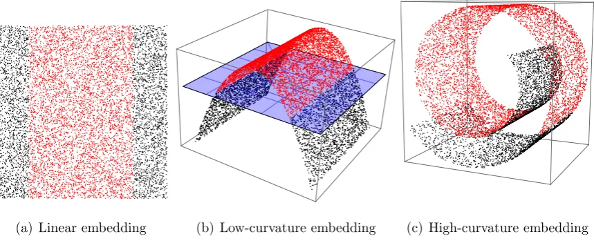
learn-(a) Linear embedding (b) Low-curvature embedding (c) High-curvature embedding

Figure 2: Example of reduced linear separability due to high curvature of the embedding. In the linear

embedding case the data is not separable, introducing a non-linear mapping to a low-curvature manifold

renders the data linearly separable. However, mapping to a high global curvature manifold (e.g. the famous

swissroll manifold) results in a reduced linear separability of the data. Furthermore, the higher the curvature

the less separable the data is.

ing problem from radically different angles, with Isomap attempting to preserve the global

distances and LLE trying to maintain the local neighbourhood geometry.

Experiments on several standard datasets demonstrate that, as expected, the

improve-ment is kernel and dataset dependent, with some kernels and datasets generally gaining very

significant improvements in performance, while other not exhibiting significant variation or

even modest reduction. Most importantly, the unfolding of the manifold invariably reduces

the performance gap between the kernels examined. This suggests that the instances of

ker-nels in the literature do not differ by any intrinsic difference in descriptive power, but in the

level of warping of the embedding space. See Figure 2 for an example where the non-linear

mapping to a high-curvature manifold reduces the linear separability of data.

The remainder of this paper is organized as follows: Section 2 introduces some related

work in graph kernels and manifold learning, while Section 3 illustrates the unwrapping idea

and provide a more in-depth description of the kernels and manifold learning techniques

used in this study. Section 4 illustrates the experimental results, while Section 5 discusses

(7)

2. Related Works

Many different graph kernels have been proposed in the literature, and they are generally

instances of the family of R-convolution kernels first introduced by Haussler [22]. The

fundamental idea is that of decomposing two discrete objects and comparing some simpler

substructures. Generally speaking, most R-convolution kernels simply count the number of

isomorphic substructures in the two graphs being compared, and differ mainly by the type

of substructures used in the deconvolution and the algorithms used to count them efficiently.

For example, Kashima et al. [3] propose to count the number of common random walks

between two graphs. This kernel, however, is subject totottering. That is, a walk is allowed

to go back and forth along a single edge multiple times, thus reducing the discriminative

power of the kernel. A solution to this is proposed by Mahe et al. [47], who modify the

standard random walk model by preventing the walk from returning to a vertex that has

just been visited. Borgwardt and Kriegel [1] measure the similarity by counting the numbers

of pairs of shortest paths of the same length in the graphs. Shervashidze et al. [2], on the

other hand, count the number of graphlets, i.e. subgraphs with k ={13,4,5} nodes. More

recently, Shervashidze et al. [4] have developed a subtree kernel on subtrees of limited size.

They compute the number of subtrees shared between two graphs using the

Weisfeiler-Lehman graph invariant. Another kernel based on subtrees enumeration is that of Ga¨uzere

et al.[48]. More specifically, Ga¨uzere et al. define the similarity between two graphs in terms

by decomposing them in bags of treelets, i.e., acyclic and unlabeled trees whose maximal

size is equal to 6. Ralaivola et al. [49], on the other hand, develop a series of kernels by

exploiting specific structural properties of graphs arising in the domain of organic chemistry.

Aziz et al. [23] have defined a backtrackless kernel on cycles of limited length. They compute

the kernel value by counting the numbers of pairs of cycles of the same length in a pair of

graphs. Costa and Grave [24] have defined a so-called neighbourhood subgraph pairwise

distance kernel by counting the number of pairs of isomorphic neighbourhood subgraphs.

Recently, Kriege et al [25] counted the number of isomorphisms between pairs of subgraphs,

(8)

partially labelled graphs through the use of continuous-valued node attributes.

One drawback of these kernels is that they neglect locational information for the

sub-structures in a graph. In other words, the similarity does not depend on the relationship

between substructures. As a consequence, these kernels cannot establish reliable structural

correspondences between the substructures in a pair of graphs. This limits the precision

of the resulting similarity measure. To overcome this problem, Fr¨ohlich et al. [27]

intro-duced alternative optimal assignment kernels. Here each pair of structures is aligned before

comparison. However, the introduction of the alignment step results in a kernel that is not

positive definite in general [28]. The problem results from the fact that alignments are not

in general transitive. In other words, ifσ is the node-alignment between graphA and graph

B, and π is the alignment between graph B and graph C, in general we cannot guarantee

that the alignment between graph A and graph C is π◦σ. On the other hand, when the

alignments are transitive, there is a common simultaneous alignment of all the graphs.

Un-der this alignment, the optimal assignment kernel is simply the sum over all the node/edge

kernels, and this is positive definite since it is the sum of separated positive definite kernels.

While lacking positive definiteness the optimal assignment kernels cannot be guaranteed to

represent an implicit embedding into a Hilbert space, they have nonetheless been proven to

be very effective in classifying structures. Another example of alignment-based kernels are

the edit-distance-based kernels introduced by Neuhaus and Bunke [29]. Here the alignments

obtained from graph-edit distance are used to guide random walks on the structures. More

recently, a number of quantum walk graph kernels have been proposed in the literature,

where the locational information problem is solved by pre-aligning the graph structures [30]

or by letting the quantum walk evolve on a suitably defined composite graph structure [31].

Manifold learning is an approach to non-linear dimensionality reduction based on the

idea that the dimensionality of many data sets is only artificially high as a consequence of

the choice of observables or features. In fact, the data actually resides in a low-dimensional

manifold embedded in the high-dimensional feature space, and the manifold may fold or

wrap in the feature space so much that the natural feature-space parametrization does not

(9)

uncover a non-linear parametrization for the data manifold in order to find a low-dimensional

representation of the data that effectively unfolds the manifold and reveals the underlying

data structure.

Multidimensional scaling (MDS) [32] is a standard approach for linear dimensionality

reduction which aims at findings the rank m projection that best preserves the interpoint

distances given by a distance matrix D. To this end, the matrix M = −1

2HDH is first

computed, where H = I − 1

n11

⊤ _{is the centering matrix,} ₁ _{denotes the} _{m-dimensional} vector of all ones and n is the number of points to embed. Let M = ΦΛΦT_{, Φ, where}

Φ is the n ×n matrix Φ = (φ1|φ2|...|φn) with the ordered eigenvectors as columns and

Λ = diag(λ1, λ2, ..., λn) is then×ndiagonal matrix with the ordered eigenvalues as elements.

The coordinates of the newly embedded points in m dimensions are then given by the

columns of the matrix X = Φm(Λm) 1

2, where Φ

m (Λm) denotes the submatrix of Φ (Λ)

corresponding to the firstm columns.

Isomap [15], short for Isometric Feature Mapping, has been one of the first algorithms

introduced for manifold learning and has gained significant popularity due to its conceptual

simplicity and efficient implementation. In its essence Isomap can be seen as a direct

gen-eralization of Multidimensional Scaling (MDS) where the distances are taken to be geodesic

distances on the manifold, thus preserving global isometries. The geodesic distances are

approximated as the length of the minimal path on a neighbourhood graph. Despite its

popularity, the use of geodesic distances make Isomap strongly dependent to the topology

of the neighbourhood graph, suffering from short-cutting and other distortion effects.

Dif-fusion Maps [33] attempt to mitigate this problem by substituting geodesic distances with

a more robust distance based on the heat diffusion on the graph. The Laplacian

Eigen-map draws ideas from spectral graph theory to perform a low-dimensional embedding, and

uses the eigenfunctions of the LaplaceBeltrami operator on the manifold as the embedding

dimensions.

Locally Linear Embedding (LLE) [18] was introduced at about the same time as Isomap,

but is based on a substantially different intuition. Here the manifold is seen as a collection of

(10)

manifold, the local local geometry of the patches can be considered approximately linear.

The idea, then, is to characterize the local geometry of each neighbourhood as a linear

function and to find a mapping to a lower dimensional Euclidean space that preserves the

linear relationship between a point and its neighbours. Though LLE is based on a different

intuition than Laplacian Eigenmap, Belkin and Niyogi [34] were able to show that that the

algorithms were equivalent under some conditions.

Maximum Variance Unfolding (MVU) [35], also referred as Semi-Definite Embedding

(SDE), attempts to explicitly unfold the manifold by maximizing the variance of the

em-bedded points while keeping fixed the local distances, and thus the manifold topology. The

resulting optimization problem is solved through semi-definite programming, which makes

it computationally demanding when applied to large sets of points.

Generally speaking, the above techniques can be classified as either global or local

ap-proaches, according to the nature of the geometrical information that they attempt to

pre-serve. As an example, Isomap attempts to minimise the embedding distortion, and as such

it tries to maintain the global distances between the points, eventually causing local

dis-tortions. LLE and Laplacian Eigenmap, on the other hand, attempt to preserve the local

geometry of the data, essentially trying to compute a conformal map between the original

manifold and the embedding space. Finally, MVU takes into account both local and global

geometry preservation, by maximizing the distances between the non-neighbouring points

while keeping the distances between neighbours fixed.

The most closely related works to the present paper are [19, 21]. In [19] Ham et al. study

the relationship between Isomap, Laplacian Eigenmaps and Local Linear Embedding and

their link to kernel PCA [20]. However, while Ham et al. point out a connection between

manifold learning and kernel methods, our work is significantly different from theirs as our

inputs are (dis)similarities, i.e., kernel values, as opposed to vectorial data. Moreover, our

aim is that of using manifold learning to smooth the implicit underlying space to increase

the performance of the original kernels. In Riesen et al. [21] the authors apply Isomap on

a set of graphs given the edit distance between them, and a graph kernel is constructed by

(11)

that we use manifold learning to smooth the graph embedding space. However, our work

differs from that of Riesen et al. [21] since we focus on the distances induced by standard

graph kernels, rather than the graph edit distance. Additionally, we propose a simple yet

effective framework to select the optimal embedding parameters for the manifold learning

techniques.

3. Graph Kernels and Manifold Learning

As stated in the Introduction, the application of multidimensional scaling to the

dis-tances in the implicit Hilbert space, obtained from the kernel matrix of the most widely

used R-convolution type graph kernels in the literature, often exhibits the so-called

horse-shoe effect, i.e., a data distribution concentrated along a highly curved line or manifold. This

is an indication of a consistent underestimation of the long-range distances consistent with

the properties of these kernels. In fact, R-convolution kernels typically count the number

of isomorphic substructures in the decomposition of the two graphs, without taking into

consideration locational information for the substructures in a graph. In other words,

sub-structures are similar regardless of their relative position in the graphs. When the graphs

are very similar, the similar substructures that are locationally consistent dominate the

con-volution. However, when the graphs are very dissimilar, several similar small substructures

can appear all over the two graphs simply due to the statistics of random graphs, and the

smaller and simpler the substructures in the decomposition, the more likely we are to find

them in various locations of the two structures. This is a typical aperture problem, where

the smaller the probing size, the more uniform the world appears, and the more likely we

are to find similarities due to random fluctuations.

Note that this does not mean that there are more common small substructures than

common large substructures. Indeed the combinatorial expansion of the possible

correspon-dences will result in an increase of the number of matches with the size of the probing

structure. Instead, it is the proportion of correct matches over the total number of possible

correspondences of the same size that reduces as the size increases. In other words, the

(12)

of the structure does indeed increase with size. As an example, a single node can have n

possible correspondences, but 100% of them will be a match. On the other hand there are

3 possible graphs with 3 nodes; one with zero arcs, one with one arc, one with two arcs and

the complete graph. There are 6 possible permutations from any of these structures to any

group of three nodes in a graph. In all cases a permutation can be a match only if it maps to

a substructure with the same number of arcs. Each of the permutations mapping the

struc-tures with zero or 3 arcs to a similar structure will be an exact match. On the other hand,

in the case of the structures with one or two arcs, only two of the six possible permutations

will result in an exact match. In other words, only 2/3 of the possible permutations give

an exact match. Hence, the structure with 3 nodes gives fewer ambiguous matches than a

single node, and also results in a smaller proportion of incorrect matches.

Further, the lack of a locality condition and the consequent summation over the entire

structure amplifies the effect of these random similarities. This gives rise to a lower bound

on the kernel value that is a function only of the random graph statistics. The effect of

this non-negligible lower bound due to random fluctuations is a consistent reduction in the

estimated distances for dissimilar graphs. This does not affect the metric properties of the

kernel distances, as the triangle inequality is not violated by a reduction of the length of

the sides of a triangle, nor does it affect embeddability, since it does not affect the positive

definiteness of the kernel, but it does add a strong curvature to the embedding manifold,

which can effectively fold on itself, and it does increase the effective dimensionality of the

embedding.

Note that the added locational constraints in correspondence kernels [27, 29] can

effec-tively reduce this phenomenon since the contribution of random similarities is not summed

over all the structures, but it comes at the cost of positive definiteness and it still relies on

correspondences that are not reliable for very dissimilar graphs, resulting in distortions that

are not guaranteed to be only contractions, and that can affect also the metric properties by

breaking the triangle inequality. To this effect, it is worth noting that the Weisfeiler-Lehman

kernels make use of node labels, thus improving node localization in the evaluation of the

(13)

though we have used a very non-specific descriptor such as the node degree. More generally,

we should stress that taking node labels into account can help to reduce the locational

prob-lem. This in turn has the effect of increasing the discriminative power of the kernel and of

reducing the observed horseshoe effect. However, node labels may not always be available.

Finally, kernel normalization, which is a common kernel preprocessing technique where the

data is projected from the Hilbert space onto the unit sphere, can artificially increase the

curvature of the space, thus leading to the observation of a stronger horseshoe effect.

In this paper, we intend to study the use of a number of manifold learning techniques on

R-convolution type graph kernels. Note that while graphs can indeed reside in highly

non-smooth spaces, here we assume that it is the kernel embeddings that reside in a manifold.

Thus, given this setting, we try to increase class separation by embedding the graphs onto

a low-dimensional vectorial space, in an attempt to unfold the embedding manifold. To this

end, in the next section we illustrate an approach to select the embedding parameters that

optimally unfold the kernel which is based on a cross-validation approach maximizing linear

separability of data, then we introduce the graph kernels and manifold learning techniques

used in our investigation.

3.1. Enhancing Graph Kernels through Manifold Learning

We propose to unfold the manifold and increase the class separation by applying an

optimal manifold learning process to the distance matrix. Given a set of n graphs G =

{G1,· · ·, Gn}and their kernel matrix K = (kij) we compute the distance matrix D= (dij)

with dij = p

kii+kjj −2kij. Then we apply the selected manifold learning algorithm and

learn a C-SVM classifier with a linear kernel. Finally we select the optimal set of parameters

by selecting in cross validation for the ν-tuple of parameters which maximises

arg max

p1,...,pν−1

max

C α (1)

where α is the 10-fold cross validation accuracy of the C-SVM, C is the regularizer

con-stant, andp1, ..., pν−1 are the parameters of the chosen manifold learning technique.

(14)

The parameters p1, . . . , pν−1 are dependent on the manifold learning techniques, however

there is a recurring parameter shared by every approach that requires a discrete

neigh-bourhood specification: In these cases we construct a k-nearest neighbourhood graph from

the distances dij, then we render the neighbourhood graph connected through a minimum

spanning tree among the connected components. More precisely, let Ci and Cj denote two

connected components, whose elements encode the graphs inG. Then, the length of the edge

betweenCi and Cj is the minimum length over the edges connecting elements ofCi and Cj,

i.e., lCiCj = mini∈Ci,j∈Cjlij. Finally, where the algorithm requires an undirected

neighbour-hood graph, the neighbourneighbour-hood relation is symmetrized by placing an undirected edge every

time there is a directed one in either direction, i.e., (i, j)∈N˜ ⇐⇒ (i, j)∈N ∨(j, i)∈N,

where N is the directed neighbourhood relation and ˜N is the undirected one. With this

construction the only neighbourhood parameter is k.

Finally, given the set of optimal parameters {popt₁ , ..., poptν−1, Copt}, we compute the

em-bedding of the test graphs using the selected manifold learning technique and we evaluate

the class separation on the embedded data using a binary C-SVM with a linear kernel and

C =Copt_.

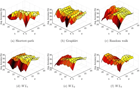
Figure 3 shows a sample of the 10-fold cross validation accuracy (with C =Copt_{) for the}

Laplacian Eigenmap embeddings of the graph kernels on the Shock dataset (see Section 4 for

a description of the dataset), as the number of the nearest neighbours k and the embedding

dimension d vary. While the value of k seems to have a limited impact on the average

classification accuracy, we observe that the optimal performance is achieved for values of d

between 10 and 15. Moreover, note that the optimal value ofd is mostly independent from

both the neighborhood construction and the kernel used. Finally, we should stress that the

selection of an optimal neighborhood size k is a central issue in manifold learning [37]. As

a consequence, the limited impact of k in our framework can be seen as an advantage.

3.2. Graph Kernels

We focus our analysis on four standard graph kernels, namely the shortest-path

(15)

ker-5 10 15 20 5 10 15 20 25 40 45 d k

Avg. Accuracy (%)

(a) Shortest-path 5 10 15 20 5 10 15 20 25 30 35 40 45 d k

Avg. Accuracy (%)

(b) Graphlet 5 10 15 20 5 10 15 20 25 25 30 35 40 d k

Avg. Accuracy (%)

(c) Random walk

5 10 15 20 5 10 15 20 25 25 30 35 40 d k

Avg. Accuracy (%)

(d) W L1

5 10 15 20 5 10 15 20 25 25 30 35 40 d k

Avg. Accuracy (%)

(e) W L2

5 10 15 20 5 10 15 20 25 30 35 40 d k

Avg. Accuracy (%)

[image:15.595.72.528.109.399.2]

(f) W L3

Figure 3: 3D plot of the 10-fold cross validation accuracy (withC=Copt_{) of the graph kernels on the Shock}

dataset as the number of the nearest neighboursk and the embedding dimension dvary. The embedding

was computed using Laplacian Eigenmap.

nel [4]. These are all instances of R-convolution kernels, where the common idea is that of

decomposing two discrete objects and to compare some simpler substructures.

3.2.1. Shortest-path Kernel

LetG= (V, E) be an undirected graph and letS be its shortest-path graph, i.e., a graph

defined over the same set of nodesV where there exist an edge between two nodes if these are

connected by a walk inG. The path kernel counts the numbers of common

shortest-path in two graphs G1 and G2. To this end, the two original graphs are first transformed

into the corresponding shortest-path graphs S1 = (V1, E1) and S2 = (V2, E2). Then, the

shortest-path kernel is defined as

ksp(S1, S2) =

X

e1∈E1 X

e2∈E2

(16)

wherek is a positive definite kernel that measures the similarity between the shortest paths

corresponding to the edges e1 and e2. Moreover, the kernel k can be modified to handle

node labels. In that case, two shortest-path are matched if the sequence of labels along the

two paths are the same.

In their original implementation Borgwardt et al. [1] propose to use the Floyd-Warshall [36]

to compute the shortest-path, yielding a O(|V|4_{) computational complexity.}

3.2.2. Graphlet Kernel

The graphlet kernel measures the similarity between a pair of unlabelled graphs by

counting the number of common graphlets of sizek ={13,4,5} in the two graphs. LetNk

denote the number of graphlets of size k. Given a graphG= (V, E), letfG be the vector of

length Nk where the ith component is the frequency of occurrence of the graphlet gi inG.

For a pair of graphs G1 and G2, the k-graphlet kernel is defined as

kgr(G1, G2) = fG1⊤fG2 (3)

Note that since there are |V_k|

subgraphs of size k in a graph with n nodes, for each graph

the of size |V| the computation of fG has complexity O(|V|k). However, in the case of

graphs with bounded degree d, i.e., graphs where no vertex has more than d neighbours,

the complexity can be shown to be O(|V|dk−1_{). Finally, unlike the shortest-path kernel, the}

graphlet kernel does not take node labels into account.

3.2.3. Random Walk Kernel

The random walk kernel is based on the idea of counting the number of matching walks

between a pair of graphs G1 = (V1, E1) and G2 = (V2, E2). Similarly to the shortest-path

kernel, the random walk kernel can handle node labels. In this work we use the kernel as

defined by G¨artner et al. [13]. To this end, we first introduce the direct product graph

G× = (V×, E×), where V× = {(v1, v2) : v1 ∈ V1, v2 ∈ V2} and E× = {((v1, v2),(w1, w2)) :

(17)

walk kernel betweenG1 and G2 is defined as

krw(G1, G2) =

|V1|

X

i=1

|V2|

X

j=1

∞

X

k=0

µk

Ak

×

ij (4)

where µ is a fixed decay factor that has the effect of reducing the contribution of longer

walks, in addition to allowing the summation to converge. Note that performing a walk

on G× is equivalent to performing simultaneous walks on G1 and G2 [38]. Therefore, the

entries of Ak

× can be seen as the enumerating the simultaneous random walks of length k on G1 and G2. In its original formulation the random walk kernel has computational

complexity O(max(|V1|,|V2|)6), however in [39] a more efficient implementation is proposed

which reduces the complexity toO(max(|V1|,|V2|)3).

One drawback of the random walk kernel is that it is known to be subject totottering [47].

That is, the walker can follow a redundant path h = v1,· · · , vn with vi = vi+2, which can

decrease the ability of the random walk kernel to characterise the graph structure and can

result in an artificially high similarity. For example, the existence of a walk of length 2 can

indicate the presence of a path connecting 3 vertices as well as a walk back and forth along a

single edge. A number of works have proposed to solve the tottering problem by forbidding

repeated visits of the same two nodes [47, 23].

3.2.4. Weisfeiler-Lehman Kernel

The Weisfeiler-Lehman kernel is a state-of-the-art graph kernel introduced by

Sher-vashidze et al. [4]. The kernel enumerates the common subtrees between two graphs by

using the Weisfeiler-Lehman test of graph isomorphism. Given two attributed graphs

G1 = (V1, E1, l1) and G2 = (V2, E2, l2), where li denote the set of labels of Vi, the idea

is that of associating with each vertex v a multiset label based on the labels of the

neigh-bours ofv. This procedure is iterated a fixed number of times, and at each step the resulting

multisets are sorted and compressed to generate new vertex labels. LetGi

1 andGi2 denote the

graphsG1 and G2 afterhiterations of vertices relabeling procedure. The Weisfeiler-Lehman

is then defined as

kh

wl(G1, G2) =

h X

i=0

(18)

wherekδ(Gi1, Gi2) is a positive definite kernel which enumerates the pairs of vertices inGi1 and

Gi

2 that share the same label. The computation of the Weisfeiler-Lehman with h iterations

has complexityO(hm), where m is the number of edges of the graph.

3.3. Manifold Learning

In this paper we investigate the use of four standard non-linear manifold learning

tech-niques, namely Isomap [15], Laplacian Eigenmap [16], Diffusion Maps [17] and Local Linear

Embedding [18]. In the following subsection we assume that we want to embed n points

xi onto an m-dimensional space, with m < n. Note that these techniques can be easily

extended to the case where the input is a pairwise distance matrix rather than a vectorial

representation of the data points. Thus, although graphs are not easily reduced to a

vecto-rial form, it is possible to apply manifold learning to a set of graphs by first computing a

kernel (distance) matrix over the dataset.

3.3.1. Isomap

Isomap can be viewed as an extension of MDS where the original distance between the

points is replaced with their geodesic distance [15]. Isomap assumes that only the pairwise

distances between neighbouring point are known, and uses the shortest-path distance to

estimate the distances between all the other point. More specifically, Isomap starts by

looking for the k-nearest neighbours of each point in the dataset. Then, the k-neigbhours

graph is constructed, where each point is connected with its k-nearest neigbhours. The

geodesic distance between two points is estimated as the shortest-path distance between the

corresponding nodes in the graph. Finally, a low-dimensional projection is generated by

applying MDS on the matrix of geodesic distances.

Despite its popularity, Isomap suffers from a number of drawbacks. In fact, the use of

geodesic distances makes Isomap strongly dependent on the topology of the neighbourhood

(19)

3.3.2. Diffusion Maps

Diffusion Maps attempt to mitigate the shortcomings of Isomap by replacing the geodesic

distances with a more robust distance based on the heat diffusion on the graph [17]. The

first stage requires computing the distance matrix

Mij =e− ||xi−xj||

2σ2 (6)

The matrix M is then normalised to obtain the transition matrix P, such that Pij is the

probability of transitioning fromxi toxj in one time step. The coordinates of theith point

can then be obtained from the eigendecomposition of P as ˜xi = {λ1φi1, λ2φi2, ..., λmφim},

whereP = ΦΛΦT_{, Φ is the} _n_×_n _{matrix Φ = (φ}

1|φ2|...|φn) with the ordered eigenvectors as

columns and Λ = diag(λ1, λ2, ..., λn) is then×ndiagonal matrix with the ordered eigenvalues

as elements.

Note that the matrix P depends on the choice of the time parametert, which until now

we assumed to be equal to 1. However, the diffusion process can be stopped at any a generic

timet ≥1. In this case, Pt

ij gives the probability of transitioning fromi toj int time steps.

In a sense, the Diffusion Map at timet takes into account all the paths of length t between

each pair of points, and for this reason it is extremely robust to noise, as opposed to the

geodesic distance of Isomap.

3.3.3. Laplacian Eigenmap

Similarly to Isomap, the Laplacian Eigenmap method starts by constructing a weighted

graph over the points, where the set of edges connects neighbouring nodes. However, while

Isomap tries to preserve the structure by preserving the geodesic distance, i.e., it tries to

preserve the global structure of the data, Laplacian Eigenmap ensures that points which are

close to each other on the manifold are mapped close to each other in the low-dimensional

embedding space, i.e., it tries to preserve local distances.

LetM denote then×n neighborhood (similarity) matrix for the original points. In

par-ticular, in [16] M is defined as either the Gaussian kernel or the matrix whose element (i, j)

(20)

preserves the distances between neighbouring points is equivalent to solving the generalised

eigenproblem

(∆−M)φi =λiSφi (7)

with eigenvalues λi, eigenvectors φi and ∆ a diagonal matrix whose ith diagonal entry is

∆ii = Pn_j₌₁Mij. Then, the m dimensional embedding is given by the first m eigenvectors

φi, where the eigenvector corresponding to the zero eigenvalues is left out.

3.3.4. Local Linear Embedding

Like Laplacian Eigenmap, Local Linear Embedding is also a local approach that attempts

to preserve the local geometry of each point. The underlying assumption of LLE is that a

point and its neighbours in the original space should lie on or close to a locally linear patch

of the manifold. Hence, it is possible to reconstruct each point as a linear combination

of its neighbours. In particular, the optimal coefficients wij are found by minimising the

reconstruction error

E(W) =

n X

i=1

xi−

X

j∈N(i)

wijxj

!2

(8)

whereN(i) denotes the neighbourhood ofxi.

For each point xi a low-dimensional embedding x˜i is then computed such that the

coor-dinates of each point are still described by the same linear combination of its neighbours.

That is, given the matrix of optimal coefficients W, we look for the set of points x˜i that

minimise the cost function

C(W) =

n X

i=1

˜ xi−

X

j∈N(i)

wij˜xj

!2

(9)

The optimal m-dimensional embedding is then obtained from the m eigenvectors of M =

(I−W)⊤_(I ₋_W_{) corresponding to the} _m _{lowest eigenvalues, where} _I _{denotes the identity} matrix of size n, and the eigenvalues λ0 = 0 and its corresponding eigenvector φ0 are not

(21)

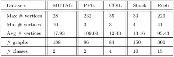
Datasets MUTAG PPIs COIL Shock Reeb

Max # vertices 28 232 35 33 220

Min # vertices 10 3 3 4 41

Avg # vertices 17.93 109.60 12.43 13.16 95.43

# graphs 188 86 84 150 300

[image:21.595.157.438.110.203.2]

# classes 2 2 4 10 15

Table 1: Information on the graph datasets

4. Experimental Results

We perform extensive experiments on 5 different graph datasets (see Table. 1). For

each of the kernels of Subsection 3.2 and the manifold learning techniques reviewed in

Subsection 3.3, we evaluate the class separation before and after computing the embedding

as described in Subection 3.1. More specifically, we first divide the data into a training and

test set. In particular, we assign 80% of the data to the training set and the remaining 20%

to the test set. We repeat the whole procedure 100 times and we report the results in terms

of average classification accuracy,± standard error.

Note that in these experiments we do not include the node labels. In other words, the

kernels consider only the structural information of the graphs. In the case of the

Weisfeiler-Lehman, however, each node is labelled with its degree. Finally, the implementation of the

graphlet kernel used in this paper counts instances of graphlets of size 3.

4.1. Datasets

MUTAG: The MUTAG is a dataset of 188 mutagenic aromatic and heteroaromatic

compounds labelled according to whether or not they have a mutagenic effect on the

Gram-negative bacterium Salmonella typhimurium [40].

PPIs: The PPI dataset consists of protein-protein interaction (PPIs) networks related

to histidine kinase [41]. Histidine kinase is a key protein in the development of signal

transduction. If two proteins have direct (physical) or indirect (functional) association, they

are connected by an edge. Here we consider the PPIs from two different groups: 40 PPIs

(22)

COIL: The COIL dataset consists of 4 objects from the COIL-20 [44] dataset. For each

object, we consider 21 views obtained from equally spaced viewing directions over 105◦. For each image, a graph is obtained as the Delaunay triangulation of the Harris corner points.

Each vertex is used as the seed of a Voronoi region, which expands radially with a constant

speed. The linear collision fronts of the regions delineate the image plane into polygons, and

the Delaunay graph is the region adjacency graph for the Voronoi polygons.

Shock: The Shock dataset consists of graphs from a database of 2D shapes [42]. Each

graph is a skeletal-based representation of the differential structure of the boundary of a 2D

shape. There are 150 graphs divided into 10 classes, each containing 15 graphs.

Reeb: The Reeb dataset consists of a set of adjacency matrices associated to the

com-putation of reeb graphs of 3D shapes [43]. The original 3D shapes dataset comes from the

SHREC database, and consists of 15 classes with 20 shapes each, for a total of 300 objects.

4.2. Experimental Results

Table 2 and Fig. 4 show the average classification accuracy for our approach in the case

where the embedding parameters are chosen so as to maximise the 10-fold cross validation

accuracy on the training set, as explained in Section 3.1. In Fig. 4 the data is displayed as a

series of histograms of the average accuracy. Each individual histogram shows the average

accuracy for the different embedding methods used. The columns of the figure repeat the

histograms for the different kernels studied, and the different rows repeat the histograms

for the different datasets. In Table 2 SP is the shortest-path kernel [1], RW is the random

walk kernel [13], GR is the graphlet kernel [2], while W Lh _{denotes the Weisfeiler-Lehman}

kernel with h iterations [4]. For each kernel and dataset, the best performing manifold

learning technique is highlighted in bold, and the best performing method over the dataset

is underlined. Moreover, for each dataset and each kernel combination, whenever manifold

learning leads to a statistically significant increase or decrease of the performance with

respect to the original kernel the result is highlighted with a∗ symbol.

Our first observation is that the accuracy of the graphlet kernel is consistently higher

(23)

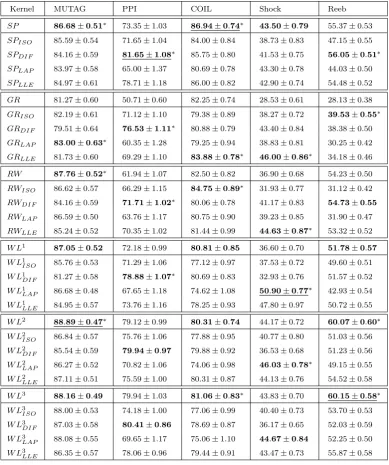
Kernel MUTAG PPI COIL Shock Reeb

SP 86.68±0.51∗ ₇₃_.₃₅_±₁_.₀₃ ₈₆_.₉₄_±₀_.₇₄∗ ₄₃_.₅₀_±₀_.₇₉ ₅₅_.₃₇_±₀_.₅₃ SPISO 85.59±0.54 71.65±1.04 84.00±0.84 38.73±0.83 47.15±0.55

SPDIF 84.16±0.59 81.65±1.08∗ 85.75±0.80 41.53±0.75 56.05±0.51∗

SPLAP 83.97±0.58 65.00±1.37 80.69±0.78 43.30±0.78 44.03±0.50

SPLLE 84.97±0.61 78.71±1.18 86.00±0.82 42.90±0.74 54.48±0.52

GR 81.27±0.60 50.71±0.60 82.25±0.74 28.53±0.61 28.13±0.38

GRISO 82.19±0.61 71.12±1.10 79.38±0.89 38.27±0.72 39.53±0.55∗ GRDIF 79.51±0.64 76.53±1.11∗ 80.88±0.79 43.40±0.84 38.38±0.50

GRLAP 83.00±0.63∗ 60.35±1.28 79.25±0.94 38.83±0.81 30.25±0.42

GRLLE 81.73±0.60 69.29±1.10 83.88±0.78∗ ₄₆_.₀₀_±₀_.₈₆∗ ₃₄_.₁₈_±₀_.₄₆ RW 87.76±0.52∗ 61.94±1.07 82.50±0.82 36.90±0.68 54.23±0.50

RWISO 86.62±0.57 66.29±1.15 84.75±0.89∗ 31.93±0.77 31.12±0.42

RWDIF 84.16±0.59 71.71±1.02∗ 80.06±0.78 41.17±0.83 54.73±0.55

RWLAP 86.59±0.50 63.76±1.17 80.75±0.90 39.23±0.85 31.90±0.47

RWLLE 85.24±0.52 70.35±1.02 81.44±0.99 44.63±0.87∗ 53.32±0.52 W L1

87.05±0.52 72.18±0.99 80.81±0.85 36.60±0.70 51.78±0.57

W L1

ISO 85.76±0.53 71.29±1.06 77.12±0.97 37.53±0.72 49.60±0.51

W L1

DIF 81.27±0.58 78.88±1.07∗ 80.69±0.83 32.93±0.76 51.57±0.52

W L1

LAP 86.68±0.48 67.65±1.18 74.62±1.08 50.90±0.77∗ 42.93±0.54

W L1

LLE 84.95±0.57 73.76±1.16 78.25±0.93 47.80±0.97 50.72±0.55

W L2

88.89±0.47∗ ₇₉_.₁₂_±₀_.₉₉ ₈₀_.₃₁_±₀_.₇₄ ₄₄_.₁₇_±₀_.₇₂ ₆₀_.₀₇_±₀_.₆₀∗ W L2

ISO 86.84±0.57 75.76±1.06 77.88±0.95 40.77±0.80 51.03±0.56

W L2

DIF 85.54±0.59 79.94±0.97 79.88±0.92 36.53±0.68 51.23±0.56

W L2

LAP 86.27±0.52 70.82±1.06 74.06±0.98 46.03±0.78∗ 49.15±0.55

W L2

LLE 87.11±0.51 75.59±1.00 80.31±0.87 44.13±0.76 54.52±0.58

W L3

88.16±0.49 79.94±1.03 81.06±0.83∗ 43.83±0.70 60.15±0.58∗

W L3

ISO 88.00±0.53 74.18±1.00 77.06±0.99 40.40±0.73 53.70±0.53

W L3

DIF 87.03±0.58 80.41±0.86 78.69±0.87 36.17±0.65 52.03±0.59

W L3

LAP 88.08±0.55 69.65±1.17 75.06±1.10 44.67±0.84 52.25±0.50

W L3

[image:23.595.103.493.110.576.2]

LLE 86.35±0.57 78.06±0.96 79.44±0.91 43.47±0.73 55.87±0.58

Table 2: Maximum classification accuracy (±standard error) for the kernels on the graph datasets. For

each kernel and dataset, the best performing manifold learning technique is highlighted in bold, the best

performing method over the dataset is underlined and statistically significant results are marked by a∗.

kernel is significantly higher or equal to that of the original kernel after manifold learning.

Over all the 5 datasets the highest accuracy for this kernel is achieved with the application

of manifold learning. Moreover, the increase in classification accuracy outweighs the loss in

(24)

Sh o rt e st − Pa th G ra p h le t R a n d o m W a lk W − L (h = 1 ) W − L (h = 2 ) W − L (h = 3 ) 7

0 75 80 85 90

NO ML NO ML NO ML NO ML NO ML NO ML ISO ISO ISO ISO ISO ISO DIF DIF DIF DIF DIF DIF LAP LAP LAP LAP LAP LAP LLE LLE LLE LLE LLE MU T AG

Avg. Accuracy (%)

0 50 60 70 80

NO ML NO ML NO ML NO ML NO ML NO ML ISO ISO ISO ISO ISO ISO DIF DIF DIF DIF DIF DIF LAP LAP LAP LAP LAP LAP LLE LLE LLE LLE LLE PPI

Avg. Accuracy (%)

5 70 75 80 85

NO ML NO ML NO ML NO ML NO ML NO ML ISO ISO ISO ISO ISO ISO DIF DIF DIF DIF DIF DIF LAP LAP LAP LAP LAP LAP LLE LLE LLE LLE LLE C O IL

Avg. Accuracy (%)

0 25 30 35 40 45 50

NO ML NO ML NO ML NO ML NO ML NO ML ISO ISO ISO ISO ISO ISO DIF DIF DIF DIF DIF DIF LAP LAP LAP LAP LAP LAP LLE LLE LLE LLE LLE SH O C K

Avg. Accuracy (%)

0 30 40 50 60

NO ML NO ML NO ML NO ML NO ML NO ML ISO ISO ISO ISO ISO ISO DIF DIF DIF DIF DIF DIF LAP LAP LAP LAP LAP LAP LLE LLE LLE LLE LLE R EEB

Avg. Accuracy (%)

[image:24.595.170.735.65.534.2]

(25)

−50 0 50 100 −20

−10 0 10 20 30

(a) Shortest-path

−0.2 −0.1 0 0.1 0.2 0.3

−0.02 −0.01 0 0.01 0.02

(b) Graphlet

−20 −10 0 10 20 30

−4 −2 0 2 4 6

(c) Random walk

−10 −5 0 5 10

−5 0 5 10

(d) W L1

−10 −5 0 5 10

−10 −5 0 5 10 15

(e) W L2

−10 −5 0 5 10 15

[image:25.595.67.528.107.397.2]

(f) W L3

Figure 5: The MDS embeddings of the shortest-path [1], graphlet [2], random walk [3] and

Weisfeiler-Lehman [4] kernels (withh= 1,2,3) on the MUTAG dataset.

the original kernel. Thus, although it is not clear which manifold learning technique should

be preferred, i.e., the optimal technique varies across the 5 datasets, the experimental results

suggest that it is generally a good idea to apply our approach when using a graphlet kernel.

The random walk kernel also seems to benefit from manifold learning, albeit to a lesser

extent. In particular, we observe the best improvement on the PPI and Shock datasets.

However, in contrast to the graphlet kernel, our approach can sometimes lead to a marked

decrease in accuracy, as in the case of the Reeb dataset. The shortest-path kernel and

the Weisfeiler-Lehman kernels show a similar trend, with limited but sometimes significant

improvements. This is the case for the shortest-path kernel on the PPI dataset and the

Weisfeiler-Lehman kernel (h = 1) on the Shock dataset. In general, none of these kernels

shows consistent results in terms of which manifold learning technique to use to enhance

class separation. Interestingly, however, we see that on the PPI datasets each of the kernels

(26)

The above observations seem to support the intuition that those kernels which are based

on the enumeration of small and simple substructures, such as graphlets, are more likely to

suffer from locality problems. The shortest-path and random walk kernels, on the other hand,

utilise larger and more complex structures. The Weisfeiler-Lehman kernel, instead, partially

mitigates the problem by making use of the node labels, which improves node localization

and disambiguation in the evaluation of the kernel. Moreover, to further support our claims,

note that as we increase the value ofhthe benefit of manifold learning becomes less evident.

In fact, by increasing h we are considering subtrees of increasing depth h, thus reducing

locality problems.

Table 2 also shows that the improvement is dataset dependent. We have already noted

that the on the PPI dataset all the kernels benefit from manifold learning, although to

dif-ferent extents. Similarly, we observe statistically significant improvements for the graphlet,

random walk, WL (h = 1,2) kernels on the Shock dataset. By contrast, datasets such as

COIL and MUTAG show little or no improvement. In the case of the COIL dataset, it

is important to note that the structure of the graph is that of a Delaunay graph. Here

the topological information is essentially given by very local structures, i.e., the Delaunay

triangles. As a consequence, the graph structure can be efficiently captured by small and

simple substructures. Hence, we do not observe a substantial improvement or decrease in

performance when manifold learning is applied. More generally, whether or not our

frame-work leads to an increased accuracy ultimately depends on the manifold nature of the data.

Finally, we note that the only kernel that benefits from manifold learning on the MUTAG

dataset is again the graphlet kernel. In fact, as shown in Fig.5, this is the only kernel for

which the MDS embedding shows a clear horseshoe shape.

Table 2 also shows that by unfolding the space through manifold learning we are levelling

to some extent the performances of the examined kernels. This in turn suggests that the

difference between the kernels mainly depends on the level of warping of the embedding

space. This is particularly evident in the PPI and the Shock datasets, where we observe

a marked decrease of the performance gap between the different kernels when manifold

(27)

−1 −0.5 0 0.5 1 −0.5

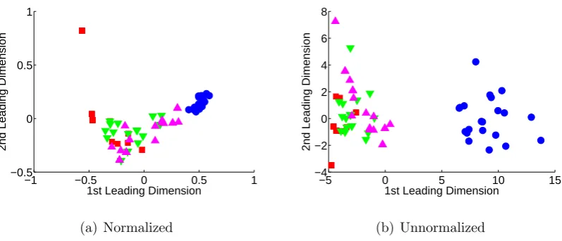
0 0.5 1

(a) Normalized

−5 0 5 10 15

−4 −2 0 2 4 6 8

[image:27.595.100.499.108.279.2]

(b) Unnormalized

Figure 6: The projection of the data from the Hilbert space onto the unit sphere (kernel normalization),

can lead to the formation of horseshoe shaped artifacts.

Finally, we should stress that the gain in accuracy that can be achieved with the proposed

method comes at the cost of an increased computational time. This is due to the need of

exploring the parameter space of Eq. 1 to determine the optimal embedding of the input

graphs. However, note that in general the learning phase is performed only once. Given the

optimal embedding parameters, the classification of the test graphs is straightforward, and

it requires mapping the test graphs to the embedding space, where the classification itself is

performed using a linear kernel.

4.3. Kernel Normalization

A common practice in machine learning is that of normalizing the kernels before the

classification process takes place. More specifically, the kernels are normalized by projecting

the data from the Hilbert space onto the unit sphere. However, note that this can potentially

lead to the formation of horseshoe shaped artifacts, as Fig. 6 shows.

Table 3 and Fig. 7 show the average classification accuracy for our approach in the case

where the kernels are normalized, where in Fig. 7 the data is displayed as a series of

his-tograms of the average accuracy, for eac dataset. If we compare the results in Table 2 with

those in Table 3, we see that the normalized kernels seem to derive more benefits from

manifold learning, when compared to the unnormalized kernels. Note, however, that the

(28)

Kernel MUTAG PPI COIL Shock Reeb

SP 85.08±0.49 69.18±1.00 85.25±0.74 41.03±0.78 55.70±0.50

SPISO 81.95±0.59 75.29±1.15 84.18±0.83 41.80±083 49.30±0.53

SPDIF 84.22±0.57 81.53±1.08∗ 85.87±0.80 41.53±0.75 56.05±0.54

SPLAP 80.35±0.59 69.18±1.12 86.06±0.83 44.40±0.75∗ 47.93±0.82

SPLLE 85.05±0.51 80.00±1.14 83.81±0.85 44.30±0.76 53.50±0.56

GR 82.05±0.56 52.35±0.77 83.81±0.62 31.53±0.62 27.23±0.42

GRISO 82.65±0.57 70.82±1.13 79.63±0.90 40.53±0.74 38.40±0.54

GRDIF 80.51±0.63 76.82±1.12∗ 80.87±0.79 45.03±0.87 38.98±0.50∗

GRLAP 83.81±0.55∗ 64.47±1.17 79.25±0.90 41.07±0.85 29.98±0.52

GRLLE 81.46±0.56 71.52±1.07 83.31±0.78 45.13±0.87∗ ₃₄_.₆₂_±₀_.₄₈

RW 83.86±0.52 64.41±1.00 78.66±0.85 33.90±0.71 25.92±0.41

RWISO 82.76±0.57 70.47±1.08 80.88±0.86 37.80±0.73 29.32±1.79

RWDIF 84.30±0.58 72.29±1.04 80.19±0.77 41.13±0.83 54.75±0.55∗

RWLAP 82.35±0.59 72.05±1.01 75.88±0.96 39.00±0.85 39.47±0.70

RWLLE 82.65±0.57 76.94±1.05∗ 81.12±0.86∗ 43.17±0.84∗ 46.80±0.65 W L1

81.27±0.60 76.76±0.98 79.75±0.91 34.97±0.0.68 33.92±0.42

W L1

ISO 82.51±0.62 71.2±1.03 77.16±1.01 34.76±0.65 44.12±0.54

W L1

DIF 80.84±0.61 78.88±1.07∗ 80.62±0.84 32.93±0.76 51.55±0.52∗

W L1

LAP 83.00±0.61 66.41±1.22 67.56±1.06 44.06±0.86∗ 40.72±0.72

W L1

LLE 84.00±0.58∗ 75.65±1.02 80.56±0.85 43.57±0.77 51.30±0.47

W L2

87.84±0.51∗ ₈₃_.₅₃_±₀_.₈₃∗ ₇₉_.₁₂_±₀_.₈₀ ₃₉_.₁₀_±₀_.₇₂ ₅₀_.₆₀_±₀_.₅₇ W L2

ISO 84.46±0.51 78.71±1.14 76.25±0.97 34.16±0.78 44.85±0.57

W L2

DIF 85.46±0.59 79.94±0.96 79.88±0.92 36.53±0.68 51.25±0.56

W L2

LAP 82.81±0.74 71.59±1.08 73.36±0.97 39.30±0.78 43.03±0.77

W L2

LLE 86.24±0.53 78.35±0.95 77.69±0.89 39.17±0.86 51.83±0.59∗

W L3

86.62±0.55 84.06±0.93∗ 79.01±0.83 40.17±0.70 55.32±0.58∗

W L3

ISO 85.70±0.56 77.47±1.00 74.00±1.00 36.03±0.71 46.5±0.61

W L3

DIF 87.16±0.57∗ 80.41±0.86 78.69±0.87 36.13±0.65 52.03±0.59

W L3

LAP 82.81±0.65 76.59±1.05 71.00±0.98 38.30±0.78 48.87±0.78

W L3

[image:28.595.103.493.109.576.2]

LLE 85.40±0.63 82.30±0.88 79.25±0.96 40.07±0.74 50.57±0.53

Table 3: Maximum classification accuracy (± standard error) for the normalized _{kernels on the graph}

datasets. For each kernel and dataset, the best performing manifold learning technique is highlighted in

bold, the best performing method over the dataset is underlined and statistically significant results are

marked by a∗.

the random walk kernel on the PPI dataset, the accuracy for the normalized kernel with

LLE is significantly higher than any other combination of methods for the unnormalized

(29)

0 75 80 85 90

NO ML NO ML NO ML NO ML NO ML NO ML ISO ISO ISO ISO ISO ISO DIF DIF DIF DIF DIF DIF LAP LAP LAP LAP LAP LAP LLE LLE LLE LLE LLE MU T AG

Avg. Accuracy (%)

0 60 70 80

NO ML NO ML NO ML NO ML NO ML NO ML ISO ISO ISO ISO ISO ISO DIF DIF DIF DIF DIF DIF LAP LAP LAP LAP LAP LAP LLE LLE LLE LLE LLE PPI

Avg. Accuracy (%)

0 65 70 75 80 85

NO ML NO ML NO ML NO ML NO ML NO ML ISO ISO ISO ISO ISO ISO DIF DIF DIF DIF DIF DIF LAP LAP LAP LAP LAP LAP LLE LLE LLE LLE LLE C O IL

Avg. Accuracy (%)

5 30 35 40 45

NO ML NO ML NO ML NO ML NO ML NO ML ISO ISO ISO ISO ISO ISO DIF DIF DIF DIF DIF DIF LAP LAP LAP LAP LAP LAP LLE LLE LLE LLE LLE SH O C K

Avg. Accuracy (%)

0 30 40 50

NO ML NO ML NO ML NO ML NO ML NO ML ISO ISO ISO ISO ISO ISO DIF DIF DIF DIF DIF DIF LAP LAP LAP LAP LAP LAP LLE LLE LLE LLE LLE R EEB

Avg. Accuracy (%)

[image:29.595.160.735.66.534.2]

(30)

the normalization, in some cases applying manifold learning on the normalized kernels

com-pensates for this loss in accuracy. A striking example is that of the random walk and the

Weisfeiler-Lehman (h = 1) kernels on the Reeb dataset, and also to a lesser extent for the

shortest path kernel on PPI. By contrast, in some cases the normalization of the kernel leads

to a better performance, but the accuracy of the kernel remains unaltered when manifold

learning is applied. For example, this is the case of the Weisfeiler-Lehman (h = 1) kernel,

where regardless of the normalization the best accuracy is achieved with diffusion maps.

5. Discussion

Although our experimental evaluation shows that applying manifold learning on the

kernels can enhance class separation, it is not clear which combination of kernel and manifold

learning algorithm leads to the best improvement on a given dataset. In this sense, the

only exception is that of the graphlet kernel, which shows a consistent improvement of the

classification accuracy regardless of the chosen manifold learning technique. In fact, this is

in line with the observation that R-convolution kernels based on the enumeration of small

and simple substructures are more likely to suffer from the locality or ambiguity problems.

This in turn leads to the underestimation of the distances for dissimilar graphs. The result

is to induce a strong curvature on the embedding manifold, which can lead to the manifold

folding over on itself, thus increasing the effective dimensionality of the embedding.

This, in turn, suggests a potential heuristic that can be used to decide when to apply

the proposed approach. Specifically, one may decide to apply manifold learning to a given

dataset and kernel combination after estimating the curvature of the embedding space.

However, this is not a trivial task, since the embedding induced by the kernel is not explicit.

Moreover, one should estimate the local rather than the global curvature. In fact, in our

case measures based on the negative eigenvalues of the distance or dissimilarity matrix such

as the negative eigenratio or the negative eigenfraction [45] commonly used for analysing

the structure of the manifold resulting from the embedding of similarity data fail to detect

any curvature. This is a consequence of the fact that kernels are guaranteed to be positive

(31)

points of high local curvature would be a potential indicator of the type of degeneracies of

the manifold that would benefit from the proposed approach.

Wu, Wilson and Hancock [46] have taken some steps in this direction and have recently

proposed a way to estimate the curvature of a local patch of the manifold, using pairwise

distances between points. Unfortunately, this method works under the assumption that the

neighbours of the point where the curvature is being estimated are uniformly distributed.

This requirement that may not hold on real data, potentially leading to inaccurate

estima-tions. An alternative approach may be to consider the neighborhood of a point and construct

a local kernel. A rapid decay of the eigenvalues of this local kernel would suggest a flat and

low-dimensional embedding space. Conversely, a slow decay of the eigenvalues may suggest

that the point and its neighborhood lie on a subspace of high curvature.

6. Conclusions

In this paper, we have investigated the use of manifold learning techniques on graph

kernels to compute a low-dimensional embedding where the separation of the different classes

is enhanced. We observed that when we perform multidimensional scaling on the distance

matrices extracted from the kernels, the resulting data tends to be clustered along a curve

that wraps around the embedding space, a behaviour that is known to arise when the data

lies on a non-linear manifold. Hence, we proposed to unfold the embedding manifold using

non-linear dimensionality reduction techniques, in an attempt to increase the separation

of the classes. Interestingly, we observed that the unfolding of the space seems level the

performances of the different kernels, suggesting that the existing kernels in the literature

differ mostly in the level of warping of the embedding space. More in general, we observed

that in most of the cases the separation of the data was increased after applying manifold

learning on the original kernels.

Acknowledgments

(32)

References

[1] K. Borgwardt, H. Kriegel, Shortest-path kernels on graphs, in: Proceedings of the Fifth IEEE

Interna-tional Conference on Data Mining, IEEE Computer Society, 2005, pp. 74–81.

[2] N. Shervashidze, S. Vishwanathan, T. Petri, K. Mehlhorn, K. Borgwardt, Efficient graphlet kernels for

large graph comparison, in: Proceedings of the International Workshop on Artificial Intelligence and

Statistics, 2009, pp. 488–495.

[3] H. Kashima, K. Tsuda, A. Inokuchi, in: Proceedings of the 20th International Conference on Machine

Learning, in: ICML, 2003, pp. 321–328.

[4] N. Shervashidze, P. Schweitzer, E. J. van Leeuwen, K. Mehlhorn, K. M. Borgwardt, Weisfeiler-lehman

graph kernels, Journal of Machine Learning Research 12 (2011), pp. 2539–2561.

[5] K. Siddiqi, A. Shokoufandeh, S. Dickinson, S. Zucker, Shock graphs and shape matching, International

Journal of Computer Vision 35 (1) (1999), pp. 13–32.

[6] H. Jeong, B. Tombor, R. Albert, Z. Oltvai, A. Barab´asi, The large-scale organization of metabolic

networks, Nature 407 (6804) (2000), pp. 651–654.

[7] T. Ito, T. Chiba, R. Ozawa, M. Yoshida, M. Hattori, Y. Sakaki, A comprehensive two-hybrid analysis to

explore the yeast protein interactome, Proceedings of the National Academy of Sciences 98 (8) (2001),

pp. 4569.

[8] V. Kalapala, V. Sanwalani, A. Clauset, C. Moore, Scale invariance in road networks. Physical Review

E 73(2) (2006), 026130.

[9] D. Conte, P. Foggia, C. Sansone, M. Vento, Thirty years of graph matching in pattern recognition,

International Journal of Pattern Recognition and Artificial Intelligence 18 (3) (2004), pp. 265–298.

[10] B. Luo, R. C. Wilson, E. R. Hancock, Spectral embedding of graphs, Pattern Recognition 36 (10)

(2003), pp. 2213–2230.

[11] R. C. Wilson, E. R. Hancock, B. Luo, Pattern vectors from algebraic graph theory, IEEE Trans. Pattern

Anal. Mach. Intell. 27 (7) (2005), pp. 1112–1124.

[12] B. Scholkopf, A. J. Smola, Learning with Kernels: Support Vector Machines, Regularization,

Opti-mization, and Beyond, MIT Press, Cambridge, MA, USA, 2001.

[13] T. Gaertner, P. Flach, S. Wrobel, On graph kernels: Hardness results and efficient alternatives, in:

Pro-ceedings of the 16th Annual Conference on Computational Learning Theory and 7th Kernel Workshop,

Springer-Verlag, 2003, pp. 129–143.

[14] D. G. Kendall, Abundance matrices and seriation in archaeology, Probability Theory and Related Fields

17 (2) (1971), pp. 104–112.

[15] J. B. Tenenbaum, V. De Silva, J. C. Langford, A global geometric framework for nonlinear