Spacetime effects on satellite-based quantum communications

(1)

communications

.

White Rose Research Online URL for this paper:

http://eprints.whiterose.ac.uk/81724/

Article:

Bruschi, DE, Ralph, TC, Fuentes, I et al. (2 more authors) (2014) Spacetime effects on

satellite-based quantum communications. Physical Review D - Particles, Fields,

Gravitation, and Cosmology, 90 (4). 045041. ISSN 1550-7998

https://doi.org/10.1103/PhysRevD.90.045041

[email protected] https://eprints.whiterose.ac.uk/ Reuse

Items deposited in White Rose Research Online are protected by copyright, with all rights reserved unless indicated otherwise. They may be downloaded and/or printed for private study, or other acts as permitted by national copyright laws. The publisher or other rights holders may allow further reproduction and re-use of the full text version. This is indicated by the licence information on the White Rose Research Online record for the item.

Takedown

If you consider content in White Rose Research Online to be in breach of UK law, please notify us by

(2)

David Edward Bruschi,1,∗ _{Timothy C. Ralph,}2 _{Ivette Fuentes,}3 _{Thomas Jennewein,}4 _{and Mohsen Razavi}1

1_{School of Electronic and Electrical Engineering,}

University of Leeds, Leeds LS2 9JT, United Kingdom

2_{School of Mathematics and Physics, University of Queensland, Brisbane, Queensland 4072, Australia} 3_{School of Mathematical Sciences, University of Nottingham,}

University Park, Nottingham NG7 2RD, United Kingdom

4_{Institute of Quantum Computing and Department of Physics and Astronomy,}

University of Waterloo, 200 University Avenue West, Waterloo N2L 3G1, Ontario, Canada

(Dated: April 29, 2014)

We investigate the consequences of space-time being curved on space-based quantum communi-cation protocols. We analyze tasks that require either the exchange of single photons in a certain entanglement distribution protocol or beams of light in a continuous-variable quantum key distri-bution scheme. We find that gravity affects the propagation of photons, therefore adding additional noise to the channel for the transmission of information. The effects could be measured with current technology.

PACS numbers:

I. INTRODUCTION

The past century can be regarded as the beginning of the information era. Information science has played a key role in many fields of science, in the development of new technologies and within almost every other hu-man endeavor. At its core, information science aims at understanding how to efficiently encode, transmit, store, manipulate and retrieve information [1]. Although great progress in this field was made considering classi-cal physics alone, in the last decades it was shown that quantum mechanics can bring the game to the next level [2, 3]. With the development of quantum information science, a new wealth of protocols and devices have been proposed and it has been shown that fundamental lim-its valid within the realm of classical physics can now be surpassed [4, 5]. Quantum information science has now been developed up to the point where commercial applications are available. For example, quantum key distribution (QKD) aims at sharing a secret key among two legitimate users, which can be used to achieve se-cure transfer of information. In this work we will ana-lyze quantum communication protocols where the con-sequences of space-time being curved play an important role.

With the turn of the century, several space agen-cies have shown interest in developing and implement-ing quantum communication networks based on tech-nologies such as quantum relays [6]. Several propos-als for quantum communications within low earth orbits (LEOs) have been made, such as the SPACEQUEST and QEYSSAt projects [7–9]. Most proposed systems have

∗_{Current affiliation: Racah Institute of Physics and Quantum}

In-formation Science Centre, the Hebrew University of Jerusalem, Gi-vat Ram, 91904 Jerusalem, Israel

been studied using quantum optics, with little attention given to the theory of relativity, which describers phe-nomena that occur at large scales in the presence of grav-itational fields [8–10]. It is therefore of practical as well as fundamental importance [9] to study such effects on communication protocols when the parties involved (e.g., satellites) are located at great distances within curved space times.

The novel field of relativistic quantum information aims at understanding how relativity affects quantum in-formation tasks [11, 12]. Most of hitherto research has focused on modeling and employing localized systems for quantum information processing [13–15], while only re-cently some attention has been drawn towards under-standing the influence of gravity on quantum protocols. For example, the recent work in [14] shows that when two users employ the modes of quantum fields contained within cavities to perform a teleportation protocol, the motion of one cavity affects the final fidelity of telepor-tation. In [16] it was shown how curvature could effect a large scale photonic interferometer.

In this work we show how gravity affects quantum com-munication protocols and that the effects can be mea-sured with current technology. In particular, we are in-terested in the effects of the Earth’s gravitational field on quantum communications between ground and space links. The main framework that naturally allows to in-vestigate phenomena lying at the intersection of quantum mechanics and relativity is quantum field theory (QFT) [17]. We develop the necessary techniques that allow us to revisit communication protocols between users Alice and Bob located at different heights in a (non uniform) static gravitational potential. In particular, we inves-tigate photon propagation in Schwarzschild space-time, which well approximates the space-time outside non ro-tating spherical planets. We will use quantum optical models for communication generalized to the relativistic QFT scenario like those developed in [18]. However,

(3)

trary to the work in [18], where the main result depends on two observers disagreeing on the notion of particle (mathematically implemented by non-trivial Bogoliubov transformations), in our work, different observers agree on the particle content of a quantum state. For example, a photon created by Alice reaches Bob intact as a single photon. However, we will study how single-photon wave packets exchanged by users are affected by the gravita-tional potential, and how this effect impacts protocols such as entanglement distribution, swapping, or QKD [6]. We show that an Earth-to-space QKD system that relies on entanglement distribution using photons could have an additional contribution to its quantum bit er-ror rate (QBER) of as high as 0.7% as a consequence of space-time curvature. This effect would be observable with current technologies.

We suggest that it is possible to correct for the effects of gravity by employing extra resources. For example, we show that Alice and Bob might use an extra refer-ence beam (a local oscillator) during their communica-tion with Gaussian states. Such extra resources cannot be local but Alice and Bob need to exchange extra in-formation in order to apply the desired corrections. This can, in principle, have a substantial impact on the com-plexity and performance of any quantum communication protocols.

This work is organized as follows. In section II we introduce the tools necessary to address the effects of gravity on quantum communication protocols. In section III we model the creation, propagation on curved back-ground and reception of single photons. In section IV we quantify the effects of curvature on propagating pho-tons. In section V we apply the tools developed in the previous sections to analyze two different quantum com-munication protocols. Finally, in section VI we quantify the effects for realistic configurations. Throughout the paper we take the conventions ~ ₌ _c _{= 1. We use the}

Einstein summation convention i.e., contracted indices are summed over.

II. BACKGROUND TOOLS

In order to study the effects of gravity on quantum communication protocols we will employ tools from QFT and general relativity. On the one hand, QFT provides the description of quantum systems that propagate on a curved but otherwise classical background space-time. On the other hand, general relativity describes the back-ground space-time itself. This standard, but largely ex-perimentally untested approach is referred to as QFT on a curved background [19]. In this section we will provide a the model for the space-time outside a non-rotating planet and the single photons that propagate from the surface to outer space.

A. Space-time outside a planet

The space-time outside a spherical non-rotating body can be modeled by (3 + 1)-dimensional Schwarzschild space-time [20, 21]. Standard Schwarzschild coordinates

xµ_{are (}_{t, r, θ, φ}_{) where}_{t, r}_{represent the proper time and}

radius for observers that are (infinitely) far from the ori-ginr = 0 (also known as the singularity) [20, 21]. The spherical planet responsible for the curvature has mass

M, vanishing angular momentumJ and radiusrE. The

Schwarschild metricgµνin the vacuum outside the planet

is

gµν = diag

−f(r), 1 f(r), r

2_{, r}2_sin_θ

(1)

where f(r) := 1−rs

r, rS := 2GMc2 is the Schwarzschild

radius for the planet andGis the gravitational constant. We assume that the planet’s radius rE is much larger

than its Schwarzschild radius rS, i.e. rE ≫ rS. This

is the case, for example, for the Earth where rS/rE ∼

1.4_×10−9_{. Inside the planet, the metric depends on the} particular model that describes the planet’s matter and its distribution [20]. Since we consider communication outside the planet we are not interested in the space-time forr < rE.

The main effects of gravity for the scenarios of interest in this work will depend on the Schwarschild radiusr. It is well known that field equations with the metric (1) can be solved by separating the solution into temporal, radial and angular part. The full solution to our problem re-quires working with 3 + 1 dimensions and the differential equation for the radial part yield no analytical solution [21]. In contrast, 1 + 1 dimensional Schwarzschild con-tains all of the essential physical properties of its 3 + 1 counterpart, while allowing for simple and analytical for-mulas. We can therefore assume that the problem is es-sentially 1+1 dimensional and that the angular part does not contribute to the effects of interest. This will be rea-sonable provided we only consider radial communication and detector and sources are assumed small compared to

r.The Schwarzschild metricgµν in 1 + 1 dimensions reads

gµν = diag

−f(r), 1 f(r)

. (2)

and the line elementds2_{in Schwarzschild coordinates is}

ds2:=gµνdxµdxν=−f(r)dt2+

1

f(r)dx

2_. ₍₃₎

General relativity predicts that, in the absence of forces, test particles follow geodesics [20]; in 1 + 1 Schwarzschild they coincide with test particles free falling towards the originr= 0. In order to stay at some constant distance from the planet (i.e. r=const) an observer needs to em-ploy some source of acceleration (i.e. a rocket) which counters the gravitational potential. Such trajectory a

(4)

geodesics of constant Schwarzschild radius exist, i.e. cir-cular orbits. In this case no acceleration is needed but the observer must have angular momentum. Satellites for standard communication or the global positioning system (GPS) typically follow such orbits. Furthermore, experi-ments in LEO orbits have recently been proposed to test the effects of gravity on entanglement [22]. In this case, the effects of special relativity, specifically the relative motion of two parties, might contribute to the final ef-fect.

An observer at constant distance r0 from the (center of the) planet employs his or her own clock to measure the time in his or her rest frame. The proper time τ is related to the Schwarzschild time coordinatet by

dτ2 := ds 2

c2

r=r0

=₋f(r0)dt2, (4)

which can be simply integrated to give

τ=pf(r0)t. (5) Equation (5) gives the relation between the proper time

τ of an observer sitting at a constant coordinater0 and the proper timet of an observer (infinitely) far from the planet.

B. Modeling Quantum Optics

In order to study communication protocols that em-ploy the exchange of pulses of light at the quantum level, the optical pulses can be modelled by wave packets built of monochromatic modes (i.e., plane waves) of an un-charged massless scalar field operator Φ(t, x) [17]. It is well known that uncharged scalar fields are a good ap-proximation to the longitudinal (or transverse) modes of the electromagnetic field [14, 17]. The field Φ obeys the standard massless Klein-Gordon equation

Φ = 0, (6)

where the d’Alambertianin curved space times is de-fined as := √1

−g∂µ

√

−g∂µ _and _g _{:= det(}_g

µν). To

solve the Klein-Gordon equation (6) we first notice that every 1 + 1 dimensional space-time is conformally flat [19, 21]. This implies that there always exist coordinates

u=u(t, r), v=v(t, r) such that the Klein Gordon equa-tion (6) takes the form

∂u∂vΦ(u, v) = 0. (7)

In our case, we employ the Eddington-Finkelstein ad-vanced and retarded coordinatesu, v defined by

u := ct₋r_∗

v := ct+r_∗, (8) where the tortoise coordinater_∗ is defined as r_∗ :=r+

rSln|_rr_S −1| [20, 21]. Solutions to the Klein Gordon

equation (7) can be expanded in terms of modes of the form

φ(u)

ω (u) =

eiωu

2√πω

φ(v)

ω (v) =

eiωv

2√πω, (9)

which represent outgoing and ingoing waves that follow geodesicsu=const and v=const, respectively. The fre-quency ω > 0 is the frequency as measured by an ob-server (infinitely) far from the planet with respect to his proper time t. Furthermore, the mode solutions (9) are eigenfunctions of the timelike Killing vectori∂t [19] and

therefore satisfy the eigenvalue equation

i∂tφ(ωu) = ωφ(ωu)

i∂tφ(ωv) = ωφ

(v)

ω . (10)

The mode solutions (9) are normalized through the stan-dard conserved inner product (·,·) (see [17]) by

(φ(u)

ω , φ

(u)

ω′ ) = (φ(_ωv), φ

(v)

ω′ ) =δ(ω−ω′) (11)

while mixed inner products vanish. Finally, the quantum field Φ can be expanded as

Φ =

Z +∞

0

dωhφ(u)

ω aω+φ(ωv)bω+ h.c.

i

, (12)

where the bosonic annihilation operators aω, bω

annihi-late the vacuum state_|0_ithrough the standard relation

aω|0i=bω|0i= 0 and satisfy the canonical commutation

relations

h

aω, a†ω′

i

=hbω, b†ω′

i

=δ(ω₋ω′), (13) where mixed commutators vanish.

III. PREPARATION, PROPAGATION AND

DETECTION OF PHOTONS

We assume ideal optical sources, and will study the propagation on a curved background and how they are affected by such propagation. In particular, we are inter-ested in finding a transformation between the frequency distribution of an optical mode as measured locally be-fore and after propagation.

A. Preparation

In general, a photon can be modeled by a wave packet with a distribution F(ω) _∈ C _{peaked around a central}

frequencyω0 [18, 23]. The annihilation operator for the photon which, for an observer (infinitely) far from the planet, takes the form

aω0(t) =

Z +∞

0

dω e−iωt_F

(5)

The photon creation and annihilation operatorsa†

ω0, aω0

satisfy the canonical equal time bosonic commutation re-lations

aω0(t), a†ω0(t)

= 1 (15)

if the frequency distribution F(ω) is normalized, i.e.

R

ω>0dω|F(ω)|

2_{= 1. Such a distribution naturally arises}

if the optical field is described as a spatially and tem-porally localized propagating physical system [24] i.e., a pulse.

Let Alice and Bob be two observers sitting at different constant distances from the surface of the planet. We can assume that Alice has her laboratory on the surface,

rA=rE, while Bob has his lab on a satellite at constant

distance rB from the surface, rB > rA. Alice and Bob

measure frequencies in their laboratories with respect to

their clocks, i.e., with respect to their proper times τA

and τB. By employing the definition of proper time (5)

and the eigenvalue equation (10), it is simple to show that (10) is equivalent to

i∂τKφ

(u)

ΩK = ΩKφ

(u)

ΩK, (16)

where K=A, B labels Alice or Bob and analogous for-mulas hold for φ(v)_{. In (16), we have introduced the} physical frequency ΩK as measured by the observer at

radiusrK as

ΩK=

ω

p

f(rK)

. (17)

Sinceωtis observer independent, if Alice prepares a sharp frequency mode ΩA, Bob will receive the frequency

ΩB=

s

f(rA)

f(rB)

ΩA, (18)

which is the well known formula for gravitational red-shifts [20]. It is immediate to show that the relation betweenτB and τA is

τB=

s

f(rB)

f(rA)

τA. (19)

In real implementations, special relativistic effects might also affect our systems as satellites might not follow geo-stationary orbits. In this case, satellites will have a veloc-ity component with respect to observers on the ground. It is well known from special relativity that frequencies emitted and received by two observers in relative (uni-form) motion are doppler-shifted.

A more detailed analysis is needed to compute the ex-act impex-act of motion on the shifts in frequency. This would require solving the field equations in at least 2 + 1 dimensions (since satellite orbits lie on a plane). As pointed out before, there are no analytical solutions to the field equations in more than 1+1 dimensions and it is reasonable to assume that the angular component of the

modes would not significantly contribute to the purely gravitational effects we are interested in. The angular part contributes mainly to spreading the beam, an effect which is not of interest here. Nevertheless, we can ex-actly compute, in 3 + 1 dimensions, thetotal relativistic frequency shift between modes emitted by a source and the ones measured by a receiver.

Suppose, the source, Alice, with four-velocity uµ_A, in different dimensionsµ, sends an electromagnetic wave to an observer, Bob, whose four-velocity isvµ_B. We assume that Bob and Alice follow a (different) circular orbit. Let

wν _{be the tangent vector of the null geodesic that the}

light follows. Then the emission frequency ΩA and the

absorption frequency ΩB are related by

ΩB

ΩA

= v

µ_w µ|_B

uµ_w µ|A

,

which can be further simplified using the results in [25] to obtain

ΩB=

v u u

t1−

2M rA

1₋3M rB

ΩA, (20)

which gives the total frequency shift in the 3 + 1 dimen-sional case.

B. Propagation

In order to understand how the propagation of light is affected by the background space-time, we start by noting that Alice or Bob will describe the optical mode (14) through the operator

aΩK,0(τK) =

Z +∞

0

dΩKe−iΩKτKF

(K)

ΩK,0(ΩK)aΩK, (21)

whereK =A, B labels either Alice or Bob, ΩK are the

physical frequencies as measured in their labs using the proper timesτK and ΩK,0are the peak frequencies of the frequency distributionsF_Ω(K_K,)₀. The operators aΩK must

satisfy the canonical commutation relations

[aΩK, a

†

Ω′

K] =δ(ΩK−Ω

′

K). (22)

Our aim in this section is to find the relation between the shape of the wave packetFΩ(AA,)0 prepared by Alice at

some time τA and the shape of the wave packet FΩ(BB,)0

received by Bob at some time τB >

p

f(rB)/f(rA)τA

after propagation through space-time. It is important to notice that Alice’s and Bob’s operators (21) can be used to describe thesameoptical mode in twodifferentframes before and after propagation.

(6)

that at timet > t0 it will be (sharply) localized around

rgiven implicitly by

r∗(r) =r∗(r0) +t. (23)

Equation (23) informs us about at which time Bob will detect photons. On the other hand, equations (18) and (19) inform us of the relation between the frequencies and proper times measured by Alice and those measured by Bob. It is now necessary to find the relation between the operatorsaΩA and aΩB. To do this we employ (13),

(18), (22) and the identityδ(f(x)) =P_iδ(x−xi)

|∂f ∂x||_xi

, where

f(xi) = 0∀i, to write

h

aω, a†ω′

i

= p1

f(r)

h

aΩ, a†Ω′

i

. (24)

This implies thataΩ= 4

p

f(r)aω. Employing all of these

relations, it is now easy to see that the operator (21) can be written before and after propagation as a function of measurable quantities in Alice or Bob’s labs (i.e., peak frequency, bandwidth). Finally, using (14) as an inter-mediate step, we find that the frequency distributions

F_Ω(K_K,)₀ as measured in different reference frames satisfy the relation

F_Ω(B_B,)₀(ΩB) = 4

s

f(rB)

f(rA)

F_Ω(A_A,)₀(

s

f(rB)

f(rA)

ΩB). (25)

Alice can prepare the wave packet aΩA,0(τA) in (21) at

timeτAand send it to Bob who receives it asaΩB,0(τB) at

timeτB>

p

f(rB)/f(rA)τAwhich depends on the user’s

relative distance (i.e., equation (23)). Equation (25) in-forms us that, in general, the wave packet received by Bob will have a different peak frequency and a different shape than those prepared by Alice. In particular, for the scenario of interest where Bob finds himself at higher altitudes than Alice (rB > rA), the wave packet

frequen-cies ΩB as measured by Bob will all be redshifted with

respect to those as created by Alice (see (18)).

Notice that if we wish to take into account the full effects of gravity and motion of the satellite, we find the updated version of (25) as

F_Ω(B_B,)₀(ΩB) = 4

v u u

t1−

2M rA

1₋3M rB

F_Ω(A_A,)₀(

v u u

t1−

2M rA

1₋3M rB

ΩB). (26)

We emphasize that the effect described by (25) can-not be simply corrected by a linear shift of frequencies. Therefore, it may be challenging to compensate the trans-formation induced by the curvature in realistic implemen-tations.

C. Detection

Before leaving Earth to reach his station at heightrB,

Bob agreed with Alice to communicate using light de-scribed by the wave packet F_Ω(A_A,)₀. Let Alice prepare a

pulse described by the mode operator aΩA,0(τA) which

she then sends to Bob who receives it asaΩB,0(τB). We

have shown that, in general, the wave packetF_Ω(B_B,)₀ will

bedifferent compared to the one Bob was expecting. The

difference can be observed in equation (25). Regardless of the specific model of the detector, if the measuring de-vice is tuned to click when a photon in the wave packet

F_Ω(A_A,)₀ is received, the probability of the detector to click

when FΩ(BB,)0 is received will be affected. Bob therefore

will believe that the channel between him and Alice (i.e., the space-time) is noisy. He can quantify the “goodness” of the channel by employing the fidelity_F defined as

F:= Tr2

q_√

ρρ′√_ρ

, (27)

for arbitrary input statesρ, ρ′. In case the input states are pure, for exampleρ=|ψihψ|and ρ′ ₌_|_ψ′_ih_ψ′_|_{, the}

fidelity (27) reduces to _F = _|hψ_|ψ′_i|2 _{and the intensity} fidelity gives the probability that the state wasρ given thatρ′ _{is obtained in a measurement.}

IV. TRANSMISSION AND RECEPTION OF A

SINGLE MODE

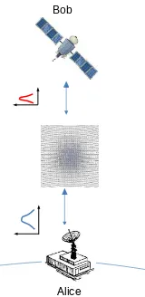
Alice and Bob can communicate using a wealth of pro-tocols [2]. In order to illustrate the techniques developed in the previous section we start with a few simple exam-ples before moving on to more realistic communication schemes. Here we analyze the transmission of a single photon, then the transmission of a coherent state and fi-nally the transmission of a mode which is part of a two mode squeezed state (the scheme is illustrated in figure 1).

A. Single photon

Conceptually, the simplest protocol is when Alice pre-pares a single photon in the modeF_Ω(A_A,)₀ and sends it to Bob. The state_|ψs.p.iof the system at timeτA= 0 is

|ψs.p.i=a†ΩA,0(0)|0i. (28)

Bob now receives the photon

|ψs.p.i=a†ΩB,0(0)|0i, (29)

which is characterized by a distributionF_Ω(B_B,)₀(ΩB)

differ-ent from the distributionF_Ω(A_A,)₀(ΩB) that Alice promised

to send him. The intensity fidelity _F2 _{depends on the} fidelity_Fs.p. of the channel, which in this case is simply the overlap of the two distributions

(7)

Bob

[image:7.612.138.218.59.223.2]

Alice

FIG. 1: Illustration of the setup considered here. Alice and Bob are located at different heights in a gravitational potential. Alice prepares and sends photons (in this work a single photon or a laser beam) to Bob, who uses them to complete a communication protocol. The photon is created by Alice with certain characteristics (i.e., peak frequency and bandwidth), which change once it is received by Bob.

where

∆ :=

Z +∞

0

dΩBFΩ(BB,)0⋆(ΩB)F

(A)

ΩA,0(ΩB). (31)

Clearly ∆ = 1 for a perfect channel. If the curvature is strong enough, the distributions in (31) might have negligible overlap and the fidelity would be low. In the case of Earth-to-LEO communication, we will show that the fidelity (31) is_|∆_|2

∼1₋2_×10−11_.

B. Coherent state

Alice now decides to send Bob a laser pulse instead of a single photon. An initial coherent state _|α_i prepared by Alice with displacementαtakes the form

αi= ˆDA(α)

0i

τ0,A=0

, (32)

where the displacement operator is defined as ˆ

D(α)(τA) := exp(αaΩ†A,0(τA) − α

∗_a_Ω

A,0(τA)). Bob

will receive a coherent state with the same displacement parameter αbut defined for different modesF_Ω(B_B,)₀. The fidelity_Fc.s.in this case will read

Fc.s.=e−2|α|

2₍₁

−ℜ(∆))_, ₍₃₃₎ where_ℜ(∆) denotes the real part of ∆.

C. Two mode squeezed state

As a last case Alice will send Bob one mode of two mode squeezed state|si. The state|sitakes the form

si= ˆSA(α)

0i

τ0,A=0

, (34)

where thesqueezing operator is defined as

ˆ

S(s)(τA) :=e s

a†Ω_A,₀(τA)b†_Ω′

A,0

(τA)−aΩA,0(τA)bΩ′_A,₀(τA)

andsis known as the squeezing parameter [23, 26]. We assume that Alice has prepared the modebΩ′

A,0(τA) which

is received as modeb′

Ω′

B,0(τB) by Bob. In this scenario,

an operational definition of fidelity involves comparing the state _|s_i that Bob and Alice expect to share with the state_|s_i′ _{they actually share after the propagation of}

modebΩ′

A,0. The fidelity computed this way sets a lower

bound to the average fidelity of communication between Alice and Bob. The state _|s_i′ _{takes the form (34) with} b′

Ω′

A,0 in place ofbΩ ′

A,0. We can compute the fidelityFt.s.

for this scenario asFt.s.=|hs|si′|and we obtain

Ft.s. =

1 cosh2s

1 1₋∆ tanh2s

2

. (35)

Note that, no matter how well the modes overlap (i.e., how small is 1_{− |}∆_|) as long as the overlap is not perfect the fidelity (35) vanishes for infinite squeezing.

V. COMMUNICATION BETWEEN DIFFERENT

ALTITUDES (OR COMMUNICATION IN A GRAVITATIONAL POTENTIAL)

A. Establishing entangled links for communication protocols

(8)

Bob

Alice

SPS QM - A

D1 D2

SPS QM - B

50:50 BS

BS

BS b

a

a',d' b'

̃ a ,c̃ ̃ b ,d̃

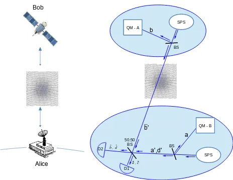
FIG. 2: (Color online) Schematic diagram for entanglement distribution between two quantum memories (QMs) located at Alice’s and Bob’s locations. Single photon sources (SPSs), memories and detectors are represented by circles, squares and half-circles, respectively. Vertical bars denote beam split-ters. In this protocol, the detection of a single photon after a beam splitter ideally projects the two memories onto an entangled state.

1. Flat space-time entangling protocol

We briefly describe the ideal flat space-time setup em-ployed by our users. The scheme that Alice and Bob will use is depicted in Fig. 2. Alice and Bob have a quantum memory and a single photon source each. The single photon sources produce one photon each, which travel through two balanced (for simplicity) beam splitters lo-cated at the respective stations, as shown in Fig. 2. The photons are either transmitted (modes a′_b′_{) or are}

re-flected and are then stored in the memory (modes a, b). The stateΨiniof the system at this point of the scheme is

Ψini= 1

2



1100

| {z }

aba′_b′

i+0110i+1001i+0011i 

. (36)

The modes a′_{, b}′ _{are then recombined at a second}

bal-anced beam splitter located at the Alice’s station and the output modes ˜a,˜b are measured. Here, we assumed the phase difference between the two paths is fixed and compensated. Time synchronization is also in place to ensure that the photons arrive at the same time at the beam splitter of the measurement module. Note that the overall phase of the initial single photons does not affect the final state obtained and no coordination is needed to drive both single-photon sources coherently.

To understand what is the action of the detection process we start by writing the transformation between

modesa′_{, b}′ _{and modes ˜}_a,˜_b_as

˜

a

˜_b

= √1

2

1 1 1 ₋1

a′ b′

. (37)

If modes ˜a or ˜b are detected, i.e. detectors D1 or D2 click, the state of the memories is projected respectively into

ρ_±= 1 2P±+

1

2Pvac. (38)

whereP± denote projectors on the maximally entangled

states

Ψ_±i=√1

2

10

|{z}

ab

i ±01i, (39)

whilePvac. denotes the projection on the vacuum state. In case number resolving photodetectors are employed, we can exclude the cases when two photons arrive at the same detector and therefore ideallyΨouti=Ψ_±i, with

|φ_i+₍

|φ_i−_{) heralded by a click at D1 (D2). Note that}

there is still a chance that one of the two photons is lost along the way, therefore degrading the state. For the sake of our argument, in this work we are not interested in any source of loss or imperfection and from now on we will assume that detectors are ideal and photons always reach their destination.

2. Curved spacetime entangling protocol

The scheme described above works when Alice and Bob are in flat space-time. Let Alice and Bob now be in curved Schwarzschild space-time in the same setup as described in the previous section and depicted in fig-ure 2. We assume for simplicity that Alice’s modes act as reference modes, since it is much more feasible that all operations of interest occur at her station. In case the operations were performed between Alice and Bob or at Bob’s station, the results would be qualitatively the same. Bob will generate a photon in modeb′ _{which will}

enter the beam splitter on Earth as a different mode ¯b′

than the expected one. Therefore, we can decompose the mode ¯b′ _{that reaches Earth as}

¯_b′ ₌p₁₋_{q b}′₊√_{q c}′_, ₍₄₀₎

whereq≤1. Equation (40) states that when Bob’s mode reaches the Earth, it will have a contribution from mode

b′ _{(which matches Alice’s mode} _a′_{) and a contribution}

from the orthogonal mode c′_{, i.e. [}_a′_{, c}′†_{] = 0. Such a}

decomposition is always possible [35].

The parameter q is directly related to the fidelity of single photon transmission as defined in (31). In fact,

∆ =h0¯b′b′†0i=p1−q, (41) which implies

[image:8.612.67.299.57.236.2]

(9)

We can assume without loss of generality that ∆∈R_{. It}

is straightforward to generalize all of the following results to the case of complex ∆.

The balanced beam splitter will mix mode a′ _with _b′

and modec′_{with a corresponding mode}_d′_{. Both couples}

are transformed to new outputs ˜a,˜band ˜c,d˜respectively

by a transformation of the form (37). Notice that since all operations occur at Alice’s station, the moded′_{is always}

in its ground state. The initial stateΨini of the whole

system before modesa′_b′_c′_d′ _{enter the beam splitter on}

Earth is

Ψini=1

2



110000 | {z }

aba′_b′_c′_d′

i+011000i+p1−q100100i+√q100010i+√q001100i+p1−q001010i 

. (43)

We can now invert the relation between a′_{, b}′ _{and ˜}_a,˜_b (analogously for the second couple of modes) and ex-press the state (43) in terms of memory modes a, b and the beam splitter output modes ˜a,˜b,˜c,d˜. The expression involves fifteen terms and is not illuminating. The Bell state measurement on Earth is completed when the pho-todetectors absorb the photons. If detector D1 clicks, modes ˜aand ˜chave been detected. The projection oper-ator that implements this detection is

D+=1a,b⊗Nˆ ⊗ |0ih0| ⊗Nˆ ⊗ |0ih0|, (44)

where ˆN := 1− |0ih0| and the order of the modes is

a, b,˜a,˜b,c,˜d˜. If detector D2 clicks, this corresponds to projecting the initial state Ψini with the operator D−

of the form

D−=1a,b⊗ |0ih0| ⊗Nˆ⊗ |0ih0| ⊗N .ˆ (45)

The final states

ρ_±(q) :=Trphot.[D±|ΨinihΨin|] Tr[D±|ΨinihΨin|]

(46)

of the memories, after detection and absorption of single photons by the resolving photodetectors, are respectively

ρ± =1₂

h

(1±p1−q)P++ (1∓

p

1−q)P−

i

. (47)

In equation (47),P±represents the projector on the state

|Ψ_±_i. Sinceρ_±(q) is a mixed state, we can compute the NegativityN which is a measure of entanglement based on the positivity of the partial transpose (PPT criterion) [36, 37]. In order to compute the negativity we first need to find the partial transpose ρPT

± of the state ρ±. This

can be obtained by transposing the subspace of one of the two modes. Then, we define

N[ρPT_± ] := max

(

0,X

i

|λi| −λi

2

)

, (48)

where λi are the eigenvalues of the partial transposed

stateρPT

± . In our scenario it is easy to show that

N =

√

1−q

2 . (49)

The Negativity reaches the value_N = 1/2 for maximally entangled states. It is easy to see from (40) that when

q= 0 the mode sent by Bob reaches Alice intact (i.e., cen-ter and shape of the frequency distribution is unchanged) and therefore the memories are projected into a maxi-mally entangled state as expected (see (47)).

B. A simple continuous-variable QKD protocol

As an instructive counter example we now consider a type of quantum communication protocol whose perfor-mance is not affected by curvature. While some proto-cols require the users to perform only local operations and exchange quantum systems, other protocols require the users to exchange additional systems, such as local oscillators. The latter systems might naturally incorpo-rate the means for the compensation of the effects due to space-time curvature. Here, we will use the techniques developed above to analyze one such example of a contin-uous variable QKD protocol similar to that investigated in [18]. Alice employs two coherent states originating from the same source (i.e. a laser) with strong power. The source is then split up into one strong beam which is used as a reference (the Local Oscillator) and one weak beam used as a signal. Bob collects the two beams, mixes them at a balanced beam splitter and measures the pho-tocurrents of the two output modes. In this section we will show that by using extra resources (i.e., the Local Oscillator) Bob will be able to compensate for the effects of the curvature of space-time.

Let Alice prepare the signal and the LO initially in two different coherent states_|α_iand _|β_i of modesaS,A,aL,A with displacement parameters that satisfyβ ≫ |α|. Since the modes come from the same source, they have the same frequency distribution (_FΩL,A =FΩS,A = FΩ0,A).

A coherent state is obtained by acting with the displace-ment operator ˆD(γ) = exp(γˆa†₋_γ∗_ˆ_a_{) on the vacuum}

state |0i. The initial state for this kind of protocol is therefore

ψii= ˆDS,A(α) ˆDL,A(β)

0i

τ0,A=0

(10)

where the subscripts S, L denote the signal or the lo-cal oscillator and subscriptsA, B the user that prepares and/or receives it. The modesaS,A and aL,A propagate and reach Bob, who mixes them at a balanced beam split-ter described by the transformation (37). We know that the modes received by Bob aredifferent from the modes sent by Alice, i.e., the peak frequency and the width of the distributions are different as measured by Alice and Bob. Bob will perform a measurement, i.e., count incident photons, for some time much longer than the bandwidths considered in this problem (see [18]). There-fore, he will integrate the input signals of his detectors over an infinite (proper) time. The operator that de-scribes the outcomes of balanced homodyne detection at Bob’s satellite (and with respect tohis reference frame) is [18, 23, 26]

ˆ

O:=

Z +∞

−∞ dτB

h

ˆ

a†_S,B(τB)ˆaL,B(τB) + h.c.

i

. (51)

Bob will compute the expectation value of such operator using the stateψiihe receives. We are interested in the

final expectation valueX :=_hψi

Oˆψii. In order to

com-pute the observable X we follow [18] and assume that the detector is well localized in space and time. This implies that it responds with the same strength to a very broad range of frequencies, therefore ˆaL,B(τB) and ˆaS,B(τB) are

broadband. We can commute the displacement operators through the mode operators as expressed in Bob’s coor-dinates to give the following relations at Bob’s site [18]

ˆ

D†_L,B(β)ˆaL,B(τB) ˆDL,B(β) =

ˆ

aL,B(τB) +

β

√

2πΩ0

Z +∞

0

dΩBe−iΩBτBFΩ0,B(ΩB)

ˆ

D†_S,B(α)ˆaS,B(τB) ˆDS,B(α) =

ˆ

aS,B(τB) +

α

√

2πΩ0

Z +∞

0

dΩBe−iΩBτBFΩ0,B(ΩB)

, (52)

where the signal/local oscillator modes he receives have the same frequency distribution_FΩ0,B as previously

dis-cussed. Using the relations (52) we obtainX

X = β[α∗+α]. (53)

Another quantity of interest is the varianceV of this ex-pectation value defined as [18, 23, 26]V :=_hψi

Oˆ2ψii −

(_hψi

Oˆψii)2. We can compute the varianceV and find

V = 2 _|β_|2+_|α_|2_∼2_|β_|2 (54)

sinceβ_{≫ |}α_|.

The result of the homodyne detection (53) and its vari-ance (54)are not affected by the space-time curvature. One way to understand this conclusion is that Alice sends Bob a signal, which will change its frequency distribution profile, and a LO, which will be affected in the same way. Bob will use the LO as a reference beam for matching and detection of the input signal. Therefore, the effects of the change in frequency profile are compensated. We conclude that the key rate of any protocol using such quantum communication scheme will not be affected.

VI. ESTIMATION OF EFFECTS OF SPACE-TIME CURVATURE ON EARTH-TO-LEO

QUANTUM COMMUNICATION IMPLEMENTATIONS

There has been extensive research on expanding the distances of quantum communications and QKD. For ground based systems, the hard limit is optical losses in fibers and free-space, which scales exponentially with distance [2]. Quantum Repeaters are one way to extend distances on the ground, however there are still many fundamental challenges to be researched before they can be practical [32]. Satellite transmissions solve this prob-lem, because the transmission losses in empty space scale only quadratically with the distance. With todays tech-nologies, distances of up to 100,000 km are feasible in empty space.

(11)

the Chinese Academy of Science, which has announced openly that it is investigating the possibility of perform-ing quantum communications in space (launch date of 2016) [41].

The growing interest in developing and implementing efficient quantum networks in space motivates the esti-mation of all possible effects that can influence the reli-ability of the networks and jeopardize the missions. We have shown that entanglement distribution between users at different heights in a gravitational potential is affected by the curvature. Here, we numerically look at such effects on current and future quantum communication technologies. It turns out that current regimes of opera-tions for proposed satellite are based on technologies that are weakly affected by gravity. However, next-generation satellite missions may implement technologies that are based on narrowband optical systems which could expe-rience substantial and measurable effects.

In this section we focus on regimes of operation in which the impact of space-time curvature on quantum communication protocols is significant. Suitable can-didates for a single photon source are cavity-enhanced spontaneous parametric down-conversion sources (cavity enhanced SPDCs) or atomic-vapor based single photon sources [42–45]. The regime of operation of interest, ac-cessible by the current technology, is for center wave-lengts of Ω0 = 428 nm or shorter and bandwidths of

σ = 1MHz or lower, where σ ≪ Ω0. While this length is significantly shorter than the the typical wave-lengths for conventional optical sources, ranging from 780 nm (384 THz) to 1550 nm (193 THz) [46], it will be fa-vorable for long distance free space transmission due to its low diffraction induced loss [47].

A. Gaussian wave packets

Let Alice and Bob employ single photon sources with such features. The normalized wave packets at both sta-tions will have the form

FΩ0(Ω) =

1

4

√

2πσ2e

−(Ω−₄_σΩ0)2 2_, ₍₅₅₎

where we have assumed the wave packet is real without loss of generality. As discussed in the previous section, the propagation of one photon in the gravitational field from Alice’s station to Bob’s station (or viceversa) will affect the shape of the photon’s wave packet. In particu-lar, if the photon was sent by Bob with wave packetF_Ω(B_B,)₀

of the form (55), it will be received by Alice as a photon with a wave packetFΩ(AA,)0 that differs to the original one

and is related toF_Ω(B_B,)₀ by (26).

We have shown that the mode overlap ∆ quantifies the effects of gravity on the entanglement distribution, when photons are sent by one user and processed at a different location. In the case of the protocol considered in section V, we need to compute ∆ at Alice’s station and express

the Negativity N as a function of ∆ through (49) and (42). We find

∆ =

Z +∞

−∞ dΩAF

(A) ΩA,0(ΩA)F

(B)

ΩB,0(ΩA). (56)

Note that the integral should be performed over stricly positive frequencies. However, since Ω0 _≫σ, it is possi-ble to include negative frequencies without affecting the value of ∆. Using (55) and (26), simple algebra allows us to conclude that in our case

∆ =

s

2(1_±δ) 1 + (1±δ)2e

− δ2 Ω2B,0

4(1+(1±δ)2 )σ2, (57)

where we have defined

δ=

4

v u u

t1−

2M rA

1−3M rB

−1

(58)

and the signs± occur for rB < rA or rB > rA

respec-tively. Notice that δ = 0 occurs either when Alice and Bob are in flat space-time (f(rA) =f(rB) = 1) or Alice

and Bob are at the same height (f(rA) =f(rB)). In both

cases the modes perfectly overlap (∆ = 1) as expected and there is no effect due to gravity.

Combining equation (57) with (49) we can predict how any protocol that depends explicitly on the mode overlap ∆, for example the entanglement distribution protocol of section V, is affected by the space-time channel. We can use typical values for Earth to LEO communication and set rA = 6371km and rB = 6771km (i.e. the ISS orbit

of about 400km). Since the Schwarzschild radius of the Earth isrS = 9mm, we find that

δ_{∼ −}1

4(

rs

rB −

rs

rA

) = 1.45_×10−11_. ₍₅₉₎ We notice from (57) that two different scenarios can oc-cur.

i) If δΩB,0

σ ≤δ≪1 then

∆∼1− O(δ2), (60)

and therefore it is easy to see thatq_∼δ2

≤10−20_. In this case the effects are independent of the peak frequency and on the width of the distribution and are negligible.

ii) Surprisingly another scenario is possible, whenδ_≪

(δΩB,0 σ )

2

≪ 1, which occurs for typical communi-cation where ΩB,0 = 700THz (corresponding to a wavelength of about 420 nm) andσ= 1MHz. For example, similar peak frequency and bandwidths have been achieved by trapped ion experiments [48]. Then

∆∼1−δ

2_Ω2

B,0

8σ2 = 1.3×10−

(12)

and thereforeq∼(δΩB,0

2σ )

2_{= 2}_.₆_×₁₀−3_{. This effect} is much larger than the one in the previous scenario and very close to the threshold of measurable effects with current technology. Furthermore, if Bob were to be very far from Earth (f(rB) = 1) then we

would have δ= 3.5×10−10_{. With the same pulse} characteristics we would achieve q _∼ (δΩB,0

2σ )

2 ₌

1.5×10−2 _{which would be a 0}_._{7% correction to the} ideal Negativity _N = 1/2 of flat space-time. This would produce measurable effect in the QBER of QKD protocols [49].

We can evaluate the effects of curvature on entan-glement distribution for different types of sources. If Bob employed a Rb vapor type source with ΩB,0 ∼ 380THz and σ ∼ 5MHz we find q ∼ 2.52_×10−4_{, while for NV centres the effect is even} smaller,q∼10−6.

B. Impact on realistic communication protocols

Two users Alice and Bob can employ QKD protocols to share a secret key. We assume that the users do not need to trust any node , source or device that is employed (device independent QKD). A relevant figure of merit for a QKD protocol is given by the QBER, defined as the ratio of exchanged error bits and the total number of sifted key bits. Using the entanglement distribution scheme of Fig. 2, Alice and Bob can employ the QKD protocol proposed in [6] to share secret keys. Under the same assumptions as in section V A 1, in Appendix A we show that for such a protocol theQBER∼ q

2 which implies

QBER_∼δ 2_Ω2

B,0

8σ2 (62)

which can reach the value_∼0.7% for Ω0 = 480nm and

σ= 1MHz. This could be a noticeable effect in realistic implementations of QKD, which typically operate with QBERs of a few percent [49].

Equation (62) accounts for effects due to only the cur-vature of space-time. The QBER that would be mea-sured in realistic experiments must take into account other sources of errors, such as dark counts, channel losses, detector and sources imperfections, flatness across the spectrum of all devices (sources, beam splitters, de-tectors).

VII. CONCLUSIONS

We have introduced mathematical techniques to study and quantify the effects of gravity on quantum informa-tion and quantum communicainforma-tion protocols. We have shown that photon propagation is affected by the curva-ture of space-time, and may change their frequency dis-tribution in centre, shape and bandwidth. We analyzed

two different protocols, an entanglement distribution pro-tocol and a continuous variable QKD propro-tocol. We have shown that communications between two users that are located at different heights in the gravitational potential of the Earth are affected by the curvature of the space-time. Our results identify additional effects which cannot occur if two parties are situated at the same height or are in flat space-time. Therefore, the results of this paper unveil that there exist effects of gravity on quantum in-formation protocols that cannot be reproduced and stud-ied in Earth-based laboratories. These curvature effects would occur in addition to those due to special relativity or noise.

While typical predictions of quantum field theory, such as the Dynamical Casimir effect, require enormous accel-erations [50], the effects studied in this paper are there-fore relevant for possible space based implementations of satellite missions based on current technologies and could potentially be tested within near-future proposals for satellite missions. While these effects could in princi-ple be compensated by exchange of additional resources (use of local oscillators, tunable receiving devices, tun-able sources), they will help us to investigate the overlap between quantum mechanics and the theory of general relativity.

Acknowledgements

We thank Daniel K. Oi, Jason Doukas, Mehdi Ah-madi, Nicolai Friis, Antony Lee, Jorma Louko and Paolo Villoresi for useful discussions and comments. This work was in part supported by the UK Engineering and Physical Science Research Council grant number EP/J005762/1 and the European Community’s Seventh Framework Programme under Grant Agreement 277110. T. Jennewein acknowledges support from NSERC, CI-FAR, CFI, the Ontario Ministry for Science, Indus-try Canada, CSA. D. Bruschi would like to thank the university of Nottingham for hospitality. I. Fuentes acknowledges support from EPSRC (CAF Grant No. EP/G00496X/2).

Appendix A: QBER

We apply our results to a well known scheme such as the one described in [6]. There, Alice and Bob have two memories each, A, A′ _and _{B, B}′ _{respectively. They use}

the scheme in Section V A 2 to entangle A with B and

A′_with_B′_{. The modes stored in the memories}_{A, A}′ _can

then be mixed at a balanced beamsplitter, and analo-gously for the modes in memoriesB, B′_{. If one detector}

(13)

same (i.e., bothρ+ orρ−). This occurs on average with

probability pshare = (1−

√

1−q)2

4 +

(1+√1−q)2

4 . The proba-bility of Alice and Bob not sharing the same bit is instead

pdiff= 2(1+

√₁ −q) 2

(1−√1−q) 2 .

The QBER is defined as the number of different bits shared by Alice and Bob over the total bits exchanged,

namely QBER:= _psharepdiff₊_pdiff. Substituting forpshare and

pdiff we find

QBER = q 2.

[1] C. E. Shannon, Bell System Technical Journal 27, 379 (1948).

[2] V. Scarani, H. Bechmann-Pasquinucci, N. J. Cerf, M. Duˇsek, N. L¨utkenhaus, and M. Peev, Rev. Mod. Phys.

81, 1301 (2009), URL http://link.aps.org/doi/10. 1103/RevModPhys.81.1301.

[3] R. Alleaume, J. Bouda, C. Branciard, T. De-buisschert, M. Dianati, N. Gisin, M. Godfrey, P. Grangier, T. Langer, A. Leverrier, et al. (2007), arXiv:0701168v1 [quant-ph], URL http://arxiv.org/ abs/quant-ph/0701168.

[4] C. H. Bennett and G. Brassard, in Proceedings of the IEEE International Conference on Computers, Systems and Signal Processing(IEEE Press, New York, 1984), pp. 175–179.

[5] P. W. Shor, inFoundations of Computer Science, 1994 Proceedings., 35th Annual Symposium on (1994), pp. 124–134.

[6] L. M. Duan, M. D. Lukin, J. I. Cirac, and P. Zoller, Nature414, 413 (2001), URLhttp://dx.doi.org/10. 1038/35106500.

[7] J. M. Perdigues Armengol, B. Furch, C. Jacinto de Matos, O. Minster, L. Cacciapuoti, M. Pfennigbauer, M. Aspelmeyer, T. Jennewein, R. Ursin, T. Schmitt-Manderbach, et al., Acta Astronautica63, 165 (2008). [8] Ursin, R., Jennewein, T., Kofler, J., Perdigues, J. M.,

Cacciapuoti, L., de Matos, C. J., Aspelmeyer, M., Valen-cia, A., Scheidl, T., Acin, A., et al., Europhysics News

40, 26 (2009), URL http://dx.doi.org/10.1051/epn/ 2009503.

[9] D. Rideout, T. Jennewein, G. Amelino-Camelia, T. F. Demarie, B. L. Higgins, A. Kempf, A. Kent, R. Laflamme, X. Ma, R. B. Mann, et al., Classical and Quantum Gravity 29, 224011 (2012), URL http: //stacks.iop.org/0264-9381/29/i=22/a=224011. [10] M. Zych, F. Costa, I. Pikovski, and C. Brukner, Nat.

Comm. 2, 505 (2011), URL http://dx.doi.org/10. 1038/ncomms1498.

[11] T. C. Ralph and T. G. Downes, Contemporary Physics

53, 1 (2012).

[12] P. M. Alsing and I. Fuentes, Classical and Quantum Gravity 29, 224001 (2012), URL http://stacks.iop. org/0264-9381/29/i=22/a=224001.

[13] D. E. Bruschi, I. Fuentes, and J. Louko, Phys. Rev. D

85, 061701 (2012), URLhttp://link.aps.org/doi/10. 1103/PhysRevD.85.061701.

[14] N. Friis, A. R. Lee, K. Truong, C. Sab´ın, E. Solano, G. Johansson, and I. Fuentes, Phys. Rev. Lett. 110, 113602 (2013), URL http://link.aps.org/doi/10. 1103/PhysRevLett.110.113602.

[15] N. Friis, M. Huber, I. Fuentes, and D. E. Bruschi, Phys. Rev. D86, 105003 (2012), URLhttp://link.aps.org/ doi/10.1103/PhysRevD.86.105003.

[16] M. Zych, F. Costa, I. Pikovski, T. C. Ralph, and ˇ

C. Brukner, Classical and Quantum Gravity29, 224010 (2012), URLhttp://stacks.iop.org/0264-9381/29/i= 22/a=224010.

[17] M. Srednicki, Quantum Field Theory (Cambridge Uni-versity Press, 2007).

[18] T. G. Downes, T. C. Ralph, and N. Walk, Phys. Rev. A

87, 012327 (2013), URLhttp://link.aps.org/doi/10. 1103/PhysRevA.87.012327.

[19] N. D. Birrell and P. C. W. Davies, Quantum Fields in Curved Space, Cambridge Monographs on Mathematical Physics (Cambridge University Press, 1900?).

[20] C. W. Misner, K. S. Thorne, and J. A. Wheeler, Gravi-tation (W. H. Freeman, 1973).

[21] R. M. Wald, General Relativity (University of Chicago Press, 1984).

[22] D. E. Bruschi, C. Sab´ın, A. White, V. Baccetti, D. K. L. Oi, and I. Fuentes (2013), quant-ph/1306.1933, URL

http://arxiv.org/abs/1306.1933.

[23] U. Leonhardt, Measuring the Quantum State of Light, Cambridge Studies in Modern Optics (Cambridge Uni-versity Press, 2005).

[24] D. E. Bruschi, A. R. Lee, and I. Fuentes, Journal of Physics A: Mathematical and Theoretical 46, 165303 (2013), URLhttp://stacks.iop.org/1751-8121/46/i= 16/a=165303.

[25] L. Hodgkinson, Ph.D. thesis, School of Mathemati-cal Sciences (2013), URLhttp://arxiv.org/pdf/1309. 7281v2.pdf.

[26] M. O. Scully and M. S. Zubairy,Quantum Optics (Cam-bridge University Press, 2002).

[27] A. K. Ekert, Phys. Rev. Lett.67, 661 (1991), URLhttp: //link.aps.org/doi/10.1103/PhysRevLett.67.661. [28] C. H. Bennett, G. Brassard, and N. D. Mermin, Phys.

Rev. Lett.68, 557 (1992), URLhttp://link.aps.org/ doi/10.1103/PhysRevLett.68.557.

[29] C. H. Bennett, G. Brassard, C. Cr´epeau, R. Jozsa, A. Peres, and W. K. Wootters, Phys. Rev. Lett. 70, 1895 (1993), URLhttp://link.aps.org/doi/10.1103/ PhysRevLett.70.1895.

[30] M. Razavi and J. H. Shapiro, Phys. Rev. A 73, 042303 (2006), URL http://link.aps.org/doi/10. 1103/PhysRevA.73.042303.

[31] N. Sangouard, C. Simon, J. c. v. Min´aˇr, H. Zbinden, H. de Riedmatten, and N. Gisin, Phys. Rev. A

76, 050301 (2007), URLhttp://link.aps.org/doi/10. 1103/PhysRevA.76.050301.

[32] N. Sangouard, C. Simon, H. de Riedmatten, and N. Gisin, Rev. Mod. Phys.83, 33 (2011).

[33] H.-K. Lo, M. Curty, and B. Qi, Phys. Rev. Lett.

108, 130503 (2012), URL http://link.aps.org/doi/ 10.1103/PhysRevLett.108.130503.

(14)

[35] P. P. Rohde, W. Mauerer, and W. Silberhorn, New Jour-nal of Physics 9, 91 (2007), URL http://stacks.iop. org/1367-2630/9/i=4/a=091.

[36] A. Peres, Phys. Rev. Lett.77, 1413 (1996), URLhttp: //link.aps.org/doi/10.1103/PhysRevLett.77.1413. [37] G. Vidal and R. F. Werner, Phys. Rev. A 65,

032314 (2002), URL http://link.aps.org/doi/10. 1103/PhysRevA.65.032314.

[38] W. T. Buttler, R. J. Hughes, S. K. Lamoreaux, G. L. Morgan, J. E. Nordholt, and C. G. Peterson, Phys. Rev. Lett.84, 5652 (2000), URLhttp://link.aps.org/doi/ 10.1103/PhysRevLett.84.5652.

[39] T. Scheidl, W. Wille, and R. Ursin, New Journal of Physics 15, 043008 (2013), URL http://stacks.iop. org/1367-2630/15/i=4/a=043008.

[40] X.-S. Ma, T. Herbst, T. Scheidl, D. Wang, S. Kropatschek, W. Naylor, B. Wittmann, A. Mech, J. Kofler, E. Anisimova, et al., Nature 489, 269 (2012), URLhttp://dx.doi.org/10.1038/nature11472. [41] R. Hughes and J. Nordholt, Science 333, 1584 (2011),

http://www.sciencemag.org/content/333/6049/1584.full.pdf, URL http://www.sciencemag.org/content/333/6049/ 1584.short.

[42] C. E. Kuklewicz, F. N. C. Wong, and J. H. Shapiro, Phys. Rev. Lett. 97, 223601 (2006).

[43] H. Jayakumar, A. Predojevic, T. Huber, T. Kauten, G. S. Solomon, and G. Weihs, Phys. Rev. Lett. 110, 135505 (2013).

[44] F. Wolfgramm, Y. A. de Icaza Astiz, F. A. Beduini, A. Cer`e, and M. W. Mitchell, Phys. Rev. Lett.

[45] H. Zhang, X.-M. Jin, J. Yang, H.-N. Dai, S.-J. Yang, T.-M. Zhao, S.-J. Rui, Y. He, X. Jiang, F. Yang, et al., Nat. Photon. 5, 628 (2011), URL

http://www.nature.com/nphoton/journal/v5/n10/ full/nphoton.2011.213.html.

[46] G. S. Buller and R. J. Collins, Measurement Science and Technology 21, 012002 (2010), URL http://stacks. iop.org/0957-0233/21/i=1/a=012002.

[47] J.-P. Bourgoin, E. Meyer-Scott, B. L. Higgins, B. Helou, C. Erven, H. Huebel, B. Kumar, D. Hudson, I. Souza, R. Girard, et al., New Journal of Physics 15, 023006 (2013).

[48] D. N. Matsukevich, P. Maunz, D. L. Moehring, S. Olm-schenk, and C. Monroe, Physical Review Letters 100, 150404 (pages 4) (2008), URL http://link.aps.org/ abstract/PRL/v100/e150404.

[49] J. Nilsson, R. M. Stevenson, K. H. A. Chan, J. Skiba-Szymanska, M. Lucamarini, M. B. Ward, A. J. Bennett, C. L. Salter, I. Farrer, D. A. Ritchie, et al., Nat. Pho-ton.7, 311 (2013), URLhttp://dx.doi.org/10.1038/ nphoton.2013.10.