Design and analysis of diversity-based parent selection schemes for speeding up evolutionary multi-objective optimisation

This is a repository copy of Design and analysis of diversity-based parent selection

schemes for speeding up evolutionary multi-objective optimisation.

White Rose Research Online URL for this paper:

http://eprints.whiterose.ac.uk/131747/

Version: Accepted Version

Article:

Covantes Osuna, E. orcid.org/0000-0001-5991-6927, Gao, W., Neumann, F. et al. (1 more

author) (2018) Design and analysis of diversity-based parent selection schemes for

speeding up evolutionary multi-objective optimisation. Theoretical Computer Science.

ISSN 0304-3975

https://doi.org/10.1016/j.tcs.2018.06.009

© 2018 Elsevier B.V. This is an author produced version of a paper subsequently

published in Theoretical Computer Science. Uploaded in accordance with the publisher's

self-archiving policy. Article available under the terms of the CC-BY-NC-ND licence

(https://creativecommons.org/licenses/by-nc-nd/4.0/)

[email protected] https://eprints.whiterose.ac.uk/ Reuse

This article is distributed under the terms of the Creative Commons Attribution-NonCommercial-NoDerivs (CC BY-NC-ND) licence. This licence only allows you to download this work and share it with others as long as you credit the authors, but you can’t change the article in any way or use it commercially. More

information and the full terms of the licence here: https://creativecommons.org/licenses/

Takedown

If you consider content in White Rose Research Online to be in breach of UK law, please notify us by

Design and Analysis of Diversity-Based Parent Selection

Schemes for Speeding Up Evolutionary Multi-objective

Optimisation

Edgar Covantes Osuna

Wanru Gao

Frank Neumann

Dirk Sudholt

June 6, 2018

Abstract

Parent selection in evolutionary algorithms for multi-objective optimisation is usually per-formed by dominance mechanisms or indicator functions that prefer non-dominated points. We propose to refine the parent selection on evolutionary multi-objective optimisation with diversity-based metrics. The aim is to focus on individuals with a high diversity contribu-tion located in poorly explored areas of the search space, so the chances of creating new non-dominated individuals are better than in highly populated areas. We show by means of rigorous runtime analysis that the use of diversity-based parent selection mechanisms in the Simple Evolutionary Multi-objective Optimiser (SEMO) and Global SEMO for the well known bi-objective functionsOneMinMax_andLOTZ_{can significantly improve their performance.} Our theoretical results are accompanied by experimental studies that show a correspondence between theory and empirical results and motivate further theoretical investigations in terms of stagnation. We show that stagnation might occur when favouring individuals with a high diversity contribution in the parent selection step and provide a discussion on which scheme to use for more complex problems based on our theoretical and experimental results.

1

Introduction

Evolutionary algorithms have been used for a wide range of complex optimisation and design problems in various areas such as engineering, logistics, and art. Selection plays a crucial role in the use of evolutionary algorithms as it sets the direction of the evolutionary process. An evolutionary algorithm consists of two parts where selection of individuals is carried out. Parent selection decides on which individuals of the current population produce offspring, whereas survival selection selects the population for the next generation from the current set of parents and offspring after the offspring population has been produced.

The area of evolutionary multi-objective optimisation (EMO) designs population-based evolu-tionary algorithms (EAs) where the population is used to approximate the so-called Pareto front. Given that EAs use a population which is a set of solutions to a given problem, EAs are suited in a natural way for computing trade-offs with respect to two (or more) conflicting objective functions. Well established multi-objective evolutionary algorithms (MOEAs) such asNSGA-II_[7],SPEA2

[2], IBEA _{[19] have two basic principles driven by selection. First of all, the goal is to push the}

current population close to the “true” Pareto front. The second goal is to “spread” the popula-tion along the front such that it is well covered. The first goal is usually achieved by dominance mechanisms between the search points or indicator functions that prefer non-dominated points. The second goal involves the use of diversity mechanisms. Alternatively, indicators such as the hypervolume indicator play a crucial role to obtain a good spread of the different solutions of the population along the Pareto front.

In the context of EMO, parent selection is often uniform whereas survival selection is based on dominance and the contribution of an individual to the diversity of the population. In this paper, we explore the use of different parent selection mechanisms in EMO. The goal is to speed up the optimisation process of an EMO algorithm by selecting individuals that have a high chance

∗_{Department of Computer Science, The University of Sheffield, Sheffield, United Kingdom.}

of producing beneficial offspring. To our knowledge the use of different parent selection schemes has not been widely studied and there are only a few algorithms placing emphasis on selecting good parents for reproduction. NSGA-II_{[7] and}SPEA2_{[2] focus on survival selection. However,}

both use tournament selection based on Pareto ranking and their incorporated diversity measure to select the parents. We establish a similar ranking of the individuals in the parent population and examine a wide range of parent selection distributions and their impact on the performance of our studied algorithms. In [16] a MOEA with parent selection using a so-called prospect indicator is used to improve SMS-EMOA_{. The prospect indicator evaluates the potential (or prospect)}

of an individual to reproduce offspring that dominates itself. Their experimental results show improvement over classical MOEAs.

The parent selection mechanisms studied in this paper use the diversity contribution of an individual in the parent population to select promising individuals for reproduction. The main assumption is that individuals with a high diversity score are located in poorly explored or less dense areas of the search space, so the chances of creating new non-dominated individuals are better than in areas where there are several individuals. In this sense we have designed parent selection schemes for MOEAs that let the MOEA focus on individuals where the neighbourhood is not fully covered and in consequence, force the reproduction in those areas and to the spread of the population along the search space.

In our investigations, we focus on parent selection mechanisms that favour individuals hav-ing a high hypervolume contribution (HVC) or high crowdhav-ing distance contribution (CDC). HVC plays a crucial role in the survival selection of hypervolume-based EMO algorithms whereas the crowding distance measure is used in popular algorithms such asNSGA-II_{. We propose several}

different parent selection mechanisms that take one of these two measures and then select individ-uals according to their diversity contribution. The different selection mechanisms differ in their selection strength, from mild preferences for more appealing parents to more aggressive schemes that yield a quite drastic change of behaviour. Specifically, we propose schemes based on the ranks of the individuals according to their diversity contribution, selecting according to an exponential, power law, or harmonic distribution. Furthermore, we consider tournament selection, selecting the individuals with the highest diversity contribution (HDC) as well as a ranking scheme called Non-Minimum Uniform at Random (NMUAR) which ignores the individuals with the minimum diversity contribution.

We show by means of rigorous runtime analysis that the use of diversity-based parent selection mechanisms can significantly improve the performance of MOEAs. The area of runtime analysis has contributed significantly to the theoretical understanding of EMO algorithms [9,11,12,18] and allows to study different components of EMO methods from a rigorous perspective. In order to gain insights into the potential benefits of the diversity-based parent selection mechanisms, we study the functions OneMinMax_and LOTZ_{(Leading Ones, Trailing Zeroes) introduced in [11] and [13],}

respectively. OneMinMax_{generalizes the well-known}OneMax_{function and}LOTZ_generalizes

the well-known LeadingOnes _{problem to the multi-objective case. Both functions have been}

examined in a wide range of theoretical studies for variants of the SEMO algorithm. Other studies in the area of runtime analysis of MOEAs consider hypervolume-based algorithms [8,15], namely a variant ofIBEA_{, and MOEAs incorporating other diversity mechanisms for survival selection [12].}

We show that the use of various diversity-based parent selection mechanisms speeds up SEMO by factors of ordernorn/lognforOneMinMax_andLOTZ_{with regards to the expected time for}

finding the whole Pareto front. ForLOTZ_{the use of rank-based parent selection can reduce the}

expected time to compute the whole Pareto front from Θ(n3_{) toO(n}2_{) (see [14] for the asymptotic} notation). StudyingOneMinMax_{, we show a similar effect, i. e., that the expected time reduces}

from Θ(n2_{logn) to O(nlogn) for our best performing rank-based parent selection methods. The} results forOneMinMax_{also hold for Global SEMO (GSEMO) which uses standard bit mutations}

where every bit in the mutation step is flipped with probability 1/n.

This article extends its conference version [6] in various ways. In [6] for LOTZ _{only SEMO}

was analysed as the analysis of GSEMO was too challenging. Here we address this challenge by providing investigations for a variant of GSEMO onLOTZ_{. This modified GSEMO uses a feature}

GSEMO with the L-dominant attribute onLOTZ_{as well as SEMO and GSEMO on}OneMinMax

provided in Section8. We point out situations for LOTZ_{where using parent selection to focus}

on the highest diversity contribution can lead to stagnation if global mutations are being used. However, the same parent selection mechanism is effective for SEMO where only local mutations are being used. InvestigatingOneMinMax _{and NMUAR in the parent selection step, we show}

that the choice of the reference point for hypervolume-based selection can make the difference be-tween stagnation and an expected polynomial time. Namely, we show that choosing the reference point as (−n−1,−1) for NMUAR has a positive probability of reaching stagnation whereas any symmetric reference point (−r,−r),r≥1, leads to an expected time ofO(n2_{). Finally, we discuss} our findings and conclude that the use of a power-law distribution within the parent selection provides the best trade-off between speed and the risk of stagnation.

The outline of the paper is as follows. In Section2, we introduce the algorithms and problems that are subject to our investigations. Section3establishes the algorithmic framework used in the theoretical and experimental analysis. Section4 establishes some general properties that enable speed-ups through diversity-based parent selection. Our rigorous runtime results forOneMinMax

andLOTZ_{are presented in Section5and6, respectively. An experimental study complementing}

the theoretical results is presented in Section7and additional experimentally motivated theoretical studies on the effectiveness of greediness in parent selection are presented in Section8. Finally, we finish with some discussion and concluding remarks.

2

Preliminaries

In our investigations we consider problemsf = (f1, . . . , fm) :{0,1}n →Rm. Throughout this pa-per, we assume without loss of generality that each functionfi, 1≤i≤m, should be maximised. As there is no single point that maximises all functions simultaneously, the goal is to find a set of so-called Pareto-optimal solutions.

Definition 2.1 (Pareto optimality). Let f :X →F, where X ⊆ {0,1}n _{is called decision space}

and F ⊆ Rm _{objective space. The elements of X are called decision vectors and the elements} ofF objective vectors. A decision vectorx∈X is Pareto optimal if there is no other y∈X that dominatesx. y dominates x, denoted as y ≻x, iffi(y)≥fi(x) for all i= 1, . . . , m andfi(y)> fi(x) for at least one index i. A decision vector y weakly dominates x, denoted by y x, if

fi(y) ≥ fi(x), for all i. The set of all Pareto-optimal decision vectors X∗ _{is called Pareto set.} F∗_=f(X∗_{)is the set of all Pareto-optimal objective vectors and denoted as Pareto front.}

We considerOneMinMax_andLOTZ_{(see Definition2.2and2.3) which are benchmark}

func-tions that facilitate the theoretical analysis. These funcfunc-tions have previously been used in the theoretical analysis of evolutionary algorithms and our choice therefore allows for comparisons with previous approaches such as the ones investigated in [10,11, 13].

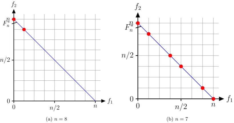
Definition 2.2(OneMinMax_{). A pseudo-Boolean function{0,1}}n_→N2 _{with the objective}

func-tions

OneMinMax_{(x1, . . . , xn) :=}

n

X

i=1

xi, n− n

X

i=1

xi

!

,

where the aim is to maximise the number of ones and zeroes at the same time (see Figure1a).

Definition 2.3(Leading Ones, Trailing Zeroes,LOTZ_{). A pseudo-Boolean function{0,1}}n _→N2

defined as

LOTZ_{(x1, . . . , xn) :=}





n

X

i=1 i

Y

j=1

xj, n

X

i=1 n

Y

j=i

(1−xj)



,

where the goal is to simultaneously maximise the number of leading ones and trailing zeroes (see Figure1b).

OneMinMax_{has the property that every single solution represents a point in the Pareto front}

and that no search point is strictly dominated by another one. The goal is to cover the whole Pareto front, i. e., to compute a set of individuals that contains for eachi, 0≤i≤n, an individual with exactly i ones. In the case of LOTZ_{, all non-Pareto optimal decision vectors only have}

OMM₂

OMM₁

F∗

n

11111111 00000000

00101011

0 n/2 n

0 _n/2 n

(a)OneMinMax.

LOTZ₂

LOTZ₁

0 n/2 n

0 _n/2 n

F1 Fn−2 Fn−1 F∗

n

0******1 11110**1

11111111 00000000

11110000

(b)LOTZ.

Figure 1: Sketches of the functionsOneMinMax₍OMM_{) and}LOTZ_{withn= 8.}

the analysis of the population-based algorithms, which certainly cannot be expected from other multi-objective optimisation problems. Note that the Pareto front forLOTZ_{is given by the set}

ofn+ 1 search points{1i₀n−i_|0≤i≤n}.

We focus our analysis on two simple MOEAs, SEMO and its variant called Global SEMO (GSEMO) because of their simplicity and suitability for a rigorous theoretical analysis. SEMO starts with an initial solutions∈ {0,1}n_{chosen uniformly at random. All non-dominated solutions} are stored in the populationP. Then, it selects a solution suniformly at random fromP, and a new search points′ _{is produced by the mutation step which flips one bit ofschosen uniformly at} random. The new population contains for each non-dominated fitness vectorf(s), s∈P∪ {s′_}, one corresponding search point (dominated individuals are removed from the population), and in the case wheref(s′_{) is not dominated, s}′ _{is added toP (see Algorithm1).}

Algorithm 1SEMO

1: Choose an initial solutions∈ {0,1}n uniformly at random. 2: Determinef(s) and initializeP :={s}.

3: whilestopping criterionnotmetdo

4: Choosesuniformly at random fromP.

5: Choosei∈ {1, . . . , n} uniformly at random.

6: Defines′ _{by flipping the i-th bit ofs.}

7: if s′ _{isnotdominated by any individual inP then}

8: Adds′ toP, and remove all individuals weakly dominated bys′ fromP.

9: end if

10: end while

For SEMO, we know that the expected running time onOneMinMax_{is at mostO(n}2_logn)

[11]. We prove that this upper bound is asymptotically tight.

Theorem 2.4. The expected time for SEMO to cover the whole Pareto front on OneMinMax_is

Θ(n2_logn).

Proof. The upper bound was shown in [11]. For the lower bound, let |x|₁ denote the number of 1-bits and |x|₀ denote the number of 0-bits in x. Define Xt := minx∈Pt{|x|1} if for the initial search pointx0we have|x0|1≥n/2, andXt:= minx∈Pt{|x|0}otherwise. Note that, by definition, X0≥n/2. Now,Xt= 0 is a necessary requirement for covering the whole Pareto front at time t. Hence we lower-bound the sought time by the expected time forXtto reach value 0.

Since only local mutations are used, Xt can only decrease by 1. In order to decrease Xt we have to select a parent with Hamming distanceXt to 0n or 1n, respectively, which happens with probability 1/|Pt|. Note that |Pt| ≥ n/2−Xt as the population contains individuals with

1n_{, respectively. Hence}

Prob(Xt+1=Xt−1|Xt)≤ 1

n/2−Xt ·Xt

n .

The total expected time to decreaseXtto 0 is thus at least

n/2

X

j=1

n

2 −j

n

j =

n/2

X

j=1

n2 2j −

n/2

X

j=1

n=n 2_lnn

2 −O(n 2₎

asPn/2

j=11/j≥lnn/2 = lnn−ln 2.

The reason for the relatively high running time is that the growing population slows down exploration. The population can only expand on the Pareto front in case search points with the current highest or lowest number of ones are chosen (corresponding to a minimumXt-value in the proof of Theorem2.4). Once the population has grown to a size ofµ= Θ(n), the probability that this happens has decreased to Θ(1/n). This means that only a ∼1/n-th fraction of the time the algorithm has a chance to expand on the Pareto front! Uniform parent selection means that most steps are spent idling. The same effect occurs for SEMO onLOTZ_{as proved in [13].}

Theorem 2.5 (Lemma 2 in [13]). The expected time for SEMO to cover the whole Pareto front

on LOTZ_isΘ(n3_).

In the case of GSEMO, a new solution s′ _{is created by flipping each bit from a solution s} independently with probability 1/n, then it proceeds in the same way as SEMO (see Algorithm

2). For GSEMO we have upper bounds of the same order, O(n2_{logn) forOneMinMax[11] and}

O(n3_{) forLOTZ[10], though no lower matching bound is available in the literature for the case} of GSEMO onLOTZ_.

Algorithm 2GSEMO

1: Choose an initial solutions∈ {0,1}n uniformly at random. 2: Determinef(s) and initializeP :={s}.

3: whilestopping criterionnotmetdo

4: Choosesuniformly at random fromP.

5: Defines′ _{by flipping each bit insindependently with probability 1/n.} 6: if s′ _{isnotdominated by any individual inP then}

7: Adds′ _{toP, and remove all individuals weakly dominated bys}′ _fromP.

8: end if

9: end while

We remark that LOTZ _{can also be optimised more efficiently, in time O(n}2_{), by a tailored}

algorithm that uses local search along individual objectives during initialisation to locate both extreme points of the Pareto front, 0n _{and 1}n_{, and then uses crossover to produce the whole} Pareto front from these points [17]. Incorporating a fairness mechanism which makes sure that each individual produces roughly the same number of offspring into SEMO leads to the algorithm FEMO. For FEMO a runtime bound of Θ(n2_{logn) has been given in [13]. The runtime analysis} provided forIBEA_{in [15] gives an upper bound of O(n}2_{logn) and O(n}3_{) for}OneMinMax_and LOTZ_{, respectively, if the population size is set ton+ 1 and therefore does not improve on the}

results for SEMO given in [13].

Our aim is to develop rigorous runtime bounds of SEMO and GSEMO introducing different diversity-based parent selection. We want to study how these mechanisms help to improve the performance of the MOEAs.

3

Diversity-Based Parent Selection

selection of a reference point. In particular, given a reference point r ∈ Rm_{, the hypervolume} indicator is defined on a setP ⊂S as

IH(P) =λ [

x∈P

[f1(x), r1]×[f2(x), r2]× · · · ×[fm(x), rm]

!

whereλ(S) denotes the Lebesgue measure of a setSand [f1(a), r1]×[f2(a), r2]× · · · ×[fm(a), rm] is the orthotope with f(a) and r in opposite corners. We define the contribution of an element

x∈P to the hypervolume of a set of elementsP as

HVC_{(x, P) = IH(P)−IH(P\ {x}).}

The calculation of hypervolume indicator and the calculation of the contribution are both NP-hard when the number of objectivesmis a parameter [3, 4]. However, both can be computed in polynomial time ifm is fixed. In the following, for bi-objective problems like OneMinMax_and LOTZ_{, we can directly calculate the contribution of an element by taking into account the two}

direct neighbours in the objective space as follows.

Definition 3.1 (Hypervolume contribution). For a given reference point r = (r1, r2), we set

f1(x0) =r1andf2(xµ+1) =r2wherex0andxµ+1are individuals used to estimate the hypervolume contribution, and hereinafter µ denotes the size of the current population in SEMO/GSEMO. Furthermore, we assume thatr1=f1(x0)< f1(x1),r2=f2(xµ+1)< f2(xµ).

Let the population be sorted according to the value off1(xi)such that

f1(x0)< f1(x1)< f1(x2)<· · ·< f1(xµ).

The contribution of an individualxi to the hypervolume of a populationP is then given by

HVC_{(xi, P) = (f1(xi)−f1(xi−1))·(f2(xi)−f2(xi+1)).}

Another diversity metric applied to our framework is the crowding distance used in NSGA-II_{[7]. The crowding distance operator measures the density of solutions surrounding a particular}

solution in the population. A solution with a lower crowding distance value implies that the region occupied by this solution is crowded by other solutions. The solutions with a higher crowding distance value are chosen/preferred for reproduction.

Since both SEMO and GSEMO use a population of non-dominated individuals, i. e., all individ-ual have the minimum non-domination rank possible, we can directly apply the crowding distance as our diversity metric (Algorithm3). The population is sorted for each objective function value in increasing order of magnitude. Thereafter, for each objective function, the boundary solutions (solutions with smallest and largest function values) are assigned an infinite distance value. All other intermediate solutions are assigned a distance value equal to the absolute normalised differ-ence of the function values of two adjacent solutions (see Line9of Algorithm3,fmax

m andfmminare the maximum and minimum values of them-th objective function).

Algorithm 3Crowding Distance Operator

1: Letl:=|P|.

2: for alli individuals∈P do

3: SetP[i].distance:= 0

4: end for

5: for allm objectivesdo

6: SortP according tomobjective function value in ascending order.

7: P[1].distance:=P[l].distance:=∞. 8: for i= 2to l−1 do

9: P[i].distance:=P[i].distance+P[i+1].m−P[i−1].m

fmax

m −f

min

m

10: end for

11: end for

GSEMO the number of function evaluations coincides with the number of generations needed as each generation only creates one new offspring whose fitness is evaluated.

For the hypervolume contribution (HVC), according to Definition3.1, the reference point can be defined so that the current extreme individuals in the population and individuals in intermediate empty areas have a high diversity score, and a strong influence for the algorithm. In the case of the crowding distance contribution (CDC) the same behaviour applies, extreme points in the search space receive a high distance while intermediate individuals surrounded by empty areas receive a higher distance than the ones where the area is more crowded.

With this information we can define selection mechanisms capable of selecting those extreme points and pushing the spread of the population toward the outer areas of the search space. However, as our theoretical analysis will show, in case the population already contains the extreme points of the Pareto front (0nand 1nforOneMinMax_andLOTZ_{), we need to be flexible enough}

to ignore those points and select intermediate individuals surrounded by empty areas in the search space to fully cover the Pareto front.

The selection mechanisms defined in this paper use the previous diversity contribution metrics but any other metric can be easily applied that follows the behaviour mentioned before. Firstly, we define 3 different rank-based selection schemes in which the probability of selecting individuals with a high diversity score is higher than for individuals with a lower diversity score (see Definition3.2). The first is calledexponential; it is a rather aggressive scheme that strongly favours the best-ranked individuals and has a very small tail. The second is calledpower law as it follows a power law distribution; it is much less aggressive with a fat tail and yet a constant probability of selecting the first constant ranks. And finally, the third ranking scheme is calledharmonic; it is the least aggressive scheme with a fat tail and only a probability ofO(1/(logµ)) for selecting the best few individuals.

Definition 3.2 (Rank-based selection schemes). The probability of selecting thei-th ranked

indi-vidual is

2−i µ

X

j=1 2−j

, 1/i

2

µ

X

j=1 1

j2

, µ1/i

X

j=1 1

j

for the exponential, power law, and harmonic ranking scheme (see Figure2), respectively.

2 4 6 8 10

0 0.2 0.4 0.6

Rank of diversity metric

S

el

ec

ti

on

p

rob

ab

il

it

y Exponential: ∼2−i

Power law: ∼1/i2

Harmonic: ∼1/i

Figure 2: Rank-based selection schemes and their selection probabilities.

Secondly, we use the classical tournament selection, but with a specific tournament size ofµ, the current size of the population. This means we choose µ individuals uniformly at random with replacement from the population and then select the individual with the highest diversity contribution from this multi-set. Selection with replacement implies that there is a chance of not selecting particular individuals, while other individuals might be picked multiple times.

the diversity-based parent selection method. Then we continue as in the original algorithms. Our parent selection mechanisms are not limited to these algorithms and may prove useful on a much broader class of MOEAs.

Algorithm 4SEMO with diversity-based parent selection

1: Choose an initial solutions∈ {0,1}n uniformly at random. 2: Determinef(s) and initializeP :={s}.

3: whilestopping criterionnotmetdo

4: Estimate diversity contribution∀s∈P.

5: Chooses∈P according to the parent selection mechanism.

6: Choosei∈ {1, . . . , n} uniformly at random.

7: Defines′ _{by flipping the i-th bit ofs.}

8: if s′ _{isnotdominated by any individual inP then}

9: Adds′ toP, and remove all individuals weakly dominated bys′ fromP.

10: end if

11: end while

Algorithm 5GSEMO with diversity-based parent selection

1: Choose an initial solutions∈ {0,1}n _{uniformly at random.}

2: Determinef(s) and initializeP :={s}.

3: whilestopping criterionnotmetdo

4: Estimate diversity contribution∀s∈P.

5: Chooses∈P according to the parent selection mechanism.

6: Creates′ by flipping each bit insindependently with probability 1/n. 7: if s′ isnotdominated by any individual inP then

8: Adds′ toP, and remove all individuals weakly dominated bys′ fromP.

9: end if

10: end while

4

On Diversity-Based Progress

We show that diversity-based parent selection mechanisms can achieve a fast spread on the Pareto front. The following arguments and analyses consider the situation where the population is located on the Pareto front. This is trivially the case forOneMinMax _{as all search points are}

Pareto-optimal. For LOTZ_{we later supply a separate analysis that covers the process of reaching the}

Pareto front.

For OneMinMax _and LOTZ _{the most promising parents are those that have a Hamming}

neighbour that is on the Pareto set, but not yet contained in the population. We call these search pointsgood:

Definition 4.1(good individuals). With reference to a populationP and a fitness function with

Pareto frontF∗ _{and corresponding Pareto setX}∗_{, we call a search pointx∈P∩X}∗ _{goodif there} is a Hamming neighboury of xsuch thaty ∈X∗ _{but f(y)6∈f(P) wheref(P)denotes the set of} objective vectors of populationP. Otherwise,xis called bad.

A diversity measure should encourage the selection of such good individuals.

Definition 4.2 (diversity-favouring). We call a measure C_{(x, P) diversity-favouring on S ⊆}

{0,1}n _{with respect to a fitness function with Pareto front F}∗ _{if for all populations P and all} x, y∈P∩X∗∩S we have the following: ifxis bad and y is good thenC_{(x, P)<}C_{(y, P).}

Lemma 4.3. The hypervolume contributionHVC_{(x, P)is diversity-favouring on{0,1}}n_\{0n_,1n_}

for both OneMinMax_and LOTZ_{if the reference point is dominated by (−1,−1).}

Proof. Let us consider an individual xi∈ {/ 0n,1n}of the sorted population according tof1, using the notation from Definition3.1. Ifxi is bad, then there are Hamming neighboursxi−1and xi+1 of xi in P, the HVC(xi, P) is the minimum possible, sincef1(xi)−f1(xi−1) = 1 and f2(xi)− f2(xi+1) = 1 yieldingHVC_{(xi, P) = (f1(xi)−f1(xi−1))·(f2(xi)−f2(xi+1)) = 1.}

Now, let us consider a good search pointyi, that is,yi−1 oryi+1 is not a Hamming neighbour ofyi. Then we havef1(yi)−f1(yi−1)>1 orf2(yi)−f2(yi+1)>1 and in any caseHVC(yi, P) = (f1(yi)−f1(yi−1))·(f2(yi)−f2(yi+1))>1. ThusHVC(yi, P)>HVC(xi, P), which completes the proof.

Lemma 4.4. The crowding distance contribution CDC_{(x, P) is diversity-favouring on {0,1}}n_\

{0n_,1n_{} for both OneMinMaxand LOTZ.}

Proof. By Algorithm 3 the search points with the minimum and maximum f1 score in the pop-ulation are going to have infinite diversity score, regardless of the objective chosen to sort the population.

Let us say that there is a bad individualxi with Hamming neighboursxi−1andxi+1 contained in P. According to the numerator of Line 9 of Algorithm3, the difference between the f1(xi−1) (or f2(xi−1)) and f1(xi+1) is the minimum possible, which means the minimum CDC(xi, P) is assigned to the individualxi.

In the case of a good search pointyi, that is,yi−1 or yi+1 are not Hamming neighbours of yi, the difference between the next contained search points in P is higher. If the difference between

f1(yi) (or f2(yi)) is higher than the minimum possible, this means CDC_{(xi, P) <} CDC_{(yi, P)}

which completes the proof.

Note that in both above measures 0n_{and 1}n_{, if contained in the population, will always receive} a high score, regardless of whether they are good or bad. If they are bad, there is a high chance that a bad individual will be selected as parent in a diversity-based parent selection mechanism. With this in mind, the probability of selecting a good individual can be bounded from below as follows.

Lemma 4.5. Let C_{(x, P)be a diversity-favouring measure on{0,1}}n_{\ {0}n_,1n_{}. Consider either}

OneMinMax _or LOTZ _{and assume the population P is a subset of the Pareto set, P ⊆ X}∗_.

Imagine P being sorted according to non-increasing C_{(x, P) values. Consider a parent selection}

mechanism based on C_{(x, P) such that ri is the probability of selecting the i-th element of P in}

the sorted sequence. Then the probability of selecting a good individual is at least min{r1, r2, r3} unlessP already covers the Pareto front.

Proof. Before the whole Pareto front is covered by the populationP, there exists at least one good individualxin populationP with no corresponding Hamming neighbour sin the Pareto set X∗_. Then the individuals which correspond to the Hamming neighbours of the missing pointsare good search points.

SinceC_{(x, P) is defined as a diversity-favouring measure on{0,1}}n_{\ {0}n_,1n_{}, the good search}

points have higher contribution than bad search points that are neither 0n_{nor 1}n_{. Therefore, among} the top three ranked elements inP, there exists at least one good individual. The probability of selecting this good individual is at least min{r1, r2, r3}.

The parent selection mechanisms thus have the following probability of selecting good individ-uals.

Lemma 4.6. In the setting described in Lemma 4.5, the probability pgood of selecting a good

individual is

1. Ω(1)for the exponential and power law ranking schemes,

2. Ω(1/logµ)for the harmonic ranking scheme,

Proof. For the parent selection with the exponential ranking scheme, the probability follows from Lemma4.5, which fulfils

r1≥r2≥r3= 2−3 µ

X

j=1 2−j

≥2−3= Ω(1).

For the power law ranking scheme, sincePµ

j=1j12 ≤

P∞

j=1 j12 =π

2_{/6, the probability fulfils}

r1≥r2≥r3= 1/32 µ X j=1 1 j2 ≥ 2

3·π2 = Ω(1).

In the case of the harmonic ranking scheme, sincePµ

j=1 1

j ≤lnµ+ 1, the probability fulfils

r1≥r2≥r3= 1µ/3

X

j=1 1

j

≥ 1

3·(lnµ+ 1) = Ω(1/logµ).

For tournament selection, the probability of selecting a good individual is at least min{r1, r2, r3} andr1≥r2≥r3. In order for the individual with the 3rd maximum contribution to be selected in the tournament selection, the individuals with the 1st and 2nd maximum contribution should never be selected in theµtimes (probability of (1−2/µ)µ). And, conditional on this happening, the individual with the 3rd maximum contribution has to be chosen at least once amongst the otherµ−2 individuals in the µtimes with probability 1−1− 1

µ−2

µ

. Hence, the probability of selecting a good individual is at least

pgood≥

1−

1− 1 µ−2

µ

·

1− 2 µ

µ

≥

1−1 e

·

1−2 µ

µ

using 1−1_xx

≤1/e forx >1. Sincef(x) = 1−1_xx

is non-decreasing when x≥1, withµ≥3,

1−_µ2

µ

2

≥ 1−2₃32

≥0.19. Therefore,pgood≥ 1−1_e·0.192= Ω(1).

5

Speedups on OneMinMax

For any parent selection mechanism defined before, the parent selection is focused on selecting an individual with a high diversity score. In the case of HVC or CDC, having a high diversity contribution means that, apart from the possible exceptions of 0n _{and 1}n_{, the parent will be} good, i. e., located in a less populated area of the Pareto front. We show that by preferring good individuals in the parent selection, SEMO and GSEMO can quickly find the whole Pareto front forOneMinMax_.

Lemma 5.1. Suppose that the probability of selecting a good individual is at leastpgood. Then the

expected runtime for SEMO or GSEMO to find all solutions in the Pareto front on OneMinMax

is bounded above byO((nlogn)/pgood).

Proof. We call a step arelevant stepif the algorithm selects a good parent on the Pareto front. We show in the following thatO(nlogn) relevant steps are sufficient for covering the whole Pareto front of OneMinMax_{, regardless of irrelevant steps performed. This shows the claim as the expected}

time for a relevant step is 1/pgood.

We use theaccounting method (see, e. g., Section 17.2 in [5]) to bound the number of relevant steps. Specifically, we count the number of relevant steps spent in selecting a good parent withi

ones. Summing up (upper bounds on) all these times across all 0≤i≤nwill imply the claim. Note that, once potential gaps ati−1 andi+ 1 are filled, there can be no more relevant steps ationes, due to the definition of a relevant step. Hence the expected number of relevant steps at

creating an individual withi+ 1 ones is at least (n−i)/n·(1−1/n)n−1_{≥(n−i)/(en) (this holds} both for SEMO and GSEMO; for SEMO the factor 1/ecan be removed). The time for filling both gaps is at mosten/i+en/(n−i). Hence there are at mosten/i+en/(n−i) relevant steps selecting a parent withiones. In the special cases of i= 0 or i=nthe time to fill the neighbouring gaps simplifies toen/n=e.

Summing over alli, the expected total number of relevant steps is hence at most

2e+ n−1

X

i=1

en i +

en n−i

= 2e+ 2 n−1

X

i=1

en i = 2

n

X

i=1

en

i ≤2en(logn+ 1).

Where the summation Hn = Pn

i=11/i is known as the harmonic number and satisfies Hn = lnn+ Θ(1) this completes the proof.

Combining Lemma 4.6 and Lemma 5.1, we have proved the following results. Note that the population sizeµ is always at most n+ 1 on OneMinMax_and LOTZ_{, hence for the harmonic}

ranking scheme,pgood= Ω(1/logµ) = Ω(1/logn).

Theorem 5.2. Consider SEMO and GSEMO with diversity-based parent selection using any

di-versity measure that is didi-versity-favouring on {0,1}n _{\ {0}n_,1n_{} (e. g. HVC or CDC). Then the} expected time to find the whole Pareto front on OneMinMax _{is bounded by O(nlogn) for the}

exponential and power law ranking schemes, and for tournament selection with tournament sizeµ. It is bounded byO(nlog2n)for the harmonic ranking scheme.

As both SEMO and GSEMO with the classical uniform parent selection need time Θ(n2_logn) onOneMinMax_{, our parent selection schemes lead to speedups of order Θ(n) and Θ(n/logn),}

respectively.

6

Speedups on LOTZ

We now turn to the functionLOTZ_{. In contrast to}OneMinMax_{, where all individuals are Pareto}

optimal, for LOTZ _{we have to estimate the time for the population to reach the Pareto front.}

For SEMO the approach to the Pareto front can be estimated easily since SEMO keeps only one individual in the population. For local mutations as used in SEMO, whenever an offspring is created, either the offspring dominates the parent, or the parent dominates the offspring (or both, if they have the same function values). The population size remains unchanged before there is a solution on the Pareto front. For any parent on the Pareto front, SEMO only accepts its offspring if it is also on the Pareto front, otherwise the offspring is dominated by the parent.

Lemma 6.1. The expected time for SEMO to reach the Pareto front is O(n2_{). Assume that}

afterwards the probability of selecting a good individual in the population is at least pgood. The expected runtime for SEMO to reach a population covering the whole Pareto front on LOTZ _is

bounded above byO(n2_/pgood).

Proof. The time for the population to find the first Pareto-optimal point isO(n2_{) and has already} been proved in Lemma 1 in [13]. So we can focus on the time required to find the whole Pareto front. By theaccounting method used to prove Lemma5.1and the definition of relevant step: the algorithm selects a good parent on the Pareto front, we count the number of relevant steps spent selecting a good parent withileading ones, 1i₀n−i_{, and sum up all these times across all 0≤i≤n} to prove the claim.

The potential gaps consist of non-existing non-dominated individuals ati−1 andi+1 (1i−1₀n−i+1 and 1i+10n−i−1, respectively). It is necessary to fill those gaps by including these search points in the population. Once this has happened, there can be no more relevant steps at i leading ones. So the expected number of mutations at i leading ones is bounded by the expected number of mutations fromi needed to filli−1 andi+ 1. If 1i₀n−i _{is selected as parent, the probability of} mutation creating 1i−1₀n−i+1_{or 1}i+1₀n−i−1_{is 1/n, respectively. The time for filling both gaps (if} existent) is at mostn+n. Hence there are in expectation at most 2n relevant steps selecting a parent withileading ones.

Summing over alli, the expected total number of relevant steps is hence at most

n

X

i=0

Algorithm 6Modified Global SEMO with diversity-based parent selection

1: Choose an initial solutions∈ {0,1}n _{uniformly at random.}

2: Determinef(s) and initializeP :={s}.

3: whilestopping criterionnotmetdo

4: LetP′ ⊆P be the set of all search points with a maximum L-dominant attribute in P. 5: Estimate diversity contribution∀s∈P′ w. r. t. the populationP′.

6: Chooses∈P′ according to parent selection mechanism.

7: Creates′ by flipping each bit ofsindependently with probability 1/n. 8: if s′ isnotdominated by any individual inP then

9: Adds′ toP, and remove all individuals weakly dominated bys′ fromP.

10: end if

11: end while

Noting that the expected waiting time for a relevant step is 1/pgood. Thus the overall expected runtime for SEMO to achieve a population covering the whole Pareto front on LOTZ_{is upper}

bounded byO(n2_{) +O(n}2_{/pgood) =O(n}2_/pgood).

Combining Lemma4.6and Lemma 6.1, we now have proved the following results.

Theorem 6.2. Consider SEMO with diversity-based parent selection using any diversity measure

that is diversity-favouring on{0,1}n_{\ {0}n_,1n_{}(e. g. HVC or CDC). Then the expected time to find} the whole Pareto front on LOTZ_{is bounded byO(n}2_{)for the exponential and power law ranking}

schemes, and for tournament selection with tournament size µ. It is bounded byO(n2_{logn) for} the harmonic ranking scheme.

The analysis of GSEMO turns out to be more difficult than the analysis of SEMO. The reason is that the approach to the Pareto front becomes harder to analyse. With global mutations, GSEMO can create incomparable search points while approaching the Pareto front. This means that the population can expand in size while approaching the Pareto front, and even after the whole population has reached the Pareto front, it is possible to create search points off the Pareto front that are accepted in the population.

Experiments in Section 7 indicate that this behaviour does not slow down the algorithm by more than a constant factor. However, proving that the boundO(n2_{) for SEMO also holds for} GSEMO turns out to be very challenging. We therefore take a different approach and analyse a modified variant of GSEMO that is easier to analyse. Experiments presented in Section7confirm that this modification does not significantly change the average runtime (inspecting Tables3and4, the quotients of average times for the modified GSEMO and those for the original GSEMO across all parent selection mechanisms are 0.88 for HVC_{(−1,−1), 1.19 for} HVC_{(−n,−n), and 1.27 for}

CDC, averaging to 1.1 are close to 1 in many settings and always in the interval [0.48,2.03]). The idea behind this modification is to simplify the approach to the Pareto front by restricting parent selection to search points that are maximal with regards to a linear combination of both objectives.

Definition 6.3 (L-dominant attribute). Let L(x) = LO(x) + TZ(x), where LO(x) and TZ(x)

denotes the total number of leading ones and the total number of trailing zeros of a certain individual

x, respectively.

We modify GSEMO in such a way that it only picks parents with maximal L-dominant attribute in the population (see Algorithm 6), and also the computation of the diversity contribution is restricted to these search points. This has two effects: it simplifies and facilitates the analysis of the individuals while they are approaching the Pareto front. While the original GSEMO can store incomparable search points with different L-values in the population, the modified GSEMO only considers incomparable search points with maximum L-value. In addition, since allxindividuals on the Pareto front have the largest possible value of L(x) =n, once the Pareto front is reached, the algorithm only selects individuals on the Pareto front as parents according to their diversity contribution.

We first bound the expected time to reach the Pareto front.

Lemma 6.4. The expected time for the modified GSEMO to reach the Pareto front is bounded

Proof. According to Definition6.3, before reaching the Pareto front, the solution with maxx∈P(L(x)) is selected to generate an offspring. Consider the event of only flipping the first 0-bit or the last 1-bit of the selected individual. Since the offspring from this event has a higher value of one of the objectives than its parent which is of the maximum L(x) in the population, the offspring is non-dominated by any individuals in the population and is accepted by the algorithm. Hence, the probability of increasing maxx∈P(L(x)) is at least

2· 1 n·

1− 1 n

n−1

≥ 2 en.

Throughout the process, the value of maxx∈P(L(x)) in the population never goes down. There-fore, the overall expected runtime for GSEMO with this selection scheme to reach the Pareto front is at most

n−2

X

Lmax=0

en

2 =O(n 2_).

Lemma 6.5. Assume that the probability of selecting a good individual in the population is at least

pgood. The expected time for the modified GSEMO to reach a population covering the whole Pareto front on LOTZ_{is bounded above byO(n}2_/pgood).

Proof. As for SEMO, before the population covers the whole Pareto front, the optimisation process of the modified GSEMO can be divided into two stages. The first stage focusses on obtaining the first individual on the Pareto front and the second one focusses on covering the Pareto front. As proved in Lemma6.4, the expected time for the modified GSEMO to reach the Pareto front is at mostO(n2_).

In the second stage, by following the definition of relevant step, the parent to be selected is a good search point on the Pareto front with the maximum L(x) dominant attribute. The algorithm will select individuals on the Pareto front with the maximum L(x) dominant attribute according to their diversity contribution. So now we can apply the accounting method used to prove previous lemmas to bound the number of relevant steps spent selecting the good parent.

As in Lemma 6.1, we define a good parent with i leading ones with possible gaps on i−1 and/ori+ 1 across all 0≤i≤n. And by introducing the factor 1/eto the analysis in Lemma6.1, we now have the time for filling both gaps is at most 1/(en) + 1/(en). Hence there are at most

en+en= 2enrelevant steps selecting a good parent withileading ones. Summing over alli, the expected total number of relevant steps is hence at most

n

X

i=0

2en= 2e

n

X

i=0

n=O(n2₎

The overall runtime for the modified GSEMO onLOTZ_{to reach a population covering the whole}

Pareto front is bounded above byO(n2_/pgood).

As mentioned on the proof of the previous lemma, once the individual with the maximum L(x) dominant attribute has reached the Pareto front, the algorithm will always select good individuals on the Pareto front (with the maximum L(x) dominant attribute) according to their diversity contribution. This characteristic allows us to apply Lemma4.6, and by Lemma6.5, we now have proved the following results.

Theorem 6.6. Consider the modified GSEMO with diversity-based parent selection using any

diversity measure that is diversity-favouring on {0,1}n_{\ {0}n_,1n_{} (e. g. HVC or CDC). Then the} expected time to find the whole Pareto front on LOTZ_{is bounded byO(n}2_{)for the exponential and} power law ranking schemes, and for tournament selection with tournament size µ. It is bounded byO(n2_{logn)for the harmonic ranking scheme.}

7

Experiments

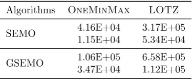
Table 1: Mean (first rows) and STD (second rows) of generations required to find the Pareto front for SEMO and GSEMO onOneMinMax_andLOTZ_{withn= 100.}

Algorithms OneMinMax LOTZ

SEMO 4.16E+04 3.17E+05 1.15E+04 5.34E+04

GSEMO 1.06E+05 6.58E+05 3.47E+04 1.12E+05

the case of the modified GSEMO, we measure its performance only on LOTZ_{and we compare}

its performance to GSEMO in order to observe the impact of the L-dominant attribute on the performance of the algorithm.

Experiments also allow for a more detailed comparison of the HVC, CDC, and the parent selection methods. In the case of the HVC, we have defined two settings for the reference points, (−1,−1) and (−n,−n). For the first reference point, a slight preference to the extreme points is provided while with the second, the influence of the extreme points becomes very strong. This particular characteristic became an interesting feature to observe in the case of the ranking-based selection schemes, and exposes a potential flaw for the case of HVC with low (or high in the case of minimisation) reference point or CDC (since it assigns infinite value to the extreme points) and the parent selection mechanisms that focus very aggressively toward the extreme points, as we shall see below.

Since we are interested in the time required to find the Pareto front, we report the following outcomes and stopping criteria for each run. Success, the whole Pareto front has been covered, i. e., the run is stopped if the population contains all individuals on the Pareto front. Failure/Stagnation, once the run has reached 1 million generations and the Pareto front has not been fully covered, this is enough time for the algorithms to create new individuals and fill the gaps on the Pareto front. We repeat the experimental framework for 100 runs with problem sizen= 100 for all algorithmic approaches and report the mean and standard deviation (STD) as our metrics of interest.

Table1shows the mean and STD of generations required to find the Pareto front for the classic SEMO and GSEMO that use uniform parent selection for both test functions. Table2and3refer to the mean and standard deviation of generations required to find the Pareto front for SEMO and GSEMO with the different diversity-based parent selection schemes forOneMinMax_andLOTZ_,

respectively. Finally, Table4 shows the mean and standard deviation of generations required to find the Pareto front for the modified GSEMO onLOTZ_.

As we mentioned before, a parent selection mechanisms that is extremely focused on the extreme points can be potentially dangerous, and to exemplify this, we have introduced a deterministic selection mechanism which we have namedHighest Diversity Contribution (HDC): always select an individual with the highest diversity contribution (break ties uniformly at random if there are several such points). We also have defined a modified version of the uniform random selection used by SEMO and GSEMO, that we callNon-Minimum Uniform at Random (NMUAR), where the individuals with the minimum diversity contribution in the population are ignored (provided that the population does contain multiple diversity contribution values) and one individual is selected uniformly at random from all remaining individuals. In this sense individuals with high diversity contributions have better probabilities to be selected and the approach is flexible enough to choose between extreme and intermediate individuals.

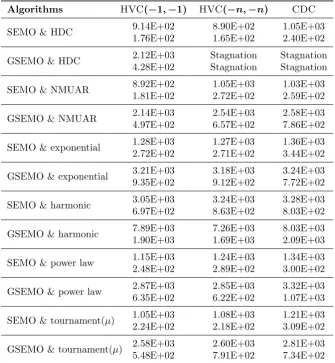
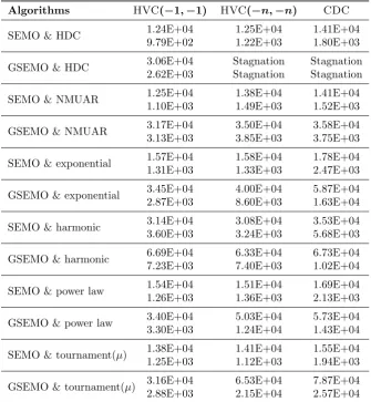
As it can be observed in Table 2 and3, HDC fails to find the Pareto front forOneMinMax

andLOTZ_{in the case of GSEMO for both diversity-based metrics. For the case of GSEMO with}

HDC selection mechanism with HVC and CDC on OneMinMax _{the failure rate was 0.94 and}

0.93, respectively. OnLOTZ_{, the failure rate was 1.0 for both diversity metrics.}

The reason for these bad results for GSEMO (and the modified GSEMO) on OneMinMax_is

due to the mutation operator. Both algorithms can create gaps by creating an offspring that may differ from its parent with more than one bit. In the case of GSEMO onLOTZ_{, the algorithm}

Table 2: Mean (first rows) and STD (second rows) of generations required to find the Pareto front for SEMO and GSEMO with diversity-based parent selection methods on OneMinMax

withn= 100. “Stagnation” indicates a failure rate larger than 0.

Algorithms HVC₍₋₁,−1) HVC(−n,−n) CDC

SEMO & HDC 9.14E+02 8.90E+02 1.05E+03 1.76E+02 1.65E+02 2.40E+02

GSEMO & HDC 2.12E+03 Stagnation Stagnation 4.28E+02 Stagnation Stagnation

SEMO & NMUAR 8.92E+02 1.05E+03 1.03E+03 1.81E+02 2.72E+02 2.59E+02

GSEMO & NMUAR 2₄._.14E+03_{97E+02 6}2._.54E+03_{57E+02 7}2_..58E+03_86E+02

SEMO & exponential 1.28E+03 1.27E+03 1.36E+03 2.72E+02 2.71E+02 3.44E+02

GSEMO & exponential 3.21E+03 3.18E+03 3.24E+03 9.35E+02 9.12E+02 7.72E+02

SEMO & harmonic 3.05E+03 3.24E+03 3.28E+03 6.97E+02 8.63E+02 8.03E+02

GSEMO & harmonic 7.89E+03 7.26E+03 8.03E+03 1.90E+03 1.69E+03 2.09E+03

SEMO & power law 1.15E+03 1.24E+03 1.34E+03 2.48E+02 2.89E+02 3.00E+02

GSEMO & power law 2.87E+03 2.85E+03 3.32E+03 6.35E+02 6.22E+02 1.07E+03

SEMO & tournament(µ) 1.05E+03 1.08E+03 1.21E+03 2.24E+02 2.18E+02 3.09E+02

Table 3: Mean (first rows) and STD (second rows) of generations required to find the Pareto front for SEMO and GSEMO with diversity-based parent selection methods onLOTZ_{with n = 100.}

“Stagnation” indicates a failure rate larger than 0.

Algorithms HVC₍₋₁,−1) HVC(−n,−n) CDC

SEMO & HDC 1.24E+04 1.25E+04 1.41E+04 9.79E+02 1.22E+03 1.80E+03

GSEMO & HDC 3.06E+04 Stagnation Stagnation 2.62E+03 Stagnation Stagnation

SEMO & NMUAR 1.25E+04 1.38E+04 1.41E+04 1.10E+03 1.49E+03 1.52E+03

GSEMO & NMUAR 3₃._.17E+04_{13E+03 3}3._.50E+04_{85E+03 3}3_..58E+04_75E+03

SEMO & exponential 1.57E+04 1.58E+04 1.78E+04 1.31E+03 1.33E+03 2.47E+03

GSEMO & exponential 3.45E+04 4.00E+04 5.87E+04 2.87E+03 8.60E+03 1.63E+04

SEMO & harmonic 3.14E+04 3.08E+04 3.53E+04 3.60E+03 3.24E+03 5.68E+03

GSEMO & harmonic 6.69E+04 6.33E+04 6.73E+04 7.23E+03 7.40E+03 1.02E+04

SEMO & power law 1.54E+04 1.51E+04 1.69E+04 1.26E+03 1.36E+03 2.13E+03

GSEMO & power law 3.40E+04 5.03E+04 5.73E+04 3.30E+03 1.24E+04 1.43E+04

SEMO & tournament(µ) 1.38E+04 1.41E+04 1.55E+04 1.25E+03 1.12E+03 1.94E+03

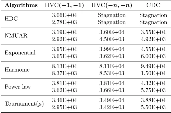
Table 4: Mean (first rows) and STD (second rows) of generations required to find the Pareto front for the modified GSEMO and diversity-based parent selection methods onLOTZ_{with n= 100.}

“Stagnation” indicates a failure rate larger than 0.

Algorithms HVC₍₋₁,−1) HVC(−n,−n) CDC

HDC 3.06E+04 Stagnation Stagnation

2.78E+03 Stagnation Stagnation

NMUAR 3.19E+04 3.60E+04 3.55E+04

2.92E+03 4.50E+03 4.92E+03

Exponential 3.95E+04 3.99E+04 4.55E+04 3.65E+03 3.62E+03 6.00E+03

Harmonic 8₈._.13E+04_{37E+03 8}8._.11E+04_{53E+03 1}9_..49E+04_50E+04

Power law 3.81E+04 3.81E+04 4.32E+04 3.62E+03 3.66E+03 5.75E+03

Tournament(µ) 3.46E+04 3.49E+04 3.88E+04 2.95E+03 3.42E+03 5.50E+03

trailing zero. Then it will continue selecting those individuals ignoring the intermediate ones, leaving the population in astagnation state. This observation also justifies why we introduced parent selection schemes of varying degree of aggressiveness. We analyse this process rigorously in Section8.1.

For all other parent selection schemes defined in this paper, we have achieved a significant speed up in the performance of SEMO and GSEMO of around one order of magnitude. As it can be observed in Table2and3, SEMO and GSEMO with diversity-based parent selection mechanisms are able to find the Pareto front faster than its classical counterparts, i. e., fewer generations are required for both test functions. Note that the problem sizen= 100 is relatively moderate; as our theoretical results prove, speedups over the original algorithms will grow further when the problem size is increased.

In the case of the modified GSEMO, the same stagnation state was reached (see Table4). For the modified GSEMO with HDC selection mechanism with HVC and CDC onOneMinMax_the

failure rate was 0.97 and 1.0, respectively. On LOTZ_{the failure rate for the modified GSEMO}

with HVC and CDC decreases considerably, reaching 0.37 and 0.33, respectively.

The modified GSEMO onLOTZ _{achieved a considerably lower failure rate compared to the}

original GSEMO, where it was 1.0. We believe that there are two reasons for this. Firstly, for the modified GSEMO it is not possible to reach the Pareto front in different areas, avoiding the creation of gaps while approaching the Pareto front; the individual with the largest L-dominant attribute will always reach the Pareto front. Secondly, after the Pareto front has been reached, the algorithm will select individuals on the Pareto front as parents according to their diversity contribution. Here, from the i individual, the mutation operator needs to flip 1i−1₀n−i+1 _{or 1}i+1₀n−i−1 _{to create a} new individual. In this sense it is more difficult to leave an empty space between points leading to this better performance but it is always possible for the algorithm to flip multiple consecutive bits to create a gap, resulting in the mentioned failure rates.

The modified GSEMO can also achieve a significant speed up in performance onLOTZ_{. With}

this preliminary analysis we can see that the introduction of the L-dominant attribute does not drastically change the average runtime and it can be used as an approximation or first step towards the definition of a bound for GSEMO with diversity-based parent selection onLOTZ_.

8

Comparing Selection Schemes: How Much Greed is Good?

where multi-bit flips do a lot of harm by leading the population into a stagnation state.

Finally in Section8.2 we discuss the results obtained regarding the NMUAR mechanism. As shown in Section7, NMUAR performs experimentally well for SEMO and GSEMO with no stag-nation outcome. We show that for a particular choice of the reference point NMUAR can lead the population into a stagnation state. On the positive side, we show that NMUAR is able to efficiently optimise bothLOTZ_andOneMinMax_{for common choices of the reference point.}

8.1

Why Highest Diversity Contribution Stagnates

In this section we theoretically examine the stagnation results of Section7related to GSEMO with the HDC selection strongly favouring the extreme points. As it can be observed from Tables2and

3, a greedy approach seems to be the best for SEMO. SEMO can find all individuals on the Pareto front but also is the fastest in doing so. This is because for SEMO onOneMinMax_{, all individuals}

are part of the Pareto front and the algorithm starts with one individual on the Pareto front. In the case ofLOTZ_{the algorithm always reaches the Pareto front with just one individual. Once on}

the Pareto front, the spread of the population to outer areas can only be achieved by individuals that differ from its parent in just one bit, i. e., no gaps or empty spaces are left between points.

In the following we show by means of rigorous runtime analysis why the previous experimen-tal results occur for the modified GSEMO on LOTZ_{. Let the reference point be dominated by}

(−n2_,−n2_{) for the HVC in order to simplify the analysis for proving that focusing on extreme} points can lead to undesired results. Our main result of this section is the following.

Theorem 8.1. Consider the modified GSEMO with Highest Diversity Contribution, choosing as

diversity metric either CDC or HVC with a reference point dominated by(−n2_,−n2_{)on the} func-tion LOTZ_{. Then at the first point in time the populationPt contains both 0}n _and1n_{,Pt equals}

the whole front with probability Ω(1) and 1−Ω(1). The expected time to find the whole Pareto front isnΩ(n)_.

The remainder of this subsection is devoted to the proof of Theorem8.1. First, we define what a gap means and transition probabilities for mutations on the Pareto front that will be used in the remainder of this section.

Definition 8.2 (Gap). We say that a populationPt has a gap at position i if 1i0n−i ∈/ Pt, but

1j₀n−j_∈P

tand1k0n−k ∈Ptforj < i < k.

Definition 8.3(Transition probabilities). We define

pk =n−k·

1−1 n

n−k

=

1−1 n

n

·(n−1)−k.

as the probability of jumping from any search point1i₀n−i _to1i+k₀n−i−k _and1i−k₀n−i+k _(if exis-tent).

Next, we show that, once the Pareto front has been reached, the Highest Diversity Contribution selection will always choose a parent xwith an extreme number of ones. The following lemma applies to a populationP containing only search points on the Pareto front. This setting applies for the modified GSEMO once the Pareto front has been reached as then parent selection is only based on search points with a maximum L-dominant attribute, corresponding to points on the Pareto front.

Lemma 8.4. Consider the Highest Diversity Contribution (HDC) selection mechanism, choosing

as diversity metric eitherHVC_{(x, P)with reference point dominated by(−n}2_,−n2_{)orCDC(x, P)} on the function LOTZ_{, for a population P containing only search points on the Pareto front.}

Then the parent chosen by HDC will always either have a minimum or a maximum number of ones among all search points inP.

Proof. Let us consider an individualxiof the sorted population according tof1, using the notation from Definition 3.1, and let us definef1(x0)≤ −n2 _{and f2(xµ+1)≤ −n}2 _{as reference point. For} any point xi = 1j0n−j where 1 < i < µ, the highest possible contribution that the point xi can achieve is if it has as neighbours the points x1 = 0n and xµ = 1n, so we have f1(xi) = j,