Determination of an additive time-and space-dependent coefficient in the heat equation

This is a repository copy of Determination of an additive time-and space-dependent coefficient in the heat equation.

White Rose Research Online URL for this paper: http://eprints.whiterose.ac.uk/120994/

Version: Accepted Version

Article:

Huntul, M, Lesnic, D orcid.org/0000-0003-3025-2770 and Johansson, T (2018)

Determination of an additive time-and space-dependent coefficient in the heat equation. International Journal of Numerical Methods for Heat and Fluid Flow, 28 (6). pp. 1352-1373. ISSN 0961-5539

https://doi.org/10.1108/HFF-04-2017-0153

© Emerald Publishing Limited 2018 Published by Emerald Publishing Limited. Licensed re-use rights only. This is an author produced version of a paper published in International Journal of Numerical Methods for Heat & Fluid Flow. Uploaded in accordance with the publisher's self-archiving policy. Available online;

https://doi.org/10.1108/HFF-04-2017-0153.

[email protected] Reuse

Items deposited in White Rose Research Online are protected by copyright, with all rights reserved unless indicated otherwise. They may be downloaded and/or printed for private study, or other acts as permitted by national copyright laws. The publisher or other rights holders may allow further reproduction and re-use of the full text version. This is indicated by the licence information on the White Rose Research Online record for the item.

Takedown

If you consider content in White Rose Research Online to be in breach of UK law, please notify us by

Determination of an additive time- and

space-dependent coefficient in the heat equation

M.J. Huntul1,2_{, D. Lesnic}1 _{and B.T. Johansson}3

1_{Department of Applied Mathematics, University of Leeds, Leeds LS2 9JT, UK}

2_{Department of Mathematics, College of Science, Jazan University, Jazan, Saudia Arabia} 3_{ITN, Campus Norrkoping, Linkoping University, Sweden}

E-mails: [email protected] (M.J. Huntul), [email protected] (D. Lesnic), [email protected] (B.T. Johansson).

Abstract

Purpose - The purpose of this paper is to provide an insight and to solve numerically the identification of an unknown coefficient of radiation/absorption/perfusion appearing in the heat equation from additional temperature measurements.

Design/methodology/approach - First, the uniqueness of solution of the inverse co-efficient problem is briefly discussed in a particular case. However, the problem is still ill-posed since small errors in the input data cause large errors in the output solution. For the numerical discretisation, the finite difference method combined with a regular-ized nonlinear minimization is performed using the MATLAB toolbox routinelsqnonlin.

Finding - Numerical results presented for three examples show the efficiency of the computational method and the accuracy and stability of the numerical solution even in the presence of noise in the input data.

Research limitations/implications - The mathematical formulation is restricted to identify coefficients which separate additively in unknown components dependent individ-ually on time and space, and this may be considered as a research limitation. However, there is no research implication to overcome this since the known input data is also limited to single measurements of temperature at a particular time and space location.

Practical implications - Since noisy data are inverted, the study models real situations in which practical measurements are inherently contaminated with noise.

Social implications - The identification of the additive time- and space-dependent perfusion coefficient will be of great interest to the bio-heat transfer community and ap-plications.

Originality/value - The current investigation advances previous studies which assumed that the coefficient multiplying the lower order temperature term depends on time or space separately. The knowledge of this physical property coefficient is very important in biomedical engineering for understanding the heat transfer in biological tissues. The originality lies in the insight gained by performing for the first time numerical simulations of inversion to find the coefficient additively dependent on time and space in the heat equation from noisy measurements.

1

Introduction

Inverse problems for the parabolic heat equation consisting of determining the unknown radiative/absorption/perfusion coefficient depending on both time and space have re-cently received some attention, (Denget al., 2008, 2010; Savateev, 1995). The knowledge of this physical property is important in understanding the heat transfer in biological tissue, (Trucu, 2009). Its direct measurement is not available in the general case when it depends on both space and time. However, it can be inferred by inverse methods based on the measurement of the interior temperature, as considered in (Trucuet al., 2011). On the other hand, this formulation means that infinitely many intrusive temperature mea-surements with thermocouples embedded inside the material are necessary at all space points and for all times. A possible alternative to this general inverse modelling is to restrict the generality of the coefficient by seeking it as a sum of a function dependent of time and one dependent of space. This additive class in which the admissible coefficient is sought allows to formulate an inverse problem for which measurement of the tempera-ture in time at a single fixed space point together with measurement in space at a fixed time are sufficient to ensure that the identification is possible. A similar approach has previously been investigated in related problems concerned with the identification of an additive heat source, (Hazanee and Lesnic, 2013; Haoet al., 2014). However, the inverse heat source problem is linear whilst the coefficient identification problem investigated in this paper is nonlinear and this significantly complicates its study.

The paper is structured as follows: In Section 2, the mathematical formulation of the inverse problem is given. In Section 3, the numerical solution of the direct problem based on the finite difference method (FDM) with a Crank-Nicolson scheme is briefly introduced. In Section 4, the numerical approach to solve the inverse problem based on a minimization algorithm is given. Numerical results are presented and discussed in Section 5. Finally, conclusions are stated in Section 6.

2

Mathematical formulation

Fix the parameters L > 0 and T > 0 representing the length of a finite slab and the time duration, respectively. Denote by QT = _{(x, t)_| 0 < x < L,0< t < T_} the solution domain. We consider the parabolic heat equation

∂u

∂t(x, t) = ∂2_u

∂x2(x, t) + (f(t) +g(x))u(x, t), (x, t)∈QT, (1)

wheref(t) andg(x) are coefficient functions to be identified together with the temperature u(x, t). In (1), the termq(x, t) := f(t)+g(x) represents a radiative or perfusion coefficient. Previous studies, e.g. (Trucu et al., 2008, 2010), considered the cases g = 0 or f = 0, so in that respect, our identification of an additive coefficient q(x, t) = f(t) +g(x) with unknown functions f and g, is a generalization. At the other extreme, when q(x, t) does not separate its identification requires the measurment ofu(x, t) at all points inside the solution domain QT, (Deng et al., 2008, 2010; Trucu et al., 2011), which may be impractical.

Equation (1) has to be solved subject to the initial condition

the homogeneous Neumann boundary conditions

∂u

∂x(0, t) = ∂u

∂x(L, t) = 0, 0≤t≤T, (3)

and the additional temperature measurements

u(X0, t) =β(t), 0≤t≤T, (4)

at a fixed space location 0< X0 < L, and

u(x, T) =ψ(x), 0_≤x_≤L, (5)

at the final timet=T. The conditions (3) express that the ends_{0, L_} of the finite slab (0, L) are insulated. In order to avoid non-uniqueness reproduced by the trivial identity f(t) +g(x) = (f(t) +c) + (g(x)₋c), where c is an arbitrary non-zero constant, we take a fixing condition, say atx=X1 fixed in (0, L),assuming that

g(X1) =α (6)

is given. Alternatively, one could have a fixing condition on f instead of (6). In the above equations, the functions φ, β, ψ and the constant α are given, whilst the triplet of functionsf(t), g(x) andu(x, t) are unknown. Further, assume that the conditions (2)–(5) are compatible, i.e.

φ′_{(0) = φ}′_{(L) =ψ}′_{(0) =ψ}′_{(L) = 0, β(0) =φ(X}

0), β(T) =ψ(X0). (7)

The existence and uniqueness of a classical solution to the inverse problem (1)–(7) were established in (Savateev, 1995). Without going into too much detail, for illustration it is useful to state the unique solvability of the inverse problem (1)–(7) in a particular case, as follows.

Proposition 1.Suppose

0< φ_∈C4[0, L], 0< ψ _∈C4[0, L], 0< β _∈C1[0, T] (8)

and assume that

ψ(x) =cφ(x), x_∈[0, L], (9)

where c=β(T)/β(0). Then the inverse problem (1)-(7) has a unique solution (u, f, g)_∈ (C2_(QT)∩C1_(QT))×C1_{[0, T]×C}1_{[0, L] which is explicitly given by}

u(x, t) = β(t)

β(0)φ(x), (x, t)∈QT, (10)

f(t) = β

′_(t)

β(t) −α− φ′′_(X

1) φ(X1)

Proof. We proceed as in (Savateev, 1995) and remark that from (1)–(3) using the maximum principle for the parabolic heat equation we have that u >0 in QT and let us put

u=ev_{. (13)}

Then equations (1)–(5) become

vt(x, t) = vxx(x, t) +vx2(x, t) +f(t) +g(x), (x, t)∈QT, (14)

v(x,0) = ln(φ(x)) =: Φ(x), x_∈[0, L], (15)

vx(0, t) =vx(L, t) = 0, t_∈[0, T], (16)

v(x, T) = ln(ψ(x)) =: Ψ(x), x_∈[0, L], (17)

v(X0, t) = ln(β(t)) =:β1(t), t∈[0, T]. (18)

From (9), (15) and (17) one can see that

Ψ(x) = Φ(x) + ln(c), x_∈[0, L]. (19)

Differentiating equation (14) with respect to x we get

vtx(x, t) = vxxx(x, t) + 2vx(x, t)vxx(x, t) +g′(x), (x, t)_∈QT. (20)

Now differentiating (20) with respect tot and using (17) we obtain, (Savateev, 1995),

wt(x, t) =wxx(x, t) + 2

Z t

T

w(x, τ)dτ + Ψ′(x)wx

+2

Z t

T

wx(x, τ)dτ + Ψ′′_{(x)w(x, t), (x, t)}

∈QT, (21)

where

w(x, t) =vtx(x, t). (22)

Also, from (15)–(17), (19) and (20) one can derive that

w(0, t) =w(L, t) = 0, t_∈[0, T], (23)

w(x, T)₋w(x,0) =vxxx(x, T) + 2vx(x, T)vxx(x, T) +g′(x)₋vxxx(x,0) −2vx(x,0)vxx(x,0)₋g′_{(x) = Ψ}′′′_{(x) + 2Ψ}′_(x)Ψ′′_(x)

−Φ′′′_(x)

−2Φ′_(x)Φ′′_{(x) = 0,}

x_∈[0, L]. (24)

Then, (14)–(19) give

a′_{(t) = b}′′_{(x) +b}′₂

(x) +f(t) +g(x), (x, t)_∈QT, (26)

Φ(x) = ln(φ(x)) =a(0) +b(x), x_∈[0, L], (27)

b′_{(0) =b}′_{(L) = 0, (28)}

Φ(x) + ln(c) = Ψ(x) = ln(ψ(x)) =a(T) +b(x), x_∈[0, L], (29)

β1(t) = ln(β(t)) =a(t) +b(X0), t∈[0, T]. (30)

From (26), we immediately obtain that

f(t) = a′(t)₋C, g(x) = ₋b′2(x)₋b′′(x) +C, (31)

whereC is some arbitrary constant. From (27), (29) and (30) we get

b(x) = ln(φ(x)) +const., a(t) = ln(β(t)) +const. (32)

Then, using (13), (25) and (32) we have

u(x, t) =C1β(t)φ(x) (33)

for some constantC1,

f(t) = β

′_(t)

β −C, g(x) =− φ′′_(x)

φ(x) +C. (34)

Imposing (6) we obtain C = φ′′(X1)

φ(X1) +α from which (11) and (12) follows. Finally, from (4), (7) and (33) we obtain thatC1 = 1/β(0) from which (10) follows. This completes the proof of the proposition.

3

Numerical solution of the direct problem

In this section, we consider the direct initial boundary value problem given by equations (1)–(3) when f and g are given. We use the finite-difference method (FDM) with a Crank-Nicholson scheme, (Smith, 1985), which is unconditionally stable and second-order accurate in space and time. Other interesting time-stepping schemes are described in (Wood and Lewis, 1975; Lewiset al., 1978). The discrete form of the direct problem is as follows. We denote u(xi, tj) = ui,j, f(tj) = fj and g(xi) = gi, where xi =i∆x, tj = j∆t fori= 0, M , j = 0, N , and ∆x= L

M, ∆t = T N.

Considering the general partial differential equation

ut=G(x, t, u, uxx), (35)

the Crank-Nicolson method, (Smith, 1985), discretises (35), (2) and (3) as

ui,j+1−ui,j

∆t =

1

2(Gi,j+Gi,j+1), i= 1,(M −1), j = 0,(N −1), (36)

ui,0 =φ(xi), i= 0, M , (37)

u1,j−u−1,j 2(∆x) =

uM+1,j−uM−1,j

2(∆x) = 0, j = 1, N , (38)

where

Gi,j =Gxi, tj, ui,j,ui+1,j−2ui,j+ui−1,j (∆x)2

,

Gi,j+1 =G

xi, tj+1, ui,j+1,

ui+1,j+1−2ui,j+1+ui−1,j+1 (∆x)2

,

i= 0, M , j = 0,(N ₋1) (39)

and u−1,j and uM+1,j for j = 1, N are fictitious values at points located outside the computational domain.

For our problem, equation (1) is of the form (35) and the above discretisation then renders the following discrete form of (1):

−Aui−1,j+1+ (1 +Bi,j+1)ui,j+1−Aui+1,j+1 =Aui−1,j+ (1−Bi,j)ui,j+Aui+1,j, (40)

fori= 0, M , j = 0,(N ₋1), where A= (∆t)

2(∆x)2, Bi,j = (∆t) (∆x)2 −

(∆t)

2 (fj+gi).

At each time steptj+1, forj = 0,(N −1), using the homogeneous Neumann boundary conditions (38), the above difference equation can be reformulated as an M _×M system of linear equations of the form,

Luj+1 =Euj, (41)

where

L=



     

1 +B0,j+1 −2A 0 ... 0 0 0

−A 1 +B1,j+1 −A ... 0 0 0

... ... ... ... ... ... ...

0 0 0 ... ₋A 1 +BM−1,j+1 −A

0 0 0 ... 0 ₋2A 1 +BM,j+1



      ,

and

E =



     

1₋B0,j 2A 0 ... 0 0 0

A 1₋B1,j A ... 0 0 0

... ... ... ... ... ... ...

0 0 0 ... A 1₋BM−1,j A

0 0 0 ... 0 2A 1₋BM,j



      .

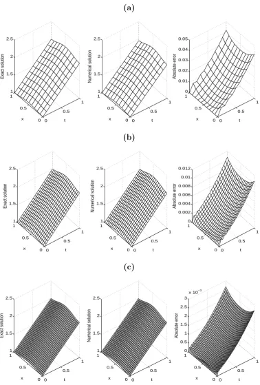
The grid convergence of the above FDM is considered next for solving the direct Neumann problem (1)–(3) with T =L= 1, and input data

φ(x) = u(x,0) = x2(x₋1)2+ 1, (42)

f(t) = 1

1 +t, g(x) =

−2 + 12x₋12x2

1 +x2_−2x3_+x4. (43)

The analytical solution for the temperature is given by

u(x, t) = x2(x₋1)2+ 1(1 +t). (44)

(a) 0 0.5 1 0 0.5 1 1 1.5 2 2.5 t x Exact solution 0 0.5 1 0 0.5 1 1 1.5 2 2.5 t x Numerical solution 0 0.5 1 0 0.5 1 0 0.01 0.02 0.03 0.04 0.05 t x Absolute error (b) 0 0.5 1 0 0.5 1 1 1.5 2 2.5 t x Exact solution 0 0.5 1 0 0.5 1 1 1.5 2 2.5 t x Numerical solution 0 0.5 1 0 0.5 1 0 0.002 0.004 0.006 0.008 0.01 0.012 t x Absolute error (c) 0 0.5 1 0 0.5 1 1 1.5 2 2.5 t x Exact solution 0 0.5 1 0 0.5 1 1 1.5 2 2.5 t x Numerical solution 0 0.5 1 0 0.5 1 0 0.5 1 1.5 2 2.5 3

x 10−3

t x

Absolute error

Figure 1: The exact (44) and numerical solutions for the temperatureu(x, t), with various mesh sizes (a) M = N = 10, (b) M = N = 20, and (c) M = N = 40, for the direct problem. The absolute error between them is also included.

Figure 2 with the exact solutions given by

β(t) = u(X0, t) = 17

16(1 +t), ψ(x) =u(x, T) = 2

x2(x₋1)2+ 1,

T = 1, X0 = 1

2. (45)

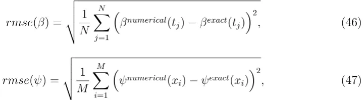
From Figure 2 it can be seen that the numerical solutions converge to the corresponding exact solutions (45), as the FDM grid becomes finer. In fact, the root mean square errors (rmse) defined by

rmse(β) =

v u u t

1 N

N X

j=1

βnumerical_(tj)−βexact_(tj)2_{, (46)}

rmse(ψ) =

v u u

t 1

M M X

i=1

ψnumerical_(xi)−ψexact_(xi)2_{, (47)}

indicated in Table 1, show more clearly their decreases as the grid size becomes smaller.

(a)

0 0.1 0.2 0.3 0.4 0.5 0.6 0.7 0.8 0.9 1

1 1.2 1.4 1.6 1.8 2 2.2 2.4

t

β

(t)

Exact solution M=N=10 M=N=20 M=N=40

(b)

0 0.1 0.2 0.3 0.4 0.5 0.6 0.7 0.8 0.9 1

1.9 1.95 2 2.05 2.1 2.15

x

ψ

(x)

Exact solution M=N=10 M=N=20 M=N=40

Table 1: The (rmse) given by equations (46) and (47) for β(t) and ψ(x), with various mesh sizesM =N _{∈ {}10,20,40_}, for the direct problem.

M =N 10 20 40

rmse(β) rmse(ψ)

0.0179 0.0374

0.0044 0.0094

0.0011 0.0024

4

Numerical approach to solve the inverse problem

In this section, we wish to obtain simultaneously the unknown functionsf(t) andg(x) in the inverse problem (1)–(7) reformulated as minimizing the regularized objective function

F(f, g) = _ku(x, T)₋ψ(x)_k2+_ku(X0, t)−β(t)k2+β1kf(t)k2+β2kg(x)k2

+ (g(X1)−α)2, (48)

whereusolves (1)–(3) for givenf andg, β1 ≥0 andβ2 ≥0 are regularization parameters, and the norm is usually theL2_{-norm. Assuming, for convenience, that we takeX}

0 ∈(0, L) such that there exists i0 ∈ {1, ..., M}for which X0 =xi0, in discrete form (48) becomes

F(f,g) = L

M M X

i=1 i6=i0

h

u(xi, T)₋ψ(xi)i2+ T N

N X

j=1 h

u(X0, tj)−β(tj) i2

+ (g(X1)−α)2

+β1 N X

j=1

f_j2+β2 M X

i=1

g_i2. (49)

The value fori =i0 in the first sum has been excluded in order to avoid duplicating the compatibility condition (in (7))u(X0, T) =u(xi0, T) =β(T) =β(tN) =ψ(xi0) = ψ(X0). The minimization of (49) is performed using the MATLAB toolbox routinelsqnonlin, which does not require the user to supply the gradient of the objective function, (Math-works, 2012). This routine attempts to find the minimum of a sum of squares by starting from arbitrary initial guessesf(0)_,g(0) _{forf,g,respectively. We have compiled this routine} with the following parameters:

• Algorithm = Trust-Region-Reflective (TRR), (Coleman and Li, 1996).

• Maximum number of iterations, (MaxIter) = 400.

• Maximum number of objective function evaluations, (MaxFunEvals) = 102_×(number of variables.)

• Termination tolerance on the function value, (TolFun) = 10−20_.

• x Tolerance, (xTol) = 10−20_.

The inverse problem under investigation is solved subject to both exact and noisy data which are numerically simulated as

βǫ1_{(tj) =β(tj) +ǫ1}

j, j = 1, N , (50)

ψǫ2_{(xi) = ψ(xi) +ǫ2i, i= 1, M , i}

6

=i0, (51)

where ǫ1j and ǫ2i are random variables generated from Gaussian normal distributions with mean zero and standard deviationsσ1 and σ2 given by

σ1 =p_× max

t∈[0,T]|β(t)|, σ2 = p×xmax∈[0,L]|ψ(x)|, (52)

where p represents the percentage of noise. We use the MATLAB function normrnd to generate the random variablesǫ1 = (ǫ1j)j=1,N and ǫ2 = (ǫ2i)_i=1,(M−1) given by

ǫ1 = normrnd(0, σ1, N), ǫ2 = normrnd(0, σ2, M ₋1). (53)

5

Numerical results and discussion

In this section, we present examples in order to test the accuracy and stability of the numerical methods introduced in Sections 3 and 4, respectively. The root mean square errors (rmse) are used to evaluate the accuracy of the numerical results and are defined by

rmse(f) =

v u u t

1 N

N X

j=1

fnumerical_(tj)−fexact_(tj)2_{, (54)}

rmse(g) =

v u u

t 1

M M X

i=1

gnumerical_(xi)−gexact_(xi)2_{. (55)}

In all examples we take, for simplicity, T = 1, L = 1 and X0 = X1 = L/2 = 0.5. Consequently, i0 =M/2 in (49). In all the inverse calculations we take M =N = 40.

5.1 Example 1

We solve the inverse problem (1)–(7) with unknown coefficients f(t) and g(x) and the input data (42), (45) and α = g(0.5) = 16/17. From this data one can observe that the conditions of Proposition 1 of Section 2 are satisfied and hence the inverse problem has a unique solution given by (10)–(12) which yield the expressions (43) and (44). We take the inital guess as

f0(t) = 1₋ t 2, g

0_{(x) =} (

−2 + 100

17x, 0≤x≤0.5, 66

17− 100

17x, 0.5< x≤1,

(56)

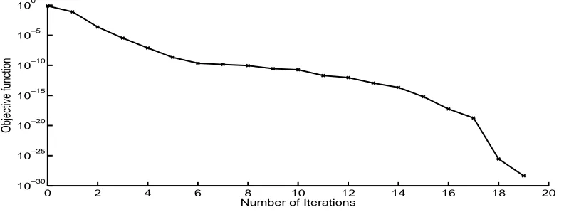
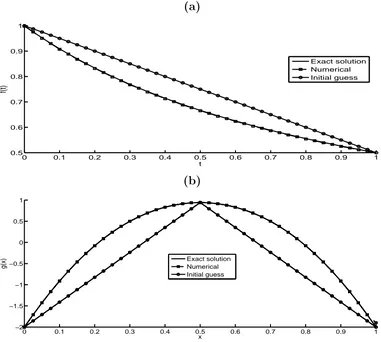
shows a rapid decrease to a low value of O(10−29_{) in 19 iterations. Figure 4 shows the} exact and numerical solutions of the functions f(t) and g(x), respectively. From this figure it can be seen that very accurate numerical solutions are obtained.

0 2 4 6 8 10 12 14 16 18 20

10−30 10−25 10−20 10−15 10−10 10−5 100

Number of Iterations

Objective function

Figure 3: Objective function (49) for Example 1 with no noise and no regularization.

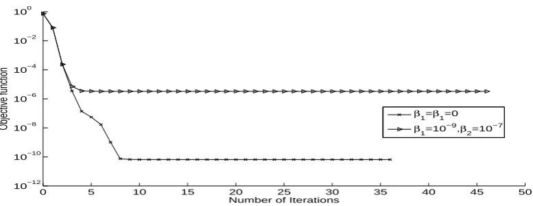
Next, we add a small amount ofp= 0.01% noise to the measured data (4) and (5). For higher amounts of noise the numerical results were less accurate and therefore they are not presented. The point to stress here is that since the inverse problem is ill-posed then we expect that regularization is needed in order to achieve stable and accurate results. The monotonic decreasing convergence of the objective function (49), as a function of the number of iterations, is shown in Figure 5 with and without regularization. Figure 6 shows the graphs of the recovered functions. From Figure 6 it can be seen that, as expected, when β1 = β2 = 0 we obtain unstable and inaccurate solutions because the problem is ill-posed and very sensitive to noise. Thus regularization is needed in order to stabilise the solutions. We selected by trial and error the regularization parametersβ1 = 10−9 and β2 = 10−7 which give stable and reasonable accurate solutions for the functions f(t) and g(x). For more elaborate choices of multiple regularization parameters, see (Belge et al., 2002; Fornasier et al., 2014).

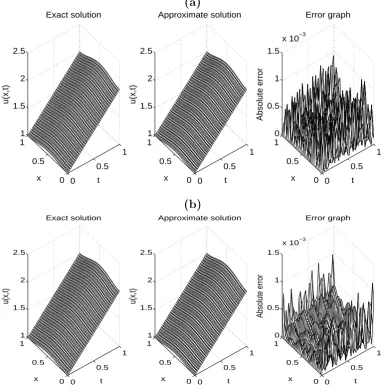
The related numerical results for the temperature u(x, t) with p = 0.01% noise, and with and without regularization, are presented in Figure 7 showing good agreement with the exact solution (44).

(a)

0 0.1 0.2 0.3 0.4 0.5 0.6 0.7 0.8 0.9 1

0.5 0.6 0.7 0.8 0.9 1

t

f(t)

Exact solution Numerical Initial guess

(b)

0 0.1 0.2 0.3 0.4 0.5 0.6 0.7 0.8 0.9 1

−2 −1.5 −1 −0.5 0 0.5 1

x

g(x)

Exact solution Numerical Initial guess

Figure 4: (a) Coefficient f(t) and (b) coefficient g(x), for Example 1 with no noise and no regularization.

Table 2: Number of iterations, number of function evaluations, value of the objective func-tion (49) at final iterafunc-tion, rmse(f) and rmse(g), and computational time, for Example 1.

Numerical outputs p= 0

(β1 =β2 = 0)

p= 0.01% (β1 =β2 = 0)

p= 0.01%

(β1 = 10−9, β2 = 10−7) Number of iterations

Number of function evaluations Value of objective function (49) at final iteration rmse(f)

rmse(g)

Computational time (sec)

19 1660 4.4E-29

0.0013 0.0156 163

36 3071 6.5E-11

0.1454 0.6698 306

46 3901 3.2E-6

0 5 10 15 20 25 30 35 40 45 50 10−12

10−10 10−8 10−6 10−4 10−2 100

Number of Iterations

Objective function

β

1=β1=0

β₁=10−9_,β 2=10

−7

Figure 5: Objective function (49), for Example 1 with p = 0.01% noise, with and without regularization.

(a)

0 0.1 0.2 0.3 0.4 0.5 0.6 0.7 0.8 0.9 1

0.2 0.4 0.6 0.8 1 1.2 1.4 1.6

t

f(t)

Exact solution

β₁=β₁=0

β₁=10−9,β₂=10−7 Initial guess

(b)

0 0.1 0.2 0.3 0.4 0.5 0.6 0.7 0.8 0.9 1

−4 −3 −2 −1 0 1 2

x

g(x)

Exact solution β₁=β₁=0 β₁=10−9,β

2=10 −7

Initial guess

(a) 0 0.5 1 0 0.5 1 1 1.5 2 2.5 t Exact solution x u(x,t) 0 0.5 1 0 0.5 1 1 1.5 2 2.5 t Approximate solution x u(x,t) 0 0.5 1 0 0.5 1 0 0.5 1 1.5

x 10−3

t Error graph x Absolute error (b) 0 0.5 1 0 0.5 1 1 1.5 2 2.5 t Exact solution x u(x,t) 0 0.5 1 0 0.5 1 1 1.5 2 2.5 t Approximate solution x u(x,t) 0 0.5 1 0 0.5 1 0 0.5 1 1.5

x 10−3

t Error graph

x

Absolute error

Figure 7: The exact and approximate solutions for the temperatures u(x, t), for Example 1, with (a) β1 =β2 = 0 and (b) β1 = 10−9, β2 = 10−7, for p = 0.01% noise. The absolute error

between them is also included.

5.2 Example 2

Consider the inverse problem (1)–(7) with the input data

φ(x) =u(x,0) = 2 + cos(πx), (57)

β(t) = u(0.5, t) = 2e t

2

1+t, ψ(x) = u(x,1) = √e(2 + cos(πx)), α=g(0.5) = 0. (58)

As in Example 1, the conditions of Proposition 1 are satisfied and the unique solution of the inverse problem (1)–(7) is given by (10)–(12) which yield

f(t) = t(t+ 2)

(t+ 1)2, g(x) =

π2_cos(πx)

2 + cos(πx), (59)

u(x, t) =e t

2

We take the inital guess as

f0(t) = 0, g0(x) =

( π2

3 −

2π2

3 x, 0≤x≤0.5,

π2_−2π2_{x, 0.5< x≤1.} (61)

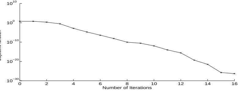
Analogous quantities and conclusions to Figures 3–6 and Table 2 of Example 1 are pre-sented and obtained in Figures 8–11 and Table 3 of Example 2.

0 2 4 6 8 10 12 14 16

10−30 10−20 10−10 100 1010

Number of Iterations

Objective function

Figure 8: Objective function (49), for Example 2 with no noise and no regularization.

(a)

0 0.1 0.2 0.3 0.4 0.5 0.6 0.7 0.8 0.9 1

−0.1 0 0.1 0.2 0.3 0.4 0.5 0.6 0.7 0.8

t

f(t)

Exact solution Numerical Initial guess

(b)

0 0.1 0.2 0.3 0.4 0.5 0.6 0.7 0.8 0.9 1

−10 −8 −6 −4 −2 0 2 4

x

g(x) _{Exact solution}

Numerical Initial guess

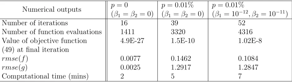
Table 3: Number of iterations, number of function evaluations, value of the objective func-tion (49) at final iterafunc-tion, rmse(f) and rmse(g), and computational time, for Example 2.

Numerical outputs p= 0

(β1 =β2 = 0)

p= 0.01% (β1 =β2 = 0)

p= 0.01%

(β1 = 10−12, β2 = 10−11) Number of iterations

Number of function evaluations Value of objective function (49) at final iteration rmse(f)

rmse(g)

Computational time (mins)

16 1411 4.9E-27

0.0077 0.0025 2

39 3320 1.5E-10

0.1462 1.2917 5

52 4316 1.02E-8

0.1084 1.2847 7

0 10 20 30 40 50 60

10−10 10−8 10−6 10−4 10−2 100 102

Number of Iterations

Objective function

β1=β1=0

β₁= 10−12,β

2= 10 −11

(a)

0 0.1 0.2 0.3 0.4 0.5 0.6 0.7 0.8 0.9 1

−0.2 0 0.2 0.4 0.6 0.8 1 1.2

t

f(t)

Exact solution

β₁=β

1=0

β₁= 10−12,β₂= 10−11 Initial guess

(b)

0 0.1 0.2 0.3 0.4 0.5 0.6 0.7 0.8 0.9 1

−15 −10 −5 0 5

x g(x) Exact solution

β₁=β₁=0

β₁=10−12,β₂= 10−11 Initial guess

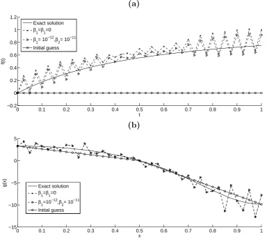
Figure 11: (a) Coefficient f(t) and (b) coefficient g(x), for Example 2 with p = 0.01% noise, with and without regularization.

5.3 Example 3

The previous examples possessed an analytical solution available for the triplet

(u(x, t), f(t), g(x)). In this section, we investigate an example for which an analytical solution for u(x, t) is not available. We take the initial condition (2) given by

u(x,0) =φ(x) =



  

  

1, 0_≤x <1/4, 5

4 −x, 1/4< x≤1/2, x+ 1₄, 1/2< x_≤3/4, 1, 3/4< x_≤1,

(62)

which represents a non-smooth function. In the absence of an analytical solution for u(x, t) being available we generate the input data (4) and (5) numerically by solving first the direct problem given by (1)–(3) with φ(x) given by (62), and the known functions

f(t) = 1 +t, g(x) = 1 +x, (63)

using the FDM described in Section 3.

The example considered in this subsection violates the sufficient conditions of unique-ness of solution of Proposition 1 and (Savateev, 1995) and therefore, it is a severe test for our method of regularization.

In order to avoid committing an inverse crime the mesh that is used for numerically simulating the measured data (4) and (5) by solving the direct problem is taken to be more dense than the one used for the solution of the inverse problem, (Kaipio and Somersalo, 2007). Consequently, in the inverse problem we use the FDM withM =N = 40 and half of the data forβ and ψ obtained from solving the direct problem withM =N = 80. We also take the initial guess as

f0(t) = 1, g0(x) = 1. (64)

The objective function (49) with no noise and no regularization, as a function of the number of iterations, is plotted in Figure 13. From this figure it can be seen that a rapid monotonic decreasing convergence to a low value of O(10−28_{) is achieved in about 12} iterations.

(a)

0 0.1 0.2 0.3 0.4 0.5 0.6 0.7 0.8 0.9 1

0 5 10 15 20

t

β

(t)

M=N=20 M=N=40 M=N=80

(b)

0 0.1 0.2 0.3 0.4 0.5 0.6 0.7 0.8 0.9 1

18 18.5 19 19.5 20

x

ψ

(x)

M=N=20 M=N=40 M=N=80

Figure 12: The numerically convergent solutions for (a)β(t) and (b)ψ(x), for Example 3 with various mesh sizesM =N _{∈ {}20,40,80_} for the direct problem.

0 2 4 6 8 10 12 10−30

10−20 10−10 100 1010

Number of Iterations

Objective function

Figure 13: Objective function (49), for Example 3 with no noise and no regularization.

(a)

0 0.1 0.2 0.3 0.4 0.5 0.6 0.7 0.8 0.9 1

0.8 1 1.2 1.4 1.6 1.8 2

t

f(t)

Exact solution Final iteration Initial guess

(b)

0 0.1 0.2 0.3 0.4 0.5 0.6 0.7 0.8 0.9 1

0.8 1 1.2 1.4 1.6 1.8 2

x

g(x)

Exact solution Final iteration Initial guess

Figure 14: (a) Coefficient f(t) and (b) coefficient g(x), for Example 3 with no noise and no regularization.

Finally, details about the number of iterations, the rmse(f) and rmse(g) in (54) and (55), respectively, and the computational time, are given in Table 4 for various values of the regularization parameters β1 = β2. For p = 1% noise and no regularization the computational time and the number of iterations increase drastically and the rmse(f) and rmse(g) become very large, which is expected due to the instability of the inverse and ill-posed problem. However, as previously obtained from Figure 16, it can be seen that accurate and stable numerical results are achieved if regularization is employed.

0 5 10 15 20 25 30 35 40 45

10−4

10−2

100

102

104

Number of iterations

Regularized objective function

β

1=β2=10 −5

β

1=β2=10 −3

β₁=β

2=10 −2

(a)

0 0.1 0.2 0.3 0.4 0.5 0.6 0.7 0.8 0.9 1

1 1.5 2 2.5

t

f(t)

Exact solution

β₁=β₂=10−5

β₁=β

2=10 −3

β₁=β₂=10−2

(b)

0 0.1 0.2 0.3 0.4 0.5 0.6 0.7 0.8 0.9 1

1 1.5 2 2.5

x

g(x)

Exact solution

β₁=β

2=10 −5

β₁=β₂=10−3

β₁=β₂=10−2

Table 4: Number of iterations, computational time, and rmse values for p _∈ {0.01,0.1,1_}% noise, with and without regularization, for Example 3.

p Regularization rmse(f) rmse(g) Iter Time

0.01%

β1 =β2 = 0 β1 =β2 = 10−5 β1 =β2 = 10−4 β1 =β2 = 10−3 β1 =β2 = 10−2 β1 =β2 = 10−1

0.3373 0.0406 0.0525 0.0613 0.0899 0.1831 0.5775 0.0658 0.0448 0.0403 0.0494 0.1180 18 42 41 38 41 41 3 mins 4 mins 5 mins 6 mins 5 mins 5 mins

0.1%

β1 =β2 = 0 β1 =β2 = 10−5 β1 =β2 = 10−4 β1 =β2 = 10−3 β1 =β2 = 10−2 β1 =β2 = 10−1

3.3704 0.2458 0.1018 0.0678 0.0909 0.1830 5.7759 0.3619 0.0895 0.0335 0.0466 0.1197 47 47 39 39 50 50 8 mins 8 mins 6 mins 6 mins 9 mins 9 mins 1%

β1 =β2 = 0 β1 =β2 = 10−5 β1 =β2 = 10−4 β1 =β2 = 10−3 β1 =β2 = 10−2 β1 =β2 = 10−1

35.9469 2.5250 0.9086 0.2720 0.1139 0.1820 53.9733 3.5760 0.7765 0.1581 0.0527 0.1366 401 50 47 50 38 50 1 hour 9 mins 8 mins 9 mins 6 mins 9 mins

6

Conclusions

This paper has presented the determination of an additive time and space-dependent per-fusion coefficient from data measurements in the one-dimensional parabolic heat equation. The direct solver based on a Crank-Nicolson finite difference scheme was employed. The resulting inverse problem has been reformulated as a constrained regularized minimization problem which was solved using the MATLAB optimization toolbox routine lsqnonlin. The numerically obtained results are stable and accurate.

Future work will concern inversion of real physical temperature data (4) and (5) to reconstruct the additive time- and space-dependent perfusion coefficient in the context or bio-heat transfer, (Lesnic and Trucu, 2010) or the heat transfer coefficient in the context of fins used in condensers and evaporators, (Marinet al., 2004).

Acknowledgments

M.J. Huntul would like to thank Jazan University in Saudi Arabia and United Kingdom Saudi Arabian Cultural Bureau (UKSACB) in London for supporting his PhD at the University of Leeds.

References

reg-1161–1183.

[2] Coleman, T.F. and Li, Y. (1996) An interior trust region approach for nonlinear minimization subject to bounds,SIAM Journal on Optimization, 6, 418–445.

[3] Deng, Z.C., Yang, L., Yu, J.N. and Luo, G.W. (2010) Identifying the radiative co-efficient of an evolutional type heat conduction equation by optimization method,

Journal of Mathematical Analysis and Applications, 362, 210–223.

[4] Deng, Z.C., Yu, J.N. and Yang, L. (2008) Optimization method for an evolutional type inverse heat conduction problem,Journal of Physics A: Mathematical and The-oretical,41, 035201, (20 pp).

[5] Fornasier, M., Naumova, V. and Pereverzyev, S.V. (2014) Parameter choice strategies for multipenalty regularization, SIAM Journal on Numerical Analysis, 52, 1770– 1794.

[6] Hazanee, A. and Lesnic, D. (2013) Reconstruction of an additive space- and time-dependent heat source,European Journal of Computational Mechanics,22, 304–329.

[7] Hao Dinh Nho, Thanh Phan Xuan, Lesnic, D. and Ivanchov, M. (2014) Determination of a source in the heat equation from integral observations,Journal of Computational and Applied Mathematics, 264, 82–98.

[8] Kaipio, J. and Somersalo, E. (2007) Statistical inverse problems: discretization, model reduction and inverse crimes, Journal of Computational and Applied Math-ematics,198, 493–504.

[9] Lewis, R.W., White, I.R. and Wood, W.L. (1978) A starting algorithm for the nu-merical simulation of two-phase flow problems, International Journal for Numerical Methods in Engineering, 12, 319–329.

[10] Lesnic, D. and Trucu, D. (2010) The identification of blood perfusion coefficient in bio-heat transfer, Inverse Problems, Design and Optimization Symposim (IPDO-2010), Joao Pessoa, Brazil, CD-ROM, pp. 277-284.

[11] Marin, L., Elliott, L., Heggs, P.J., Ingham, D.B., Lesnic, D. and Wen, X. (2004) Analysis of polygonal fins using the boundary element method, Applied Thermal Engineering,24, 1321–1339.

[12] Mathworks (2012) Documentation Optimization Toolbox-Least Squares (Model Fit-ting) Algorithms, available at www.mathworks.com/help/toolbox/optim/ug

/brnoybu.html.

[13] Samarskii, A.A. and Vabishchevich, P.N. (2007) Numerical Methods for Solving Inverse Problems of Mathematical Physics, De Gruyter, Berlin.

[14] Savateev, E.G. (1995) On the problem of identification of a coefficient in a parabolic equation.Siberian Mathematical Journal, 36, 177–185.

[16] Trucu, D., Ingham, D.B. and Lesnic, D. (2008) Inverse time-dependent perfusion coefficient identification,Journal of Physics: Conference Series: 4th AIP Internatinal Conference and the 1st Congress of the IPIA, 124, 012050, (28 pages).

[17] Trucu, D. (2009) Inverse Problems for Blood Perfusion Identification, PhD Thesis, University of Leeds.

[18] Trucu, D., Ingham, D.B. and Lesnic, D. (2010) Space-dependent perfusion coefficient identification in the transient bio-heat equationJournal of Engineering Mathematics,

67, 307–315.

[19] Trucu, D., Ingham, D.B. and Lesnic, D. (2011) Reconstruction of the space- and time-dependent blood perfusion coefficient in bio-heat transfer,Heat Transfer Engineering,

32, 800–810.