This is a repository copy of
Motion anomaly detection and trajectory analysis in visual
surveillance
.
White Rose Research Online URL for this paper:
http://eprints.whiterose.ac.uk/120854/
Version: Accepted Version
Article:
Chebiyyam, M., Reddy, R.D., Dogra, D.P. et al. (2 more authors) (2017) Motion anomaly
detection and trajectory analysis in visual surveillance. Multimedia Tools and Applications.
ISSN 1380-7501
https://doi.org/10.1007/s11042-017-5196-6
[email protected] https://eprints.whiterose.ac.uk/
Reuse
Items deposited in White Rose Research Online are protected by copyright, with all rights reserved unless indicated otherwise. They may be downloaded and/or printed for private study, or other acts as permitted by national copyright laws. The publisher or other rights holders may allow further reproduction and re-use of the full text version. This is indicated by the licence information on the White Rose Research Online record for the item.
Takedown
If you consider content in White Rose Research Online to be in breach of UK law, please notify us by
Reddy · Debi Prosad Dogra · Harish
Bhaskar · Lyudmila Mihaylova
Received: / Accepted:
Abstract Motion anomaly detection through video analysis is important for delivering autonomous situation awareness in public places. Surveillance scene segmentation and representation is the preliminary step to implementation anomaly detection. Surveillance scene can be represented using Region Asso-ciation Graph (RAG), where nodes represent regions and edges denote con-nectivity among the regions. Existing RAG-based analysis algorithms assume simple anomalies such as moving objects visit statistically unimportant or abandoned regions. However, complex anomalies such as an object encircles within a particular region (Type-I) or within a set of regions (Type-II). In this paper, we extract statistical features from a given set of object trajectories and train multi-class support vector machines (SVM) to deal with each type of anomaly. In the testing phase, a given test trajectory is categorized as nor-mal or anonor-malous with respect to the trained models. Performance evaluation of the proposed algorithm has been carried out on public as well as our own datasets. We have recorded sensitivity as high as 86% and fall-out rate as low as 9% in experimental evaluation of the proposed technique. We have car-ried out comparative analysis with state-of-the-art techniques to benchmark the method. It has been observed that the proposed model is consistent and highly accurate across challenging datasets.
Keywords Visual surveillance, Anomalous activity detection, Abnormal behavior classification, Trajectory analysis.
M. Chebiyyam, R. D. Reddy, D. P. Dogra
School of Electrical Sciences, IIT Bhubaneswar, India E-mail:{mbc10, rrd10, dpdogra}@iitbbs.ac.in
H. Bhaskar
Department of Computer Science and Engineering, Khalifa University, U.A.E E-mail: [email protected]
L. Mihaylova
1 Introduction
Learning-based methods have boosted autonomous analysis of high-dimensional spatio-temporal video data. Conventional visual analysis requires integration of statistical inference with computational models. Advances in capability of object localization, recognition, and tracking in videos have allowed researchers to think of designing autonomous decision making systems in situation aware-ness applications.
CCTV-based video surveillance has emerged lately and being given more priority for national security in developing countries. Modern development in autonomous surveillance has surpassed the legacy of requiring human adminis-trators to examine several hours of visual feed [1] to summarize socio-economic scenarios [2] or mining critical forensic evidences [3]. This has been widely supported by the growth of video analytic capabilities in applications such as motion detection [4, 5], tracking [6], parsing [7], activity recognition [8], behavioural understanding [2, 3, 9], traffic analysis [10], parking area monitor-ing [11], abandoned object detection [12, 13], suspicious activity detection [14], and scene understanding [15]. With rapid developments in autonomous visual surveillance, such analytic systems are becoming highly prevalent in environ-ments such as airports, shopping malls, railway stations and subways in mod-ern smart cities.
One of the key steps towards complete situation awareness is anomalous activity detection. The objective is to determine if visually perceived move-ments of objects can be categorized as normal or abnormal. This can be used to detect compromise in security. However, what constitutes an abnormal or anomalous motion has remained a topic of debate. While providing a formal definition of anomalous activity seems subjective, its quantification is even more complex. Several behavioural analysis methods have been introduced re-cently within the visual surveillance domain [16–18]. A major share of these studies build models over the visual perception of target motion and quantifies them based on motion characteristics, thus recognizing anomalous activities. In this context, pattern recognition and machine learning guided techniques to understand and comprehend target motion through trajectory analysis, is gaining significance.
back-in temporal domaback-in, where each segment can be classified back-into a different category of interest [3, 40]. In such algorithms, the overall change in scene dy-namics within any chosen time interval is considered as an important feature towards identifying a temporal segment of interest. Any measured deviations from these supervised segments of interest is often classified anomalous [8]. Anomaly detection can be performed at holistic as well as individual levels. While the holistic viewpoint addresses variations among clustered trajecto-ries within a scene, individual trajectotrajecto-ries can also be analysed to determine video segments containing possible anomalous motion. However, such meth-ods compute statistical mean of trajectories during training and use them as a reference to find deviation from normal class centroids. These methods are popular in visual surveillance applications [41, 42]. More recently, Brun et al. [11, 15] have proposed a scene partitioning approach to classify trajectories using unsupervised learning. Main idea in their method is to divide the scene into non-overlapping zones and to represent it using a graphical structure sim-ilar to the method proposed in [43]. Brun et al. have clustered car trajectories recorded from parking zones [44] and human trajectories obtained inside a busy railway station [45]. The method proposed in [43] has been used to de-tect very simple anomalies such as a target visiting abandoned or inaccessible regions. Further, a similar method, often refereed as non-conformal recognition technique has also been recently introduced for maritime applications [46]. Ac-cording to [46], a conformal anomaly prediction method using a kernel-density estimation based non-conformal measure has been applied to detect suspicious behaviours of ships due to sudden changes in direction, speed or anchoring. In another study, a Sequential Hausdorff Nearest-Neighbour Conformal Anomaly Detector (SHNN-CAD) has been proposed by [47] for online learning and se-quential anomaly detection using motion trajectories. Despite the algorithm being parameter-light, the performance of the technique in [47] is highly influ-enced by the learning procedure and the choice of training set.
different datasets. In another study by [49], the classification of the visual scene into dominant versus rare activities using spatio-temporal models and local similarity has been addressed. Activity detection in other domains have also attracted researchers. For example, Liu et al. [50–54] have proposed a handful of methods to detect human activities during various types of interac-tions. The method in [49] engages the Histogram of Oriented Gradient (HOG) features within an online Fuzzy C-Means clustering technique for behaviour understanding. In a similar study by [55], several local descriptors have been used in conjunction with spatio-temporal filtering and local k-nearest neigh-bour algorithm for composite training and detection of motion anomalies in video. The local features explored within the work of [55]include persistence, direction and motion magnitude. Finally, the use of spatio-temporal context analysis for the accurate anomalous event detection and localization has been proposed in [56]. Context-aware anomalous activity detection has also been studied in [43, 57]. Here, it has been demonstrated that in order to deter-mine scene dynamics that relate to target interactions, it is critical to analyze the target motion saliency for reliable anomalous activity detection. For ex-ample, if a target deviates from its normal path or spends additional time within a confined area of interest, the dynamics need not necessarily suggest anomalous activity. The activity may be normal depending on the context. For example, a predefined place within the viewing field may be one of the region(s)-of-interest, where people usually visit and stays for longer duration. Thus, contextual information plays a vital role in deciding anomalous activi-ties.
Despite recent developments in this research domain, the problem of motion anomaly detection still remains to be challenging due to the following reasons: a) To identify what constitutes anomalous within the surveillance context and distinguishing it from normal behaviour, b) To propose a scene independent model that can work under varying scene conditions, c) To deal with the complexity in behavioural patterns of moving targets, and d) To operate within reasonable computational overhead. Majority of the above mentioned state-of-the-art methodologies do not address the first challenge, whereas the method proposed in [43] has been shown to handle very simple motion anomalies. Although the unsupervised approach proposed by Burn et al. [11, 15] can successfully classify trajectories, this method does not provide any insight on the type and category of the anomaly. In addition to that, threshold-based classification approach adopted in [11] may not be applicable under varying environmental conditions.
1.2 Contributions of the Paper
– Validation of the proposed methodology on publicly available challenging datasets and our dataset and providing a comparative analysis with state-of-the-art techniques in this field of study.
The rest of the paper is organized as follows. In Section 3, the detailed methodology of the proposed solution is described. Results and discussions are illustrated in Section 4. Finally, Section 5 concludes the paper.
2 Proposed Methodology
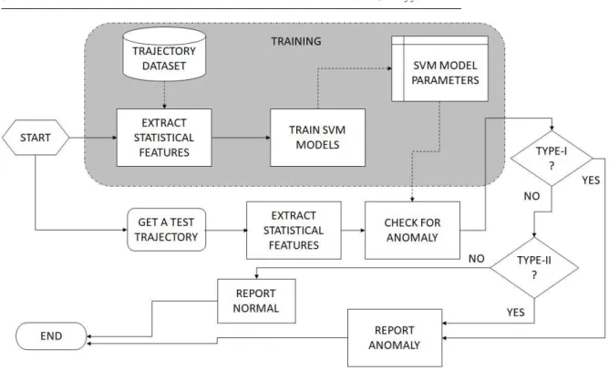
We present our proposed anomaly detection framework in Fig. 1. The proposed anomaly detection technique operates in two phases, training and testing. In the training phase, support vector machines are trained using the statistical features extracted from a given set of trajectories. Therefore, when the scene is changed, we carry out the training of SVM parameters using the new set of trajectories available. During testing, a trajectory is verified against the trained models. Testing of a trajectory is instanteneous and whenever a given test trajectory violetes the statistical model, we generate the alarm. Statistical feature extraction has been carried out using a method proposed in [43]. These steps are described in the following sections.
2.1 Importance-based Scene Segmentation
Consider that a visual surveillance scene at a given instance of time, captured from a CCTV camera, is represented as an image frame I. Given the scene
I and a set of trajectories ∆ of moving targets inside that scene, the aim is to build a segmentation map S composed of homogeneous regions, where-in the criterion of homogeneity is based on the importance of each region within that scene. Assuming that the original sceneIis uniformly divided into rectangular blocksb, the aim is to decomposeIintoKnumber of semantically homogeneous regions each of which is identified by the region-correspondence variableRb∈1, ..., K. Here, therthregion is the set of blocksBr, whose region
correspondence variable equals r, i.e., Br = {b : Rb = r}. The problem of
Fig. 1: Flowchart of the proposed anomaly detection algorithm.
I≃[
r Br=
[
b
{b:Rb=r} ∈1, ..., K =S. (1)
Rb=argmax
− →
f(−→b). (2)
∀bf(b) = (ib). (3)
where, −→f(−→b) represents motion dynamics features extracted from each indi-vidual block that is based on the measurement of an importance criterionib.
Further, blocks with similar importance (ib) are clustered together in order to
build homogeneous-regions within the scene. The importance criterion corre-sponding to each block is based on motion dynamics features including the velocity of targets within each block and the overall time spend by the target while visiting the block, i.e.
ib=∀b ρb gb
. (4)
where, ρb represents the popularity index of the block b and is normalized
against the total number of times a block b is visited by different targets (represented asgb).
ρb=ρb+
vo−vo j
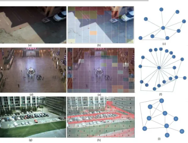
Fig. 2: (a-b) Segmentations of surveillance scenes (MIT and In-HOUSE datasets) using the method proposed in [43]. (c-d) Corresponding RAG rep-resentations of the scenes. For example, in (a) Green - mostly accessed blocks (L1), Blue - frequently visited blocks (L2), Red - rarely visited blocks (L3)
and Black/Gray - in-accessed blocks (L4).
Here, it is assumed that the instantaneous velocity (vo
j) of a target is
ex-pected to be lower than its average velocity (vo). Further to analyzing the importance distributions from different surveillance scenes, region-labels were chosen to be discretized into 4 classes{Rb:{1,2,3,4}}: interesting blocksL1
represented as the local maxima within the importance distribution, frequently visited blocksL2, rarely visited blocksL3 and in-accessed blocksL4.
A simple 8-connected component analysis is engaged for clustering the class labels indicating relative importance of blocks in order to generate ho-mogeneous regions. Two examples of the scene segmentation are illustrated in Fig. 2(a-b).
2.2 Scene Representation using RAG
In order to enable seamless inference on the segmented sceneS, a RAG rep-resented as G(V, E), where v ∈ V and e∈ E represents nodes and edges of the graph, is constructed. Each homogeneous region in the segmentation map
each vertexv(w) in the RAGGis estimated as follows. Assumezindependent trajectory segments pass through a vertex vi, then its weight vi(w) is
com-puted using (6), where sj is the length of the jthtrajectory segment passing
throughvi. Note that, nodes that are labeled in-accessible, are initialized with
zero weight,
vi(w) =
s1+s2+....+sz
z . (6)
The structure of the constructed RAG represents the overall connectivity of various regions that constitute a surveillance scene. Therefore, given a test trajectory recorded over the same scene, it is possible to benchmark this test trajectory against the RAG and hence categorize its motion into normal or anomaly class.
3 Motion Anomaly Detection
According to the proposed method described so far, a surveillance sceneIhas been shown to be transformed into a segmented sceneS represented using a weighted RAGG, based on motion dynamics features extracted from target trajectories. Some examples of the RAG representation of surveillance scenes are illustrated in Fig. 2(c-d). Although, the proposed method relies on localised importance estimated across blocks of regions; estimating importances using other low-level features such as the use of context [58], trajectory density [11, 15], motion [59, 60], spatio-temporal scene structure [61] are also possible.
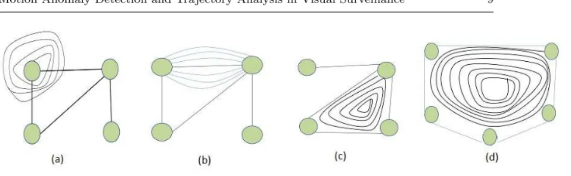
Fig. 3: Demonstration of possible representation of two types of anomalous situations described in this paper. (a) I anomalous situation. (b-d) Type-II anomalous situations.
3.1 Analysis of Type-I Anomaly
In this paper, a Type-I motion anomaly is classified based on the relationship between the motion characteristics of a target that appears within a region of the scene and the type (label) of region within the scene that the target visits. For example, if a target is found to have spent more than usual time within a region that has been previously labelled either as rarely visited (L3) or not
visited at all (L4), then Type-I anomaly is flagged. Here, the approach could
be to compare the test trajectory of a target to the statistical data acquired during training to determine deviations. This paper proposes a probabilistic approach to the classification of Type-I anomaly as defined below. Let a set of
κtraining trajectories {τ1, τ2, ..., τκ} be denoted using (7) and a surveillance
sceneIbe represented using a RAG, sayG(V, E), where (8) and (9) represent set of vertices{v1, v2, ..., vn}and edges{e1, e2, ..., eh}, respectively,
∆={τ1, τ2, τ3, ..., τκ}, (7)
V ={v1, v2, ...., vn}, (8)
E={e1, e2, ..., eh} (9)
Each vertex in the RAG represents one homogeneous region that has been labeled during training. An edge (e) between two vertices, is drawn if regions are adjacent. For a given RAG (G) and a set of training trajectories (∆) of targets within the surveillance scene, the probability p(vj|∆) of a target
visiting vertex (vj) is first estimated. Further, given an unknown trajectory, say τtest, the objective is to exploit the estimated probabilityp(vj|∆) as features
Akthtrajectory (τ
k) can be considered as a time-series data as given in (10),
where (ui, vi) pair denotes the location of the target at a given time instant.
τk ={(u1, v1),(u2, v2), ...,(uo, vo)} (10)
The first step is to transform the trajectory of the moving target repre-sented asτk into an equivalent path w.r.t the RAG generated from the scene.
Letρk denote the equivalent path ofτk coveringm vertices as given in (11),
where |vj| represents the duration of time spent by the target within vertex vj,
ρk= (v1,|v1|)→(v2,|v2|)→...→(vmk,|vmk|). (11)
Further, the probability of a moving target visiting a particular vertex in the RAG can be estimated using a set of paths. That is, given a set of trajectories (∆), it is possible to estimate the general probability of a target visiting vertex vj using (12), where |ρ
vj
i | and |ρi| represent the duration of
time spent by the target within vertexvj and total duration of its trajectory
(τi), respectively.
p(vj|∆) =
|ρvj
1 |+|ρ
vj
2 |+...+|ρ
vj
k |
|ρ1|+|ρ2|+...+|ρk|
(12)
Similarly, the probability of a target visiting a vertex vj according to its
own trajectory or path (ρi) can be estimated using (13)
p(vj|ρi) =
|ρvj
i |
|ρi|
. (13)
Equations (12) and (13) in combination can be used to prepare the training samples for classification. In the proposed approach, a separate classifier for each vertex is trained using the feature vector as given in (14) representing the trajectory path (ρi) with its corresponding label vector as represented
using (15),
Fρi = [|ρ
v1
i |,|ρ v2
i |, ...,|ρ vmi i |]
T
, (14)
Lρi = [l
v1
ρi, l
v2
ρi, ..., l
vmi ρi ]
T
, (15)
where
lvj
ρi =
+1 whenp(vj|ρi)≥β×p(vj|∆),
−1 whenp(vj|ρi)< β×p(vj|∆) (16)
whereβis a multiplication factor that determines the class of a given training trajectory with respect to all trajectories present in the training set. Based on the choice of β, data is prepared for training the classifiers. More precisely,
3.2 Analysis of Type-II Anomaly
As mentioned earlier, a target could visit several regions of a surveillance scene in different motion patterns. However, scenarios depicted in Figs. 3(b-d) can be considered as potential candidates for Type-II anomaly. It is clear that Type-II anomaly is more complex than Type-I anomaly. In contrast to Type-I anomaly, where finding the path within the RAG is critical, Type-II requires finding cycles in a path. Therefore, SVM classifiers are constructed for each candidate cycle in order to determine anomaly. Formally, the detection of Type-II anomaly shall exploit the probabilityp(cj|∆), wherecj represents aℓ
-cycle segment defined when a loop coveringℓdistinct nodes is identified from a given RAGGand a set of training trajectories (∆). Further, the objective is to use this probabilityp(cj|∆), for every possibleℓ-cycles present inGaccording
to a given training set∆to classify an unknown trajectoryτtestas anomalous
or normal.
However, detecting cycles of any length (closed walk or simple cycle) in a graph is a NP-complete problem. It has been shown in [62] that this problem can be solved in either O(V E) time or O(VωlogV) time when the length of
the cycle is knowna priori. Similarly, Flum and Grohe in [63] have shown that counting of cycles and paths of lengthℓin both directed and un-directed graphs is not NP-complete for a givenℓ. It has been proved that, when 3≤ℓ≤7, it is possible to count allℓ-cycles (a cycle that includesℓdistinct nodes) inO(Vω)
time. In order to alleviate the complexity of solving an NP-complete problem and for simplicity, in this paper, it has been chosen to restrict the search for cycles in the RAG to a maximum length of 4, i.e.,≤4.
Let,C={c1, c2, ..., cψ}denote a set of cycles of length≤4 present within
a given RAGG. Thus, a numberψof SVM classifiers are trained, one for each cycle using a set of training trajectories∆. However, the features required to train these classifiers are relatively more complicated than those used during Type-I anomaly analysis. In addition, searching forℓ-cycles from a given tar-get trajectory is also a hard problem. Although, a brute-force approach can be employed to solve this, such methods are not efficient and to process a large number of trajectories using this approach would not be computation-ally tractable. Therefore, the following mechanism has been adopted to find
A path, say ρi ∈ ∆, is initially represented using (11) with each vertex
expanded by its weight. For example, the path given in (11) can be expanded into ρi = (v1 → v1 → ... → v1)|v1| → (v2 → v2 → ... → v2)|v2| → ... →
(vm→vm→...→vm)|vm|, where a vertex in this expanded path is assigned a unique but non-linearly quantized label. Thus, Ψ non-linear quantization labels, e.g.q1, q2, ..., qΨ are selected to represent a path. Such an expansion
and non-linear quantization is necessary to determine sparsity of transitions between any pair of nodes. Now, given an expanded representation of the path, it can easily be differentiated fromqj in order to localize the transitions
between two nodes u and v. Because of using the non-linear quantization approach, ρi+1−ρi
qj−1−qj
can be used to unambiguously locate transitions between any pair of nodes. Once all such transitions have been identified, cycles can be localized by grouping transitions present within each path. By parsing the path for a contiguous re-appearances of similar transitions, only such desired transitions can be distinguished from others and extracted. In addition, while searching for cycles involving nodes, sayuandv, the sparsity in transitions is also checked and if found highly sparse, it is assumed that the path does not indicate any aberrant behavior.
In the proposed method, the frequency of transitions between any pair of nodes within a path is used to estimate the probability of transitions for a given target. Further, given a set of training trajectories (∆), transitions that represent similar repetitive cycles are marked, features are extracted and fed into the classifiers. Probabilistic measures similar to those introduced in (12) and (13) of Section 3.1 are used to train these classifiers. However, the esti-mation of general as well as individual probability values are done exclusively. Equations (17)-(18) illustrate the general probability of aℓ-cycle given all tra-jectories in the training dataset, whereλrepresents the minimum number of times a cyclecj must be repeated by a target in order to consider the
trajec-tory to be anomalous, γi represents those instances where cyclecj appeared
more than λtimes and ηi denotes the total number of times that the cycle
appeared within the whole dataset,
p(Xcj > λ|∆)
= γ1(Xcj > λ+ 1) +γ2(Xcj > λ+ 2) +...
η1(Xcj = 1) +η2(Xcj = 2) +... =p(Xcj =λ+ 1|∆) +p(Xcj =λ+ 2|∆) +....
(17)
where Xcj indicates the expected number of occurrences of the cyclecj in a given path,
p(Xcj =λ+r|∆) =
γ1(Xcj > λ+r+ 1)
η1(Xcj = 1) +η2(Xcj = 2) +...
. (18)
Similarly, the probability of a ℓ-cycle to appear in a particular path (ρi)
=p(Xcj =λ+ 1|ρi) +p(Xcj =λ+ 2|ρi) +....
such that,
p(Xcj =λ+r|ρi) =
ω1(Xcj > λ+r+ 1)
φ1(Xcj = 1) +φ2(Xcj = 2) +...
(20)
Equations (17) and (19) are used to prepare the training samples neces-sary for Type-II anomaly classification using ψclassifiers. A feature vector is constructed for each training trajectory with its corresponding label vector in a manner similar to that introduced for Type-I analysis.
Fρi = [|ρ
c1
i |,|ρ c2
i |, ...,|ρ cψ
i |] T
(21)
Lρi= [l
c1
ρi, l
c2
ρi, ..., l
cψ
ρi]
T. (22)
The corresponding label vector as given in (22) can be generated using (23)
lcj
ρi =
+1 whenp(Xcj > λ|ρi)≥β×p(Xcj > λ|∆)
−1 whenp(Xcj > λ|ρi)< β×p(Xcj > λ|∆)
. (23)
Finally, Equations (21)-(23) are used for training theψ classifiers, one for each cycle. Now, given a test trajectory or path (ρtest) as given in (24) can be
computed and used to testρtest against the ψclassifiers.
Fρtest = [|ρ
c1
test|,|ρ c2
test|, ...,|ρ cψ
test|] T
(24)
It is assumed that if at least one of the classifiers returned negative, then ρtest is considered abnormal. The mathematical formulation of
3.3 Classification
Prediction of unlabelled data is highly important in a typical classification problem. Researchers have used prediction-based techniques in various appli-cations [64–67]. The same logic applies to the present work. Since SVM is a well established predictor, it has been used for the classification of both Type-I and Type-II anomalies. SVM is a set of supervised learning methods used for classification, regression and outliers detection [68]. Though, SVM classifiers are best known for binary classification, however, it has also been used for multi-class separation [69]. With different kernel functions that can be specified for a decision function, SVM is widely used to find the optimal hyper-plane between two classes. In the proposed problem, Fρ from either
Type-I or Type-II anomaly is considered as the feature vector, fed as input
xto these SVM classifiers. The objective is to learn a classifier y =f(x, α), whereαare the parameters of the function using a linear kernel as the decision functionf(.). Given training data (xi, yi) fori= 1,2,3..., N with xi ≡Fρi andyi ∈ {−1,+1}, a typical 2-D linear classifier is of the form as given in (25),
where ,ǫis the normal to the line andbis the bias. Though,ǫis known as the weight vector, it can be learned by through [68]
f(xi) =ǫTxi+b. (25)
Using the perceptron algorithm, ǫ is initialized to 0. Then an iterative training is performed and Depending on the classification ofxiduring iterative
processing,ǫis updated using (26)
ǫ=ǫ+αsign(f(xi))xi. (26)
The training process is continued till all data points are correctly classified. At the end of training, final value ofǫis computed using (27)
ǫ=
N
X
i
αixi. (27)
However, the above training algorithm works only if the data is linearly separable. Finally, the line of classification can be determined using (28), where
xi’s are the support vectors of the classifier, i.e.
f(x) =X
i
αiyi(xTi x) +b (28)
SinceǫTx+b= 0 on the classifier,ǫis normalized such thatǫTx
++b= 1
andǫTx
−+b=−1 hold for positive and negative support vectors, respectively.
The margin between these support vectors is given as 2
||ǫ||. It is possible that
4 Experimental Results
In this section, experimental details and results that validate the performance of the proposed methodology and comparisons against the state-of-the-art us-ing various dataset are reported.
4.1 Description of Datasets
Three datasets including the Grand Central Station dataset (CUHK) [45], MIT trajectory dataset [44] and a custom-built in-house dataset were chosen for performance evaluation. All chosen datasets encapsulate scenarios that illustrate various types of anomalies as described earlier. While the in-house dataset represents both Type-I and Type-II anomalies, the public datasets have scenarios that only demonstrate Type I anomaly.
– The CUHK dataset sequences were recorded in a public place consisting of a large number of targets moving in real-world under no supervision. The CUHK sequence is a 34 minutes long video with nearly 700 target-trajectories. After systematic post-processing, the original set of trajecto-ries were merged into 40 clean trajectotrajecto-ries.
– The MIT dataset was recorded for analyzing movements of cars within a parking area. The dataset is composed of nearly 40000 trajectories without manual ground-truth information. The trajectories were obtained using an automatic tracking algorithm.
Fig. 4: (a-c) Original scene, segmentation, and corresponding RAG of the custom dataset. (d-f) Original scene, segmentation, and corresponding RAG of the CUHK dataset. (g-i) Original scene, segmentation, and corresponding RAG of the MIT dataset.
8
M
a
n
a
sw
i
C
h
eb
iy
y
a
m
et
a
l.
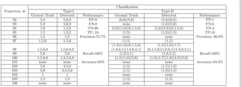
Table 1: Results of classification on Type-I and Type-II anomalies usingλ= 1 andβ = 1.
Classification
Trajectory # Type-I Type-II
Ground Truth Detected Performance Ground Truth Detected Performance
92 5,8 5,6,8 FP:9 (6,8)(5,6) (5,6)(6,8) FP:1
93 5,8 5,6,8 FN:0 none (1,6)(5,6) FN:0
94 1,6 1,5,6 TN:96 (5,6)(1,6)(6,1,5,6) (1,6)(5,6)(6,1,5,6) TN:4
95 1,5 1,3,5 TP: 24 (1,5) (1,3)(1,5) TP:10
96 1,5 1,5 Precision:72.7% none none Precision: 90.9%
97 1,5,6 1,5,6 (1,5) (1,5)
(1,3)(1,6)(6,1,5,6) (1,3)(1,6)(1,7) 98 1,5,6,8 1,5,6,8,9 (1,8,6,1)(1,8,6,5,1) (6,1,5,6)(1,8,6,1)(1,8,6,5,1)
99 5,6 5,6 Recall:100% (1,6,5,1) (1,6,5,1) Recall:100% 100 1,5,6,8 1,3,5,6,8 (1,5)(1,8)(5,6) (1,5)(1,7)(1,8)(4,5)(5,6)
101 none none Accuracy:93% none none Accuracy:93.3%
102 5,6 4,5,6 (1,5) (1,5)(1,6)
103 5,6 3,4,5,6 (1,5) (1,3)(1,5)
104 1 1 none none
105 1,5 1,5 (1,5) (1,5)
Fig. 5: (a) A test trajectory (#94) of the in-house dataset showing Type-I and Type-Type-IType-I anomalous events. (b) RAG representation of the scene and corresponding intra-vertex and inter-vertex movements causing Type-I and Type-II anomalies.
4.2 Results Using Public Dataset
from the RAG that Type-II anomaly with cj = {2,3,4} may appear in the
graph in 32, 72, and 5 ways, respectively. However, no target-trajectory in real-world representing the Type-II anomaly could be found on this dataset.
p(vj|∆) andp(vj|ρi) vales were used to train classifiers associated with
Type-I anomaly. The value of β as mentioned in 16 has been varied between 0.5 and 3.0 during experimentation. The results of classification are presented in Table 2.
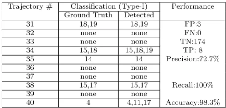
Table 2: Results of classification (Type-I anomaly) of 10 test trajectories of CUHK dataset usingβ = 1.
Trajectory # Classification (Type-I) Performance Ground Truth Detected
31 18,19 18,19 FP:3
32 none none FN:0
33 none none TN:174
34 15,18 15,18,19 TP: 8
35 14 14 Precision:72.7%
36 none none
37 none none
38 15,17 15,17 Recall:100%
39 none none
40 4 4,11,17 Accuracy:98.3%
On the MIT dataset, a subset of 400 trajectories have been used to vali-date the proposed algorithm. Out of the 400, 320 were used to construct the RAG and to estimate the features necessary for training the SVM classifier as depicted in Fig. 4(i). The remaining 80 trajectories have been used for the classification of Type-I anomaly. It is clearly evident from the RAG shown in Fig. 4(i), that Type-I anomaly can possibly appear in 19 different ways. As per the available ground truth, there were 72 instances of Type-I anomalies present in the whole test set covering the 80 test trajectories. The proposed al-gorithm was successful in detecting 109 instances of anomalies assumingβ = 1. When compared against the ground truth, the proposed method recorded false positive, false negative, true positive, and true negative values of 50, 14, 58, and 331, respectively. Precision, recall, and accuracy values were found to be 53.7%, 80.5%, and 85.8%, respectively.
Fig. 6: (a) Frames corresponding to a Type-I anomaly in a test trajectory (#35) of the CUHK dataset. (b) RAG representation of the scene and corre-sponding intra-vertex movements causing the anomaly. (a) Frames correspond-ing to a Type-I anomaly in a test trajectory (#362) of the MIT dataset. (b) RAG representation of the scene and corresponding intra-vertex movements causing the anomaly.
and 14 in MIT dataset); thus making the proposed method quite suitable to support visual analytic solutions in real-time.
4.3 Results Using Custom Dataset
anomalies present in the in-house dataset as per the ground-truth, are 9 and 39, respectively.
In the analysis of Type-I anomaly,p(vj|∆) andp(vj|ρi) are estimated using
the training set and presented to the classifier. Finally, features are computed from the test set and are fed to the classifier. Results of classification are presented in Table 1. For Type-II anomaly, the SVM classifier is trained using
p(Xcj > λ|∆) and p(Xcj > λ|ρi) for cycles of maximum length 5. Further, it has been assumed that 1 ≤ λ ≤ 6 and β is varied between 0.5 and 3.0. The target-trajectories for cj = {2,3,&4} are analysed separately and the
results of classification are summarized in Table 1. Examples of Type-I and Type-II anomalies from a single test trajectory are presented in Fig. 5. It may be observed that the chosen test trajectory has Type-I anomaly within the vertices 1, 5, and 6, whereas, inter-vertex movements between 1-6, 5-6, and 6-1-5-6 are directly related to Type-II anomalies. It can be verified from Table 1, that the proposed method is capable of localizing both types of anomalies with accuracy as high as 93%.
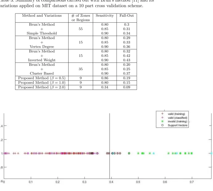
4.4 Comparative Analysis
In this section, a comparative analysis of the proposed approach against the state-of-the-art method of Brun et al. [11] using the various datasets are pre-sented. Since the proposed approach and Brun’s method in [11] differ in their basic methodology and objectives, a direct comparison of results using previ-ously used metrics may not be possible. However, both methods apply scene segmentation and trajectory classification. Therefore, variations in sensitiv-ity and fall-out rate were considered to be good measures for comparison. In Table 3, the summary comparative results using the MIT dataset is presented. Following inferences can be drawn from the results presented in 3. Signif-icantly less false positives have been recorded using the proposed method as compared to the baseline method of [11]. However, as β is increased beyond 1.0, the rate of change of true positives decreases as explained earlier. On the contrary, false positive cases are more in comparison to the different variations of Burn’s method.
4.5 Effect of Key Parameters and Models
In this section, experimental results demonstrating the effect of some of the key parameters and models are reported.
4.5.1 Varying SVM Parameters
Brun’s Method 0.80 0.32
+ 15 0.85 0.42
Inverted Weight 0.90 0.43
Brun’s Method 0.80 0.20
+ 35 0.85 0.25
Cluster Based 0.90 0.37
Proposed Method (β= 0.5) 9 0.86 0.19 Proposed Method (β= 1.0) 9 0.80 0.15 Proposed Method (β= 2.0) 9 0.34 0.09
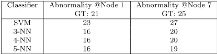
Fig. 7: Demonstration of linearly separable data used in the classification (MIT dataset with respect to region 1).
4.5.2 Effect of Different Classifiers
In addition to experimenting with the SVM classifier, as an alternative mech-anism of classification, the effect of the k-NN based classifier in conjunction with the proposed method has been studied. It can be observed from Table 4 that the k-NN based classifier is not a better choice compared to the SVM counterpart since it fails to detect more true cases. It may also be observed that, the value ofkhas very little effect on the rate of classification.
Table 4: SVM vs kNN Classifiers on MIT dataset (Type-I) analysis withβ= 1.0.
Classifier Abnormality @Node 1 Abnormality @Node 7
GT: 21 GT: 25
SVM 23 27
3-NN 16 20
4-NN 16 20
5-NN 16 19
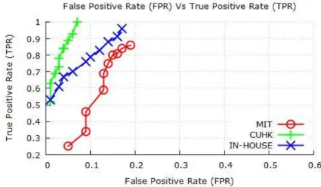
4.5.3 Effect ofβ
The sensitivity of the proposed method can be influenced by the choice of the parameterβ. Therefore, in order to study the effect of the parameterβ on the proposed method,β is chosen to be varied between 0.5 to 3.0 while the true positive and false positive rates are measured. Fig. 8 presents the ROC curves obtained across the different datasets. It can be verified that, high true positive rates are possible in all three cases. However, whenβ is increased beyond 3.0, the rate of increase of false positives, is reduced. This could be because, when
β > 1.0, the classifier is enforced to be biased towards negative samples as given in (16). Therefore, the rate of change of false positives becomes lower in comparison to the rate of change of true positives. On the contrary, when
β is reduced below 1.0, the sensitivity of the proposed method is increased thus classifying a test trajectory as abnormal even under marginal deviation of the trajectory from its average statistics., thus, increasing the number of false positives.
In addition, the effect of β that is used to determine the class of a tra-jectory during preparation of data for training is also presented. It can be observed that, the number of invalid segments at a particular vertex reduces asβ increases. This is in line with the assumption that increasing the value of
Fig. 8: ROC curves obtained by varying β between 0.5 and 2.5.
4.5.4 Computational Complexity
Given that the number of zones or regions can vary in the Brun’s algorithm, the computational overhead is expected to increase as the number of vertices increased. Since the proposed method uses an optimized partitioning of the scene, testing a trajectory against the trained system is computationally ac-ceptable and suitable for online analysis. However, the time required to train the classifiers in the proposed technique is high because of the complex na-ture of the feana-ture extraction process. It has been observed that, the proposed method takes 31 seconds to compute the graph and train the classifiers on the MIT dataset. Testing takes on an average 1-2 seconds, which is often accept-able given that the training can be done offline.
5 Conclusion
Fig. 9: Variation in number of invalid trajectory segments with respect to various nodes/regions of the RAG versesβ value.
The future of this method can have potential applications in analysing crowd behaviour in outdoor as well as indoor environments. Further, a single camera based solution can be designed using the proposed methodology to assist se-curity agencies responsible for maintaining smooth and safe operations inside crowded scene such as in railway stations, airports, busy road junctions, etc. Finally, possible extensions can be made for searching complex anomalies and be combined with target identification.
References
1. D. Gowsikhaa, S. Abirami, R. Baskaran, Automated human behavior anal-ysis from surveillance videos: a survey, Artificial Intelligence Review 42 (4) (2014) 747–765.
6. W. Niu, J. Long, D. Han, Y. Wang, Human activity detection and recog-nition for video surveillance, in: Proceedings of the IEEE International Conference on Multimedia and Expo, Vol. 1, 2004, pp. 719–722.
7. B. Antic, B. Ommer, Video parsing for abnormality detection, in: Pro-ceedings of the IEEE International Conference on Computer Vision, 2011, pp. 2415–2422.
8. R. Hamid, A. Johnson, S. Batta, A. Bobick, C. Isbell, G. Coleman, De-tection and explanation of anomalous activities: representing activities as bags of event n-grams, in: Proceedings of the IEEE Computer Society Conference on Computer Vision and Pattern Recognition, Vol. 1, 2005, pp. 1031–1038.
9. T. Hospedales, J. Li, S. Gong, T. Xiang, Identifying rare and subtle be-haviors: A weakly supervised joint topic model, IEEE Transactions on Pattern Analysis and Machine Intelligence 33 (12) (2011) 2451–2464. 10. M. Krishna, J. Denzler, A combination of generative and discriminative
models for fast unsupervised activity recognition from traffic scene videos, in: Proceedings of the IEEE Winter Conference on Applications of Com-puter Vision, 2014, pp. 640–645.
11. L. Brun, B. Cappellania, A. Saggese, M. Vento, Detection of anomalous driving behaviors by unsupervised learning of graphs, in: Proceedings of the IEEE International Conference on Advanced Video and Signal Based Surveillance, 2014, pp. 405–410.
12. G. Tzanidou, I. Zafar, E. Edirisinghe, Carried object detection in videos using color information, IEEE Transactions on Information Forensics and Security 8 (10) (2013) 1620–1631.
13. K. Lin, S. Chen, C. Chen, D. Lin, Y. Hung, Abandoned object detection via temporal consistency modeling and back-tracing verification for visual surveillance, IEEE Transactions on Information Forensics and Security 10 (7) (2015) 1359–1370.
14. M. Elhamod, M. Levine, Automated real-time detection of potentially suspicious behavior in public transport areas, IEEE Transactions on In-telligent Transportation Systems 14 (2) (2013) 688–699.
15. L. Brun, A. Saggese, M. Vento, Dynamic scene understanding for behav-ior analysis based on string kernels, IEEE Transactions on Circuits and Systems for Video Technology 24 (10) (2014) 1669–1681.
Recognition Workshop, 2008, pp. 1–8.
17. B. Morris, M. Trivedi, A survey of vision-based trajectory learning and analysis for surveillance, IEEE Transactions on Circuits and Systems for Video Technology 18 (8) (2008) 1114–1127.
18. S. Saleh, S. Suandi, H. Ibrahim, Recent survey on crowd density estimation and counting for visual surveillance, Engineering Applications of Artificial Intelligence 41 (2015) 103–114.
19. A. Yilmaz, O. Javed, M. Shah, Object tracking: A survey, ACM Comput-ing Surveys 38 (4) (2006) 1–45.
20. A. Smeulders, D. Chu, R. Cucchiara, S. Calderara, A. Dehghan, M. Shah, Visual tracking: An experimental survey, IEEE Transactions on Pattern Analysis and Machine Intelligence 36 (7) (2014) 1442–1468.
21. J. Batista, P. Peixoto, C. Fernandes, M. Ribeiro, A dual-stage robust vehi-cle detection and tracking for real-time traffic monitoring, in: Proceedings of the Intelligent Transportation Systems Conference, 2006, pp. 528–535. 22. T. Dinh, N. Vo, G. Medioni, Context tracker: Exploring supporters and distracters in unconstrained environments, in: Proceedings of the IEEE Computer Society Conference on Computer Vision and Pattern Recogni-tion, 2011, pp. 1177–1184.
23. Y. Boers, H. Driessen, J. Torstensson, M. Trieb, R. Karlsson, F. Gustafs-son, Track-before-detect algorithm for tracking extended targets, IEE Pro-ceedings on Radar, Sonar and Navigation 153 (4) (2006) 345–351. 24. M. Han, A. Sethi, W. Hua, Y. Gong, A detection-based multiple object
tracking method, in: Proceedings of the IEEE International Conference on Image Processing, Vol. 5, 2004, pp. 3065–3068.
25. H. Veeraraghavan, P. Schrater, N. Papanikolopoulos, Robust target de-tection and tracking through integration of motion, color, and geometry, Computer Vision and Image Understanding 103 (2) (2006) 121–138. 26. S. Oron, Locally orderless tracking, in: Proceedings of the IEEE Computer
Society Conference on Computer Vision and Pattern Recognition, 2012, pp. 1940–1947.
27. Z. Khan, I. Gu, Joint feature correspondences and appearance similar-ity for robust visual object tracking, IEEE Transactions on Information Forensics and Security 5 (3) (2010) 591–606.
28. G. Silveira, E. Malis, Real-time visual tracking under arbitrary illumina-tion changes, in: Proceedings of the IEEE Computer Society Conference on Computer Vision and Pattern Recognition, 2007, pp. 1–6.
29. M. Ekman, Particle filters and data association for multi-target tracking, in: Proceedings of the 11th International Conference on Information Fu-sion, 2008, pp. 1–8.
30. S. Srkk, A. Vehtari, J. Lampinen, Rao-blackwellized particle filter for mul-tiple target tracking, Information Fusion 8 (1) (2007) 2–15.
35. Y. Liu, J. Cui, H. Zhao, H. Zha, Fusion of low-and high-dimensional ap-proaches by trackers sampling for generic human motion tracking, in: Pro-ceedings of the International Conference on Pattern Recognition, 2012, pp. 898–901.
36. V. Mahadevan, W. Li, V. Bhalodia, N. Vasconcelos, Anomaly detection in crowded scenes, in: Proceedings of the IEEE Computer Society Conference on Computer Vision and Pattern Recognition, 2010, pp. 1975–1981. 37. B. Zhao, L. Fei-Fei, E. Xing, Online detection of unusual events in videos
via dynamic sparse coding, in: Proceedings of the IEEE Computer Society Conference on Computer Vision and Pattern Recognition, 2011, pp. 3313– 3320.
38. R. Leyva, V. Sanchez, C. Li, Video anomaly detection based on wake motion descriptors and perspective grids, in: Proceedings of the IEEE International Workshop on Information Forensics and Security, 2014, pp. 209–214.
39. Y. Cong, J. Yuan, Y. Tang, Video anomaly search in crowded scenes via spatio-temporal motion context, IEEE Transactions on Information Foren-sics and Security 8 (10) (2013) 1590–1599.
40. M. Krishna, P. Bodesheim, M. Krner, J. Denzler, Temporal video segmen-tation by event detection: A novelty detection approach, Pattern Recog-nition and Image Analysis 24 (2) (2014) 243–255.
41. F. Nater, H. Grabner, L. Gool, Temporal relations in videos for unsu-pervised activity analysis, in: Proceedings of the British Machine Vision Conference, 2011, pp. 21.1–21.11.
42. D. Kuettel, M. Breitenstein, L. Van Gool, V. Ferrari, What’s going on? discovering spatio-temporal dependencies in dynamic scenes, in: Proceed-ings of the IEEE Computer Society Conference on Computer Vision and Pattern Recognition, 2010, pp. 1951–1958.
43. D. Dogra, R. Reddy, K. Subramanyam, A. Ahmed, H. Bhaskar, Scene rep-resentation and anomalous activity detection using weighted region associ-ation graph, in: Proceedings of the Internassoci-ational Conference on Computer Vision Theory and Applications, 2015, pp. 17–25.
45. B. Zhou, X. Wang, X. Tang, Understanding collective crowd behaviors: Learning a mixture model of dynamic pedestrian-agents, in: Proceedings of the IEEE Computer Society Conference on Computer Vision and Pattern Recognition, 2012, pp. 2871–2878.
46. R. Laxhammar, Chapter 4 - anomaly detection, in: V. N. Balasubrama-nian, S. Ho, V. Vovk (Eds.), Conformal Prediction for Reliable Machine Learning, Morgan Kaufmann, Boston, 2014, pp. 71–97.
47. R. Laxhammar, G. Falkman, Online learning and sequential anomaly de-tection in trajectories, IEEE Transactions on Pattern Analysis and Ma-chine Intelligence 36 (6) (2014) 1158–1173.
48. K. Cheng, Y. Chen, W. Fang, Video anomaly detection and localization using hierarchical feature representation and gaussian process regression, in: Proceedings of the IEEE Computer Society Conference on Computer Vision and Pattern Recognition, 2015, pp. 2909–2917.
49. M. Roshtkhari, M. Levine, Online dominant and anomalous behavior de-tection in videos, in: Proceedings of the IEEE Computer Society Confer-ence on Computer Vision and Pattern Recognition, 2013, pp. 2611–2618. 50. Y. Liu, L. Nie, L. Han, L. Zhang, D. Rosenblum, Action2Activity: recog-nizing complex activities from sensor data, in: Proceedings of the Interna-tional Conference on Artificial Intelligence, 2015, pp. 1617–1623.
51. Y. Liu, L. Nie, L. Liu, D. Rosenblum, From action to activity: Sensor-based activity recognition, Neurocomputing, 181 (2016) 108–115.
52. L. Liu, L. Cheng, Y. Liu, Y. Jia, D. Rosenblum, Recognizing Complex Activities by a Probabilistic Interval-Based Model, in: Proceedings of the AAAI Conference on Artificial Intelligence, Vol. 30, 2016, pp. 1266–1272. 53. Y. Lu, Y. Wei, L. Liu, J. Zhong, L. Sun, Y. Liu, Towards unsupervised physical activity recognition using smartphone accelerometers, Multime-dia Tools and Applications, 76 (8) (2017) 10701–10719.
54. Y. Liu, X. Zhang, J. Cui, C. Wu, H. Aghajan, H. Zha, Visual analysis of child-adult interactive behaviors in video sequences, in: Proceedings of the International Conference on Virtual Systems and Multimedia, 2010, pp. 26–33.
55. V. Saligrama, Z. Chen, Video anomaly detection based on local statistical aggregates, in: Proceedings of the IEEE Computer Society Conference on Computer Vision and Pattern Recognition, 2012, pp. 2112–2119.
56. N. Lia, X. Wua, D. Xud, H. Guoa, W. Fenga, Spatio-temporal context analysis within video volumes for anomalous-event detection and localiza-tion, Elsevier Neurocomputing 155 (1) (2015) 309319.
57. D. Dogra, A. Ahmed, H. Bhaskar, Interest area localization using trajec-tory analysis in surveillance scenes, in: Proceedings of the International Conference on Computer Vision Theory and Applications, 2015, pp. 31– 38.
IEEE Transactions on Information Forensics and Security 8 (10) (2013) 1610–1619.
62. N. Alon, R. Yuster, U. Zwick, Finding and counting given length cycles, Algorithmica 17 (1997) 209–223.
63. J. Flum, M. Grohe, The parameterized complexity of counting problems, SIAM Journal on Computing 33 (4) (2004) 892–922.
64. Y. Liu, Y. Liang, S. Liu, D. Rosenblum, Y. Zheng, Predicting urban water quality with ubiquitous data, in: arXiv preprint, 2016, 1610.09462. 65. Y. Liu, Y. Zheng, Y. Liang, S. Liu, D. Rosenblum, Urban water quality
prediction based on multi-task multi-view learning, 2016.
66. Y. Liu, L. Zhang, L. Nie, Y. Yan, D. Rosenblum, Fortune Teller: Predicting Your Career Path, in: Proceedings of the AAAI Conference on Artificial Intelligence, 2016, pp. 201–207.
67. D. Preotiuc-Pietro, Y. Liu, D. Hopkins, L. Ungar, Beyond binary labels: political ideology prediction of Twitter users, in: Annual meeting of the association for computational linguistics, 2017.
68. S. Abe, Support vector machines for pattern classification, Vol. 53, Springer-Verlag, 2005.