Theses
8-2018
Novel Detection and Analysis using Deep
Variational Autoencoders
Tucker B. Graydon
Follow this and additional works at:https://scholarworks.rit.edu/theses
This Thesis is brought to you for free and open access by RIT Scholar Works. It has been accepted for inclusion in Theses by an authorized administrator of RIT Scholar Works. For more information, please [email protected].
Recommended Citation
Deep Variational Autoencoders
by
Tucker B. Graydon
A Thesis Submitted in Partial Fulfillment of the Requirements for the Degree of Master of Science in Electrical and Microelectronic Engineering
Supervised by
Professor Dr. Ferat Sahin
Department of Electrical and Microelectronic Engineering Kate Gleason College of Engineering
Rochester Institute of Technology Rochester, New York
August 2018
Approved by:
Dr. Ferat Sahin, Professor
Thesis Advisor, Department of Electrical and Microelectronic Engineering
Dr. Sohail Dianat, Professor
Committee Member, Department of Electrical and Microelectronic Engineering
Dr. Ahmet Okutan, Professor
Rochester Institute of Technology Kate Gleason College of Engineering
Title:
Novel Detection and Analysis using Deep Variational Autoencoders
I, Tucker B. Graydon, hereby grant permission to the Wallace Memorial Library to
reproduce my thesis in whole or part.
Tucker B. Graydon
Acknowledgments
Throughout my undergraduate and graduate studies here at RIT, there are many who
deserve my gratitude.
Foremost, I must thank Dr. Ferat Sahin. You have been a constant source of advice and
wisdom for me and it is through your guidance and encouragement
that I am here today.
Shitij, you have been there at all hours of the day and night supporting me and engaging in
long conversations that pushed my work further ahead. You are truly a good mentor and
good friend.
Ryan, I have known you in many capacities over the years. In them all, you always
provided me with invaluable perspective and counsel, which has made me a better
engineer. This work would not have been possible without your influence.
Celal, you have always been the never-ending optimist in our lab, keeping us going even
at 2am the day before finals.
Last, I would like to say thank you to Sadie, your support through countless long nights
and difficult semesters made it all worth it.
Abstract
Novel Detection and Analysis using Deep Variational Autoencoders
Tucker B. Graydon
Supervising Professor: Dr. Ferat Sahin
This paper presents a Novel Identification System which uses generative modeling
tech-niques and Gaussian Mixture Models (GMMs) to identify the main process variables
in-volved in a novel event from multivariate data. Features are generated and subsequently
dimensionally reduced by using a Variational Autoencoder (VAE) supplemented by a
de-noising criterion and a βdisentangling method. The GMM parameters are learned using
the Expectation Maximization(EM) algorithm on features collected from only normal
op-erating conditions. A one-class classification is achieved by thresholding the likelihoods
by a statistically derived value. The Novel Identification method is verified as a detection
method on existing Radio Frequency (RF) Generators and standard classification datasets.
The RF dataset contains 2 different models of generators with almost 100 unique units
tested. Novel Detection on these generators achieved an average testing true positive rate
of 97.31% with an overall target class accuracy of 98.16%. A second application has the
network evaluate process variables of the RF generators when a novel event is detected.
This is achieved by using the VAE decoding layers to map the GMM parameters back to
a space equivalent to the original input, resulting in a way to directly estimate the process
List of Contributions
• T. Graydon, F. Sahin, “Novel Detection and Analysis usingβ-DVAE Networks,”
Sys-tems, Man and Cybernetics (SMC), 2018 IEEE International Conference, 2018.
. . . iii
Acknowledgments . . . iv
Abstract. . . v
List of Contributions. . . vi
1 Introduction . . . 1
2 Background Literature . . . 3
2.1 One-Class Classification . . . 3
2.2 Mixture Models . . . 4
2.2.1 Gaussian Mixture Models . . . 6
2.3 Generative Modeling . . . 7
2.4 Autoencoders . . . 9
2.5 Denoising Criterion . . . 11
2.6 Variational Autoencoders . . . 15
2.6.1 Variational Bayes . . . 15
2.6.2 Autoencoded Variational Bayes . . . 19
2.7 β- Disentangled Representation . . . 20
3 Proposed Method . . . 23
3.1 Dataset . . . 24
3.2 Preprocessing . . . 26
3.3 β-DVAE Network . . . 27
3.4 GMM Classification . . . 30
3.5 Classifier Estimation inn-Dimensions . . . 31
4 Results . . . 34
4.1 Latent Model Results . . . 34
4.2 Decoded Model Results . . . 40
5 Conclusions . . . 44
6 Future Work . . . 46
2.1 The selection ofk centroids is key for fitting the data. A lowkmay cause an over-generalized model and a high value will lead to overfitting. . . 6 2.2 A Standard Autoencoder Layout . . . 10 2.3 The denoising criterion modifies a typical autoencoder by adding a
stochas-tic mapping layer to locally corrupt an input. . . 12 2.4 Corruption from a Manifold perspective. Assume dataxis concentrated on
a low dimension manifold. Corrupted examples are created by applying a corrupting processC( ˜x|x), these will lie further from the manifold. g(f( ˜x)) is then used to project them back onto the manifold [1]. . . 13 2.5 Kingma and Wellings’ autoencoding variational Bayes method with the
reconstruction term for backpropagation. . . 18
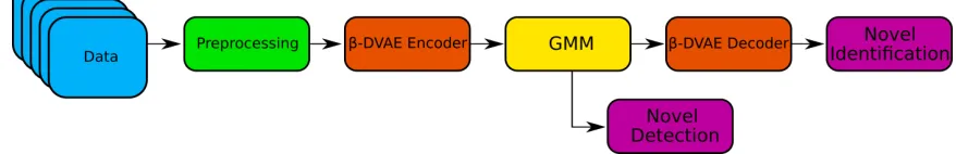
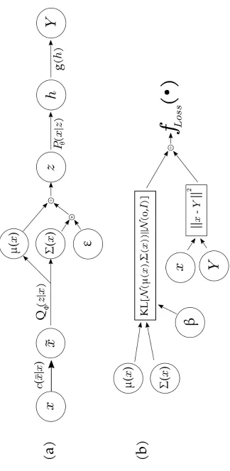
3.1 The System Overview for Novel Detection and Identification . . . 23 3.2 Data Samples from the MNIST Dataset. . . 24 3.3 Proposed Method Process flow. The forward pass (a) and the loss
calcula-tion (b). . . 29
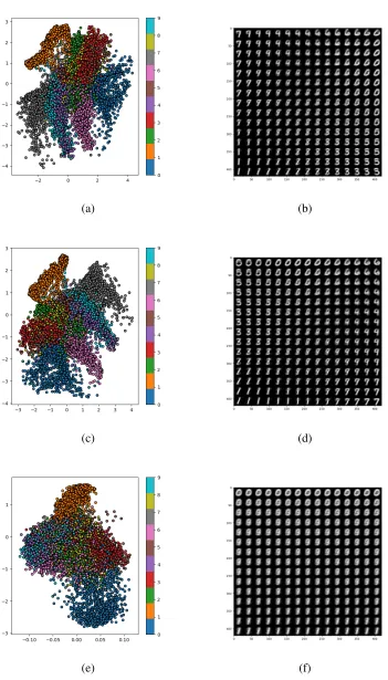
4.1 Latent 2D mapping of MNIST digits with reconstructed digits sampled from the latent space. (a)(b)β=1, (c)(d)β =2, (e)(f)β= 7 . . . 36 4.2 A 2D embedded view of MKS generator normal operation samples (green)
and seeded faults (purple). . . 37 4.3 Network Loss during training over 1000 epochs. Mean squared error was
used for the reconstruction loss and aβweighted KL divergence was added to the MSE loss. . . 38 4.4 Performance Metrics accuracy and true positive rate of the GMM
classifi-cation with PCA as the feature extractor. Results are reported as the mean of 10 trials while varying the number of PCA components used for features. 39 4.5 Performance Metrics accuracy and true positive rate of the GMM
classifi-cation withβ-DVAE Encoder network as the feature extractor. Results are reported as mean of 10 trials while varying the size of the encoded feature vectors. . . 39
4.6 Per-variable likelihood analysis by theβ-DVAE-Decoded model (k=3) of three types ofnon-normal generator data. The log-likelihoods have been normalized by the threshold value indicated in order to emphasize variables that arenon-normal. . . 40 4.7 Per-variable likelihood analysis by theβ-DVAE-Decoded model (k=8) of
three types ofnon-normal generator data. The log-likelihoods have been normalized by the threshold value indicated in order to emphasize variables that arenon-normal. . . 41 4.8 Decoded GMM model performance over varying sizes of the latent feature
3.1 Dataset names, sample counts, and class descriptions. . . 25
4.1 One-Class Classification comparison of True Positive Rate ofnormalclass. 37
4.2 β-DVAE-GMM comparison with state-of-the-art classification methods [2].
Results are reported as mean per-class accuracy of 10 trials with standard
deviation in parenthesis. . . 38
4.3 Number of mixtures, Accuracy, True Positive Rate and Specificity of
Trans-formed GMMs. Results are reported as mean of 10 trials with standard
deviation in parenthesis. . . 38
4.4 MKS Generator System Variables, Environmental Variables, and Lifetime
indicators for fault analysis. . . 42
Chapter 1
Introduction
Current systems in the Integrated Circuit (IC) manufacturing and fabrication industry
de-pend on the reliability and availability of the process equipment. Any failures of process
machinery mean down time, ruined products, resources lost, and an overall increase in the
cost of ownership for the company. Tools such as RF plasma generators are critical in the
IC fabrication process. In order to maximize production and minimize cost of ownership,
the reliability and operation of these components is critical. There are currently tools
avail-able to monitor system health, however the ability to analyze the symptoms of the failure
can dramatically shorten machine down time, keeping cost of ownership low.
Novel event detection, specifically fault detection and identification are a derivative of
statistical process control. In recent years it has been shown that the addition of machine
learning leads to better fault detection [3]. Current fault detection methods are based on
modeling a system and detecting deviations from a model of a normalsystem. Previous
work has been done with regard to modeling systems and classifying operations as
nor-malornot-normal. Gaussian Mixture Models [4] [2] [5], Support Vector Machines (SVM)
[6], Radial Basis Function Networks (RBFN) [7][8], Deep Autoencoders [9] and Novelty
modified Novelty Detection Framework (NDF) has been an inspiration for the work
pre-sented in this paper. The results of the NDF as well as Bowen’s embedded application
validate the additional need for an initial report analyzing the fault event at the input level.
This novelty analysis methodology will attempt to utilize previous one-class
classifica-tion methods along with generative neural network architectures in order to detect a novel
event as well as relate the learned one-class classifier parameters back to the original
pro-cess variables. By relating the classification model back to the input space the fitness of
each process variable can be estimated and can be used to reduce the down time of the
system.
This paper outlines the use ofβ-Disentangling, Denoising Variational Autoencoders (β
-DVAE) with a GMM one-class classifier as a fault detection and analysis system for RF
plasma generators. The remainder of this paper will follow this outline: Section II defines
β-DVAE and GMM, Section III explains the proposed method in detail, and Section IV
Chapter 2
Background Literature
One-Class Classification
The basis of machine learning is that a set of data which represents some parameters or
features of a system where all possible inputs and outputs are uniformly represented. This
is labeled as the training set of data. In the field of fault analysis and detection there is
no practical way of obtaining faulty data from all possible modes of fault or failure. It is
more common that there exists significant data of the desired mode of operation. Typically,
fault analysis methods utilize multi-class classifiers, in these multi-class situations machine
learning methods such as support vector machines, neural networks, radial basis functions
and Bayesian networks are used. Typical machine learning methods rely on the availability
of data for training the models. Therefore, the machine learning methods can only be as
successful as the data available during training. For multi-class methods both the target and
non-target class data must be available. There is a common difficulty in collecting data from
non-target classes, specifically non-normal operation modes. Since there is an immense
difficulty associated with collecting reliable data fromevery possible mode of failurethere
has been a paradigm shift towards learning only the normal modes of operation for a system
The assumption of one-class classification is that information is only available from one
class, the target class. The problem one-class classification poses is defining a boundary
around the target class in order to maximize target acceptance and minimize non-target
acceptance. The two most popular one-class realizations are density based and boundary
based approaches. Density based methods estimate the densities of the training data and
determine threshold values. Estimating the densities can be accomplished using many
dif-ferent distributions such as Gaussian, Poisson, Bernoulli and mixtures of these. Density
based methods can be very effective as long as there is sufficiently large training data and a
proper model is applied. In the case of limited training samples, density based methods will
not generalize the data appropriately. It is therefore appropriate to solve the problem with
the available data and use boundary methods to separate the target data. The commonly
used boundary based methods include k-means, k nearest neighbor (KNN), and support
vector data description (SVDD). These boundary based methods are capable of working on
small dataset sizes but are heavily reliant on distance measures and very sensitive to feature
scaling.
Mixture Models
Mixtures of distributions are commonly used as mathematical methods for statistical
mod-eling of a set of data. Mixture models have been applied as clustering and latent class
analysis and are generally favored for their ability to provide descriptive models for a data
dimensional data can be represented as a finite number of K components, with some
un-known proportions.
The general formulation of a mixture model is as follows: An observed random
vari-able is denoted asy1, ...,yN such thatyj is a random vector with probability density
func-tion f(yj) ∈ RM and j = 1, ...,N. Therefore yj contains M measurements of the jth
ob-served sample of random variables and Y = (yT1, ...yTN)T contains all observed samples.
The probability density function of an observed random variable, in parametric form for a
K-component mixture is:
f(yj;Ψ)= K
X
i=1
πifi(yj;θi) (2.1)
TheΨterm here represents any unknown parameters of the mixture model and can be
expressed below, where aξterm is used to represent alla prioriparameters inθ.
Ψ =(π1, ..., πK, ξT)T (2.2)
Lettingπ =(π1, ..., πT)T be a vector of mixing weights wherePKi=1πi = 1. Equation 2.1
is the general form of a mixture model. For the complete realization, a distribution must be
Gaussian Mixture Models
The Gaussian Mixture model is a mixture model that assumes data is approximately
[image:18.612.146.487.198.410.2]Gaus-sian distributed.
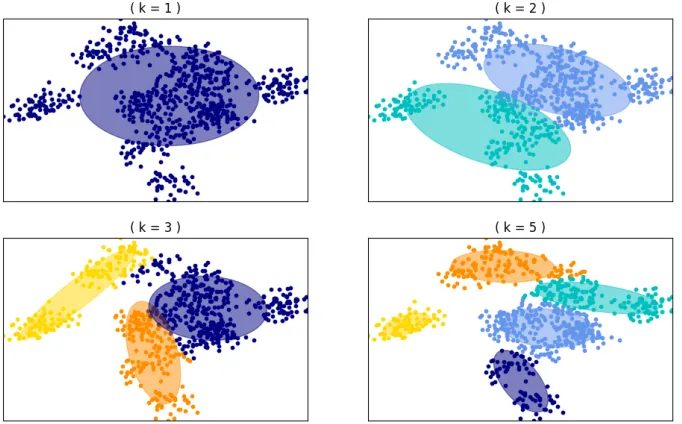
Figure 2.1: The selection ofk centroids is key for fitting the data. A lowk may cause an over-generalized model and a high value will lead to overfitting.
A Gaussian Mixture Model is defined as a combination ofkcombinations of Gaussian
densities. A Gaussian density in d-dimensional space is characterized by a meanµ ∈ Rd
and ad×dcovariance matrixΣ[10][11]. The Gaussian density function is then defined as:
g(x|µ,Σ)=(2π)−d/2|Σ|−1/2exp− 1
2(x−µ) TΣ−1(
Akcomponent Gaussian mixture is defined by:
p(x)= k
X
i=1
πig(x|µi,Σi) (2.4)
Whereπi are weight values for each mixture andg(x|µi,Σi) is the ith mixture density.
The weighted densities are summed into a Gaussian mixture model. The target class and
outliers can then be identified by thresholding the calculated Gaussian likelihoods whereµ
andσare the mean and standard deviation of the training data’s log-likelihood values.
Lth =µL−λ
√
σL (2.5)
There are two popular methods for learning the parameters of the mixture models,
Ex-pectation Maximization (EM) and Variational Bayesian Inference. The EM algorithm is an
iterative process used to calculate the maximum likelihood estimation (MLE) with
miss-ing or unknown data. An iteration of EM is comprised of two steps, an expectation step
followed by a maximization step. In the expectation step, the unknown or missing data is
estimated with respect to the observed data and the current estimates of the model
parame-ters. Then the maximization step maximizes the likelihood of the data with the assumption
that the missing data is known. This process iterates until the model parameters converge.
Generative Modeling
The goals of generative modeling are two-fold: (1) Learn a latent representation of a
a model to generate accurate samples from the latent variables. When applied with
one-class one-classification the generative model encodes the data to latent representations for easier
classification [12] and can scale a model learned in the latent space to the input space. The
remainder of this section defines variational autoencoders, the denoising criterion, β-VAE
and GMMs for one-class classification.
The traditional autoencoder architecture has been utilized since the 1980’s as a method
for linear and non-linear dimension reduction. The fundamental principle of the
autoen-coder is the bottleneck design where an input is mapped down to a lower dimension and
then remapped to reconstruct the ordinal data. This mapped latent variable set is
com-monly used for training machine learning models in a less computationally intensive space.
However, the networks’s ability to apply non-linear mappings is limited to the non-linear
activation functions applied in the hidden layers. Utilizing activations such as sigmoidor
tanh allow for non-linearities in the mapping but significantly increase the risks of
dimin-ishing gradients in larger networks.
There have been attempts to increase the flexibility and strength of the autoencoders
latent variable mappings. Denoising criteria, sparsity and contractive penalties, as well as
stochastic parameterizations of layer weights have been applied to create more salient and
unique latent variables. This push for better encoding of high dimension data has also been
spurred on by growing interest in the field of generative models and deep learning. These
new methodologies learn to map the inputs to latent dimensions and then attempt to sample
Autoencoders
Some of the generative modeling architectures discussed above exploit a particular type of
neural network, an auto-associator, this is also called an autoencoder or a Diabolo network.
There are also connections between the autoencoder and Restricted Bolzman Machines
(RBM). Because of the simplicity of training a shallow autoencoder network they have long
been used to initialize larger networks or to aid in the training of much deeper networks
where each layer has an associated autoencoder that can be trained separately.
An autoencoder is trained to encode an input in some representation such that the input
can be reconstructed from that representation. Therefore the target is the input itself. If a
single hidden linear layer and a mean squared error is used as a criterion for training the
network, the k hidden units learn a projection of the data into thek principal components
of the data. This architecture converges to match principal component analysis (PCA)
pro-jections. Changing the hidden layer to a non-linear function causes the network to behave
very differently from standard PCA and kernel PCA with a linear kernel. This
non-linearity allows the network to capture multi-modal aspects of the input distribution. The
most common generalization of this design switches the mean squared error for minimizing
a negative log-likelihood of reconstructing the input:
LRE =−logP(x|c(x)) (2.6)
distributed representation that captures the main factors of variation in the data.
Figure 2.2: A Standard Autoencoder Layout
There is a large risk in the design of these networks. Given there are no other
con-straints on the system, ann-dimensional input and a hidden layer with a size greater thann
has the potential to learn the input exactly, learning the identity function for the mapping.
It has been disputed introducing constraints such as early stopping and L2 regularization
with stochastic gradient descent can allow an over-complete hidden layer to learn useful
representations, however this still introduces more constraints than just an over-complete
layer and is beyond the scope of this research. Instead, or in addition to adding
regular-ization to the network, one strategy is to incite marginal noise in the encodings which will
be discussed in later sections. Other methods used to force the autoencoder to learn useful
representations include imposing a sparsity constraint on the reconstruction/loss criterion,
Denoising Criterion
One of the central objectives of machine learning is the ability to generalize new
config-urations of observable variables from training data. In the most general sense this means
determining how to redistribute the probability density associated with each training
exam-ple from the empirical distribution. One approach to achieving this goal is through manifold
learning which is attempting to model an embedded lower dimensional manifold that the
high dimension data originates from. Parzan density estimation and principal component
analysis (PCA) have been used for this in the past, however they suffer from isotropic
vari-ances or are limited to only linear manifolds. In a majority of manifold learning methods,
the local shapes for the manifold are defined by a basis indicating the plausible directions
of variation, i.e. a tangent plane to the point on the manifold. Most methods then diverge
on how to combine these local tangential planes along the manifold in order to model the
global manifold structure or density. The focus on local generalizations for these methods
leads to issues with erratic manifolds that have many peaks and valleys. This correlates
with the curse of dimensionality where, in order to learn the global manifold, the required
training examples increases exponentially with manifold complexity. Recently non-linear,
non-locally generalizing manifold learning methods have been produced using deep
learn-ing methods such as autoencoders. Denoislearn-ing and contractive autoencoders (DAE, CAE)
have great promise as manifold learning methods that can achieve local generalization
with-out being restricted to local learning.
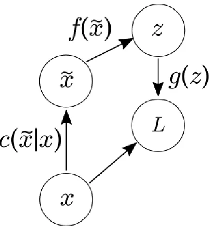
Figure 2.3: The denoising criterion modifies a typical autoencoder by adding a stochastic mapping layer to locally corrupt an input.
by either physically varying the training data locally with corruption, or by adding a
pe-nalizing term targeting local variances. The contractive autoencoder modifies the objective
function of traditional autoencoders by adding the Frobenius norm of the Jacobian of the
input and the latent encoding. This regularizing term penalizes the sensitivity of the input
features to local variances. The denoising approach corrupts an input random variable (x)
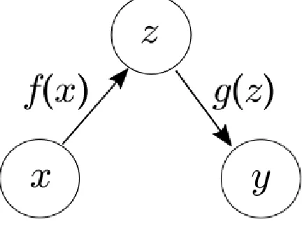
using a known conditional distributionC( ˜x|x). The DAE is trained to estimate the reverse
conditionalg(f( ˜x)) orP(x|x˜) in order to determine a consistent estimator ofP(X).
The typical autoencoder structure takes an inputx ∈ [−1,1]d, and maps it to a hidden,
latent representationz∈[−1,1]d0 by a deterministic mappingz= f
θ(x)= Wx+b,
parame-terized byθ= {W,b}. HereWis ad0×dweight matrix andbis a bias vector. Thezlatent
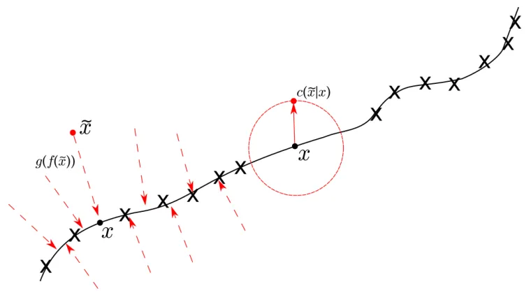
Figure 2.4: Corruption from a Manifold perspective. Assume data x is concentrated on a low dimension manifold. Corrupted examples are created by applying a corrupting processC( ˜x|x), these will lie further from the manifold.g(f( ˜x)) is then used to project them back onto the manifold [1].
mapping is defined byy = gθ0(z) = W0z+b0, withθ0 = {W0,b0}. The weight matrix W0
of the reverse mapping can have additional constraints imposed such as W0 = W, which
is termed tied-weights. Using this method each input variable x is mapped to to a latent
variable inzwhich is then reconstructed toy. The parameters of this model are optimized
to minimize the average reconstruction error between xandyas shown in Eq. 2.7.
θ∗, θ0∗=
arg min θ∗,θ0∗
1
n
n
X
i=1
L
xi,zi
= arg min θ∗,θ0∗
1
n
n
X
i=1
L
xi,gθ0 fθ(xi)
(2.7)
HereLis any loss function such as squared errorL(x,y)=kx−yk2or if the data can be
considered analogous to bit vectors or probabilities, the cross-entropy loss (Eq. 2.8) may
LH(x,y)=− d
X
k=1
xklogyk +(1−xk) log(1−yk)
(2.8)
The denoising criterion modifies the original autoencoder by corrupting the input data
point and training the network to predict/reconstruct the original, uncorrupted input. The
corruption process, defined asC( ˜x|x) represents the conditional distribution over the
cor-rupted samples ( ˜x), given the original input x. By training an autoencoder with this new
input the network is learning the reconstruction distribution,Preconstruct(x|x˜).
In traditional autoencoders the addition of corruption to the input layer is commonly
used to increase the encoding and decoding network’s resilience to noise in the input data.
VAEs with the denoising criterion can be trained similarly to the way denoising
autoen-coders are trained:
1. Sample an input with injected noise ˜x∼ p( ˜x|x)
2. Samplez∼q(z|x˜) and
3. Sample the reconstructed data from the decoder network pθ(x|z) [13][14].
Since the inference network has been modified by the injected noise the objective function
is modified from the traditional VAE:
Variational Autoencoders
Autoencoding variational Bayes was proposed by Kingma and Welling as an approach to
efficiently estimate the posterior inference. The aim of this method of inference is to
ap-proximate a joint distributionQ(x;θ) over a latent variable space xin order to approximate
the true joint distributionP(x) using the Kullback-Liebler Divergence to define “closeness”.
When this method of inference is utilized with the architecture of neural networks, the
sim-ilarity to traditional autoencoders is the rough bottleneck design and the target class being
the input itself. The similarities to autoencoders end there. The loss function used by a
VAE includes the typical reconstruction loss such as mean squared error or smooth L1 loss
as well as a divergence term for the approximate posterior being estimated.
Variational Bayes
A core problem in modern statistics is the approximation of complex probability densities.
Bayesian statistics frame inferences as a calculation of the posterior. From the perspective
of the core problem, this leads to Bayesian models that have difficult posteriors which need
to be approximated.
One popular method of approximating the posterior is known as Markov Chain Monte
Carlo (MCMC) Sampling. This method relies on repeat sampling given the prior and a
likelihood function. Since this method inherently relies on the volume of samples for
ac-curacy, the accuracy of the estimated posterior increases the longer the methods runs. A
given real world resource restrictions.
This is where Variational Inference methods can be a more viable option. Variational
Inference is a machine learning approach to solving these probability density
approxima-tions. When comparing Variational Inferencing (VI) to MCMC methods, it is noted that VI
is faster and better at scaling with larger data than MCMC.
Variational Inference aims to use a latent variable space for optimizing conditional
den-sities given a prior. Variational inference turns the approximation problem into an
opti-mization problem by optimizing the fit of “variational parameters” in the latent distribution
such that the KL divergence is minimized for the density of interest. The conditional
den-sity given an observed input variable xand the latent variablezis as follows:
p(z|x)= p(z,x)
p(x) (2.10)
p(x)=
Z
p(z,x)dz (2.11)
In order to calculate the p(x) term, known as the evidence, the latent variables are
reduced from the joint density shown in Eq. 2.11. This integral term is not always available
in a closed form or is an exponential amount of time necessary to solve it. VI does not
aim to solve this intractable solution but to find a lower bound to the term and optimize
around the lower bound. A family of densitiesDis specified over the latent variables with
each q(z) ∈ D being a candidate for approximating the conditional. The optimization is
solving an optimization problem rather than an intractable integral.
q∗(z)=argminq(z)∈DKL(q(z)kp(z|x)) (2.12)
Hereq∗(·) is the optimum approximation of the conditional given the family of densities
D. This solution still has a dependence on logp(x) from the KL divergence calculation, as
shown below.
KL(q(z)kp(z|x))=E[logq(z)]−E[logp(z|x)] (2.13)
KL(q(z)kp(z|x))=E[logq(z)]−E[logp(z,x)]+logp(x) (2.14)
Decomposing the KL divergence reveals an existing dependency on the evidence. Since
this calculation is still intractable, optimization over a different objective that is equivalent
to the KL divergence is performed. Declaring the logp(x) equivalent to a constant in Eq.
2.14 the negative KL divergence can be used as a lower bound of the evidence, this is
dubbed the Evidence Lower Bound (ELBO).
ELBO(q)= E[logp(z,x)]−E[logq(z)] (2.15)
ELBO(q)=E[logp(x|z)]−KL(q(z)kp(z)) (2.16)
log likelihood and the KL divergence between the p(z) prior and theq(z) candidate.
Dis-secting the ELBO terms reveals how VI can optimize the placement of zvalues over this
objective. The first term is the log likelihood of q(z) mapping values to configurations
in the latent variables that explain the observable data. The second term is the negative
KL divergence of the candidate and the prior, this promotes densities that are similar to the
[image:30.612.136.489.278.433.2]prior. In this way, the objective is attempting to find a balance between likelihood and prior.
Figure 2.5: Kingma and Wellings’ autoencoding variational Bayes method with the reconstruction term for backpropagation.
It is also a interesting that the first term in the ELBO equation 2.16 is the expected
complete log likelihood which can be optimized by the Expectation Maximization (EM)
algorithm. EM uses the fact the ELBO equation is the log likelihood ( logp(x) ) when the
candidate is the joint conditional, q(z) = p(z|x). EM will be discussed in further detail in
later sections. While EM assumes theE[logp(z,x)] is tractable, a variational Bayes EM is
possible where the expectation calculation is replaced with a lower bound on the marginal
Autoencoded Variational Bayes
Kingma and Welling introduced a practical estimator for the lower bound and its derivatives
utilizing the neural network architecture of autoencoders. A approximate posterior in the
form ofqφ(z|x) is assumed, thoughqφ(z) can also be used if the estimator is not conditioned
over x. Under certain conditions, for a chosen approximate posteriorqφ(z|x), the random
variablezcan be re-parameterized using the differential transformationgφ(,x) of auxiliary
noise ∼N(0,I) :
˜
z=gφ(,x) with ∼ p() (2.17)
The appropriate selection of a distribution for p() and function qφ(,x) will be
dis-cussed in a later section. For now, form Monte Carlo estimates of expectations of some
function f(z) w.r.t.qφ(z|x):
Eqφ(z|xi)[f(z)]=Ep()
f(gφ(,xi))
' 1
L
L
X
l=1
f(gφ(l,xi)) where l ∼ p() (2.18)
Applying this technique to the variational lower bound (Eq. 2.16) yields Kingma and
Welling’s Stochastic Gradient Variational Bayes (SGVB) estimator.
Given an observation x, the inferred posterior distribution of the latent variable z is
described by qφ(z|x). The prior p(z) is then assumed to be a isotropic unit Gaussian
model is then defined by a parametric distribution pθ(x|z). This system is modeled
us-ing an autoencoder structure with the encoder/inference network learning φ and the
de-coder/generativenetwork learningθ.
The objective of the VAE is to maximize the marginal likelihood of the observed xin
expectation over the whole distribution ofz.
Dvae(θ, φ,x)= KL(qφ(z|x)||pθ(z)) (2.19)
˜
Lvae(θ, φ,x)=Eqφ(z|x)(logpθ(x|zi))− Dvae (2.20)
The first term in Eq. 2.20 is the reconstruction accuracy of the network’s output to
the original input. The second term is the Kullback-Leibler divergence (KL), from Eq.
2.19, of the posterior to the prior, which acts as a regularizer. However, in order for
back-propagation to be used on the variational parametersφ,zneeds to be re-parameterized as a
function of i.i.d noise () and the output of the encoder network[15] shown in Eq. 2.21.
z=gφ(,x) (2.21)
∼ N(0,I) (2.22)
β
- Disentangled Representation
Research into disentanglement has become increasingly popular with the introduction of
The definition of disentanglement is closely related to the development of these methods,
it is the process by which key aspects of the input data are encoded into specific latent
dimensions. A simple example can be given where an input dataset consists of colorful
geometric shapes of multiple sizes. A perfectly disentangled latent variable space would
have a latent variable representing the color of the object, another variable would encode
the shape present and another may map to the size of the shapes. By having a perfectly
dis-entangled representation such as this, any possible color, shape and size combination could
be generated with just these three latent variables. This aspect of reducing and isolating
features to easily controlled variables drives current improvements in generative modeling.
The stronger the encoded features are the more likely a meaningful sample can be
gener-ated from the network.
β-VAE is a modified VAE method for learning disentangled latent representations of
data in an unsupervised manner [16]. The method introduces a hyperparameter β which
weights the KL divergence term of the standard VAE (β = 1) objective as defined in Eq.
2.23. A disentangled representation is defined as one where single latent units are sensitive
to changes in single generative factors, while being invariant to changes in others [17]. An
example being a 3D object dataset where the learned disentangled latent variables encode
the scale, orientation, color and object identity.
Dβ−vae(θ, φ, β,x)= β·KL(qφ(z|x)||pθ(z)) (2.23)
pressure to learn the disentangled representations [16]. Aβ-VAE withβ = 1 is equivalent
to the original VAE equation by Kingma and Welling [15]. Therefore, a β > 1 is key for
applying pressure on the network during training. There is a trade-offbetween
reconstruc-tion accuracy and the quality of the representareconstruc-tions inzwith higherβvalues and soβmust
Chapter 3
Proposed Method
This chapter outlines the proposed method of detecting and analyzing novel events using a
β-VAE network with a GMM classifier. The chapter is organized as follows: first the data
set collection method and organization are discussed, and the preprocessing methods used.
The design of theβ-VAE network is outlined and the GMM classifier is outlined as well.
This classifier is composed of two parts, the latent classifier model and the projection of the
model parameters to a different feature space for process variable processing. Finally, the
model parameter mappings are outlined with the use of Lediot-Wolf covariance estimation
[image:35.612.88.527.605.676.2]in order to represent the GMM in the process variable space.
Dataset
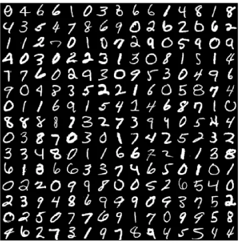
Figure 3.2: Data Samples from the MNIST Dataset.
In order to demonstrate the β-VAE network can operate as a standard classification
method, as well as novel analysis, standard datasets were utilized to compare the β-VAE
method to state-of-the-art classifiers. The two most common multivariate two-class datasets
were selected from the UCI Machine Learning Repository [18], multi-class datasets can be
used as well with one class being chosen as the target one-class. The cancer evaluation
dataset, as well as the ionosphere testing datasets were chosen to compare classification
performance. The MNIST handwriting dataset was also used as validation theβ-VAE
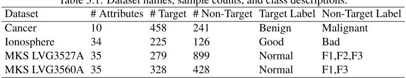
Table 3.1: Dataset names, sample counts, and class descriptions.
Dataset # Attributes # Target # Non-Target Target Label Non-Target Label Cancer 10 458 241 Benign Malignant Ionosphere 34 225 126 Good Bad MKS LVG3527A 35 279 899 Normal F1,F2,F3 MKS LVG3560A 35 328 428 Normal F1,F3
attributes, sample counts and target class for each dataset. In order to adhere to one-class
classification techniques the target class chosen was the class most likely to represent
nor-malconditions. For the cancer dataset the benign class was considered the target class and
for the ionosphere data the “good” class was the target class. The state-of-the-art classifiers
used for comparison were: k-Nearest Neighbor (k-NN) [20], Support Vector Machine with
a radial basis kernel function (SVM-RBF) with Principal Component Analysis (PCA), and
GMM with PCA [2]. These methods were chosen in order to compare simple methods
such ask-NN, as well as methods similar to the proposed approach, such as SVM-RBF and
GMM with PCA.
The primary dataset that was focused on in the experimental results was operational
data collected from the MKS LVG3527A 27MHz RF generator and the MKS LVG3560A
60MHz generator [4][2]. Multivariate, time-series data, or fingerprints, were collected and
provided by MKS ENI Products. These fingerprints were collected from generators during
normal operating conditions during three different load conditions. The load conditions
wereFifty Ohms, ShortandOpen. These conditions simulate full operational loads of the
RF generators. Along with the knownnormaloperational data, additional fingerprints were
collected while generators were operating with 3 seeded faulty conditions; which are listed
1. Faulty Amplifier
2. Poor Solder Joints on Resistors
3. Poor Solder Joints on FETs
Thesenon-normalconditions were chosen to closely mimic scenarios where the current
quality control measures experience difficulty identifyingnon-normaloperations. In order
to evaluate the data, the fingerprints of each generator were partitioned into training,
vali-dation and testing. Thenormalfingerprints were split into 60% training and 20% validation
and 20% testing while thenon-normal fingerprints were separated 40/60% for validation
and testing respectively.
Preprocessing
Before the data could go through the β-VAE network it needed to be processed in order to
learn faster and more accurately. First the training data is rescaled to a maximum of+1 and
a minimum of−1.
Xscaled= −2·
X−min(X)
max(X)−min(X) +1 (3.1)
Then each variable has its mean subtracted in order to zero-mean the signals. All
validation and testing data for consistency.
β
-DVAE Network
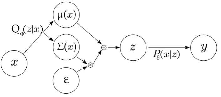
Theβ-DVAE model is designed with traditional VAE architecture in mind. It is comprised
of a stochastic encoding network and a decoding network which maps inputs into a
sub-space z. The encoder has an initial denoising layer, this has intentionally been designed
to be overcomplete since this has shown to produce better manifold learning. The level of
noise injected can be controlled by a hyper parameter which modifies the magnitude and
standard deviation of the Gaussian distribution the noise is generated from. The output of
the denoising layer is the input to the stochastic encoding layer which produces a µandΣ
matrices. The zdata is generated from sampling a Gaussian distribution defined by these
µ and Σ terms. The dimension of these outputs is controlled by a hyper parameter, this
parameter defines the size of thezvariable and the final compression size of the input data.
ThezTerm is then passed through two decoding layers which mirror the layer sizes of the
inputs, one mapszto the overcomplete space while the second maps it to the reconstructed
input spaceY. Figure 3.3(a) shows the network topology and function mappings.
The network is trained using the DVAE objective function with theβparameter
modi-fying the KL-divergence term. The KL-divergence takes theµandΣgenerated every
mini-batch and calculates the derived Gaussian distribution’s divergence from a predetermined
distribution. For the purposes of this research, a zero mean and unit variance Gaussian has
feature encoding in thezspace. The reconstruction loss is also calculated then added to the
KL-divergence term, this loss is determined by the mean squared error of the reconstructed
Y and original inputx. Figure 3.3(b) shows this loss calculation as a flow diagram.
Dβ−dvae(θ, φ, β,x)= β·KL( ˜qφ(z|x˜)||pθ(z)) (3.2)
˜
Lβ−dvae(θ, φ, β,x)=Ep(z|x˜)(logpθ(x|zi))− Dβ−dvae (3.3)
The network can be trained using any standard optimization method such as Stochastic
Gradient Descent, Adadelta or ADAM [21] as well as any additional forms of regularizing
and batch control. All results reported will utilize minibatchs with ADAM optimization
GMM Classification
Once theβ-DVAE model has been trained and the input data is represented as latent
vari-ables, GMM learning and validation is performed. This method uses a k-component
mix-ture of Gaussians to learn the model parameters. The model is built component-wise,
ap-plying expectation maximization (EM) until convergence [11]. The stopping criteria is a
predefined number of components determined through choice or through a search
algo-rithm for thekthat maximizes the likelihood of the training data. From the training dataset
the model parameters are as follows:
• M(k×q) - mean vectors of mixture.
• C(q×q) - covariance matrix of mixture.
• W(k×1) - mixing weights.
Wherek is the number of mixtures, andq is the number of features per sample in the
dataset. The training data used to fit the mixtures contains only samples that have been
labeled asnormal. This ensures the learned GMM encompasses only the expected modes
of operation and rejects all others.
The fitness of a sample with respect to the parameters of the model is quantified through
the calculation of the likelihood that it’s feature vector belongs to each component k. The
log of the likelihood values for each kcomponent is weighted byW and summed to
Classification using the learned model is achieved with one-class classification
tech-niques. Since this approach assumes information is only available for the target class, a
threshold is used to provide a binary decision [22]. This threshold is statistically
deter-mined after training. The threshold value is defined in Eq.2.5, where µL and σL are the
mean and variance of the log-likelihood of the training data. An additional parameter,λ, is
used to parameterize the threshold for optimization.
Classifier Estimation in
n
-Dimensions
A majority of novel detection methods use a reduced dimension classification approach.
However, while analyzing detected novel events in a latent data space is effective, most
feature reduction methods abstract the relationship of input variables to latent variables
making relating any analysis back to the original data space difficult. The learned
map-pings from theβ-DVAE model can both embed inputs into a condensed feature space and
relate the learned low dimensional classifier parameters back to the input data space. This
allows a model trained in a low dimension to perform classification, then have its
param-eters related back to the original input space to provide per-variable likelihood analysis at
the observable input level.
In order to map the classification model parameters to the original input dimension (n)
using theβ-DVAE transformations, any parameter that is defined as a point in the space can
can be easily related back to the process variable level seen in Eq. 3.4 and the mixture
weights do not need mappings at all.
There can be a problem with mapping the covariance however, if the covariance is full,
one where each component has a variance with every other component, or tied. A tied
co-variance can have the diagonal easily mapped without any issue however tied coco-variances
are limiting and don’t allow whole modeling of the data. In order to relate a full covariance
to the process variable space the GMM must be sampled and the sample set remapped to
the input space. Here the new full covariance can be estimated and the GMM can be
re-constructed in the input space without having been learned there.
ˆ
µk = WDAE−decoder·(WV AE−decoder·µk +BV AE−decoder)+BDAE−decoder (3.4)
Generating samples from a GMM is similar to sampling from a normal Gaussian,
how-ever, the mean and covariance components will be weighted by the mixing terms. This
makes GMM a popular generative model for some tasks. A sample set must be large enough
to be a good representation of the GMM or the resulting mapped covariance will impact
classification performance. The sample set is mapped to the process variable space using
the decoding stages of the β-DVAE network[13]. The new covariance can be estimated
from these new samples in the input space. Classic empirical covariance calculations on
matrix. Therefore, the Ledoit-Wolf covariance estimation is used in order to avoid any
is-sues ensures a well-conditioned and invertible covariance matrix [23] [24].
With the GMM components in the process variable space the model can be applied as a
classifier for novel detection as well as perform a per-component fitness estimation in order
Chapter 4
Results
Latent Model Results
Theβ-DVAE network was applied to the cancer, ionosphere, MNIST and MKS generator
datasets. The network was trained in PyTorch on a Nvidia GTX-980 using an ADAM
optimization on the gradients and Glorot-uniform initialization for all weights.
Algo-rithm parameter selection was necessary for latent dimension size (z), the
disentangle-ment termβ, the number of mixtures (k) and the threshold termλ. A Grid search method
was used in order to determine the optimal parameter values such that z ∈ {1,2,3, ...,33},
β ∈ {1,2,3, ...,17}, k ∈ {1,2,3, ...,25}, λ ∈ {0.5,1.0,1.5, ...,5.0}. The network was trained
until the loss was stabilized to changes less than 1e−6.
An additional measure to verify the stability and consistency of the learned VAE
map-pings, the MNIS handwriting digit dataset was used to encode the 28x28 grayscale images
of the numbers 0 through 9. The training set was comprised of 60,000 examples with all
classes, the test data was 10,000 digits. An example of the training digits is shown in
fig-ure 3.2. The samples were reshaped to 1x784 vectors and were fed into the exact same
vectors. Theβparameter was then adjusted in order to show the effect that a higher value
would have on the embedding of the data. The latent space was grid sampled and the
sam-pled values were reconstructed into 28x28 images and displayed for visualization of how
the image aspects are varied over the latent space. Figure 4.1 displays the embedding plots
and reconstructions.
For the classification datasets, training data was mapped to the latent space, where the
GMM was trained with EM. Figure 4.2 displays an embedding of the MKS generator data
into 2 latent dimensions with classification labels discerned by color. Classification
re-sults are reported as classification accuracy (ACC), true positive rate (TPR), and specificity
(SPC) with standard deviations from 10 runs using the test data [25]. From Table 4.2,
the GMM one class classifier trained on data encoded by the β-DVAE is comparable in
performance to the state-of-the-art classifiers with classification accuracy within 2% on all
datasets. The β-DVAE is as good as the GMM that was trained on data reduced by PCA,
showing this is comparable to other one-class methods.
The two GMM approaches are compared using the true positive rates in Table 4.1. Since
the true positive rate is an indication of how well a classifier models the learned class, it
is a key criteria for evaluating one-class classifiers. By this criteria the β-DVAE is
com-parable to the GMM using PCA in both the latent dimension as well as the input dimension.
(a) (b)
(c) (d)
[image:48.612.112.463.96.711.2](e) (f)
Figure 4.2: A 2D embedded view of MKS generator normal operation samples (green) and seeded faults (purple).
Table 4.1: One-Class Classification comparison of True Positive Rate ofnormalclass. Generator β-DVAE-Latent β-DVAE-Decoded PCA GMM
LVG3527A 97.31 (0.04) 97.21 (0.04) 98.54 (1.72) LVG3560A 99.29 (0.01) 99.27 (0.01) 99.87 (0.50)
PCA andβ-DVAE feature extraction methods. The results of the trained GMMs were taken
over 10 trials for each feature size and displayed in Fig. 4.4 and 4.5. For both methods the
GMM parameters were set similarly;k= 3,β= 2 andλ=2. The PCA result takes longer
to stabilize with smaller latent spaces and had a larger variance in performance at all levels
Figure 4.3: Network Loss during training over 1000 epochs. Mean squared error was used for the reconstruction loss and aβweighted KL divergence was added to the MSE loss.
Table 4.2: β-DVAE-GMM comparison with state-of-the-art classification methods [2]. Results are reported as mean per-class accuracy of 10 trials with standard deviation in parenthesis.
Dataset k-NN SVM-RBF PCA-GMM β-DVAE-GMM-Latent β-DVAE-GMM-Decoded Cancer 95.86 (1.11) 95.32 (1.94) 95.57 (1.26) 95.98 (1.21) 93.38 (2.63)
Ionosphere 85.88 (3.18) 87.52 (2.32) 88.51 (2.59) 90.99 (1.70) 87.44 (1.7)
Table 4.3: Number of mixtures, Accuracy, True Positive Rate and Specificity of Transformed GMMs. Results are reported as mean of 10 trials with standard deviation in parenthesis.
Dataset Dim. ACC TPR SPC K λ
[image:50.612.145.474.608.679.2]Figure 4.4: Performance Metrics accuracy and true positive rate of the GMM classification with PCA as the feature extractor. Results are reported as the mean of 10 trials while varying the number of PCA components used for features.
Figure 4.5: Performance Metrics accuracy and true positive rate of the GMM classification with
[image:51.612.192.416.429.618.2]Decoded Model Results
The trained GMM was then used to generate a new distribution at the input level by
sam-pling points from the mixtures and applying the decoder network [13]. Distribution
pa-rameters were recalculated and a decision threshold was determined in the new space. The
GMM in the latent space and the input space are compared across all performance
measure-ments in Table 4.3. The transformed GMM has accuracy, true positive rates and specificity
comparable to the GMM in the latent space. The transformed GMM is as effective as the
[image:52.612.126.487.333.481.2]latent GMM in classification.
Figure 4.6: Per-variable likelihood analysis by theβ-DVAE-Decoded model (k = 3) of three types of non-normal generator data. The log-likelihoods have been normalized by the threshold value indicated in order to emphasize variables that arenon-normal.
The transformed mixture model allows for the log-likelihood calculation per-variable
in order to analyze the fitness of that variable to anormaloperation state. The system
vari-ables are listed in table 4.4. This analysis was applied to the threenon-normaloperational
modes of the MKS LVG3527A generator. The log-likelihoods of each variable is shown
Figure 4.7: Per-variable likelihood analysis by theβ-DVAE-Decoded model (k = 8) of three types of non-normal generator data. The log-likelihoods have been normalized by the threshold value indicated in order to emphasize variables that arenon-normal.
fault responds across system inputs and which variables are most affected. A per-variable
report such as this gives engineers and technicians who are repairing the generator an
ini-tial estimate of system variables affected and which was the most severe. This can prevent
unnecessary part replacement and can provide a health-monitoring service for aging
Table 4.4: MKS Generator System Variables, Environmental Variables, and Lifetime indicators for fault analysis.
Variable # System Variable Name Variable # System Variable Name Variable # System Variable Name
1 Forward 13 PA02Current 25 PA Flange Temp
2 Reverse 14 PA03Current 26 Frequency
3 Dissipated 15 PA04Current 27 AC On Time
4 Drive Setpoint 16 PA05Current 28 AC Cycles 5 Rail Setpoint 17 PA06Current 29 RF On Time 6 GammaMagnitude 18 PA07Current 30 RF Cycles 7 GammaPhase 19 PA08Current 31 Contactor Closes 8 LifetimeForward 20 Fan Current 32 Fault Clears 9 LifetimeReverse 21 PA Voltage 33 Solenoid Cycles 10 LifetimeDissipated 22 Driver Current
11 LifetimeDelivered 23 Ambient Air Temp 12 PA01Current 24 Total PA Current
[image:54.612.129.485.388.635.2]Chapter 5
Conclusions
In this study, fault detection and identification were explored with the goal of utilizing
the latent detection classifier in higher dimensions as a fault identification model. The
dataset was collected from MKS Solutions from radio frequency plasma generators. It
contained labeled samples that were representative of normal systems operation and three
simulated faults. Aβdisentangled, denoising variational autoencoding neural network was
created to encode the data to a latent feature space, as well as to decode the data back to a
reconstructed input.
A one class classification method was implemented and trained on only data from the
target class. Gaussian mixture models were selected due to their historical success as a fault
detection approach. The performance of the feature extraction and classifier was compared
to other state-of-the-art methods on standard datasets such as the cancer and ionosphere
classification sets. The MKS data was then modeled and the classification results achieved
a average accuracy of 97.31%.
The GMM parameters were decoded using the decoding network of theβ-DVAE model
and re-parameterized GMM performance was then compared to the state-of-the-art
97.21%. Finally, the fitness of the generator data was measured and evaluated against
Chapter 6
Future Work
In this study,βdisentanglement methods were used to increase feature encoding efficiency.
There are many other methods of feature disentanglement including generative adversarial
networks (GANs) and deep convolution inverse graphics networks (DC-IGN).
Testing other parametric classification methods such ask-means and Linear
Discrimi-nant Analysis with the presented reconstruction method can help to validate this research
[1] P. Vincent, H. Larochelle, Y. Bengio, and P.-A. Manzagol, “Extracting and composing robust features with denoising autoencoders,” inProceedings of the 25th International Conference on Machine Learning, ser. ICML ’08. New York, NY, USA: ACM, 2008, pp. 1096–1103. [Online]. Available: http://doi.acm.org/10.1145/1390156.1390294
[2] R. M. Bowen, F. Sahin, and A. Radomski, “Systemic health evaluation of rf generators using gaussian mixture models,” Computers and Electrical Engineering, vol. 53, no. Complete, pp. 13–28, 2016.
[3] S. J. Hong, W. Y. Lim, T. Cheong, and G. S. May, “Fault detection and classifica-tion in plasma etch equipment for semiconductor manufacturinge-diagnostics,”IEEE Transactions on Semiconductor Manufacturing, vol. 25, no. 1, pp. 83–93, 2012.
[4] R. M. Bowen, F. Sahin, A. Radomski, and D. Sarosky, “Embedded one-class clas-sification on rf generator using mixture of gaussians,” in 2014 IEEE International Conference on Systems, Man, and Cybernetics (SMC), Oct 2014, pp. 2657–2662.
[5] J. Yu, “Semiconductor manufacturing process monitoring using gaussian mixture model and bayesian method with local and nonlocal information,”IEEE Transactions on Semiconductor Manufacturing, vol. 25, no. 3, pp. 480–493, 2012.
[6] S. Mahadevan and S. L. Shah, “Fault detection and diagnosis in process data using one-class support vector machines,” Journal of Process Control, vol. 19, no. 10, pp. 1627–1639, 2009.
[7] G. Chandrashekar and F. Sahin, “In-vivo fault prediction for rf generators using vari-able elimination and state-of-the-art classifiers,” in Systems, Man, and Cybernetics (SMC), 2012 IEEE International Conference on. IEEE, 2012, pp. 1800–1805.
[8] G. Chandrashekar, F. Sahin, E. Cinar, A. Radomski, and D. Sarosky, “In-vivo fault analysis and real-time fault prediction for rf generators using state-of-the-art classi-fiers,” inSystems, Man, and Cybernetics (SMC), 2013 IEEE International Conference on. IEEE, 2013, pp. 1634–1639.
[9] Y. Meidan, M. Bohadana, Y. Mathov, Y. Mirsky, D. Breitenbacher, A. Shabtai, and Y. Elovici, “N-baiot: Network-based detection of iot botnet attacks using
deep autoencoders,” CoRR, vol. abs/1805.03409, 2018. [Online]. Available: http://arxiv.org/abs/1805.03409
[10] G. McLachlan and D. Peel,Finite mixture models. John Wiley & Sons, 2004.
[11] J. J. Verbeek, N. Vlassis, and B. Kr¨ose, “Efficient greedy learning of gaussian mixture models,”Neural computation, vol. 15, no. 2, pp. 469–485, 2003.
[12] D. P. Kingma, S. Mohamed, D. J. Rezende, and M. Welling, “Semi-supervised learn-ing with deep generative models,” inAdvances in Neural Information Processing Sys-tems, 2014, pp. 3581–3589.
[13] A. Creswell and A. A. Bharath, “Denoising adversarial autoencoders,”arXiv preprint arXiv:1703.01220, 2017.
[14] D. J. Im, S. Ahn, R. Memisevic, Y. Bengioet al., “Denoising criterion for variational auto-encoding framework.” inAAAI, 2017, pp. 2059–2065.
[15] D. P. Kingma and M. Welling, “Auto-encoding variational bayes,” arXiv preprint arXiv:1312.6114, 2013.
[16] I. Higgins, L. Matthey, A. Pal, C. Burgess, X. Glorot, M. Botvinick, S. Mohamed, and A. Lerchner, “beta-vae: Learning basic visual concepts with a constrained variational framework,” 2016.
[17] Y. Bengio, A. Courville, and P. Vincent, “Representation learning: A review and new perspectives,” IEEE transactions on pattern analysis and machine intelligence, vol. 35, no. 8, pp. 1798–1828, 2013.
[18] K. Bache and M. Lichman, “Uci machine learning repository,” 2013.
[19] Y. Le Cun, B. Boser, J. S. Denker, D. Henderson, R. E. Howard, W. Hubbard, and L. D. Jackel, “Handwritten digit recognition with a back-propagation network,” in
Proceedings of the 2Nd International Conference on Neural Information Processing Systems, ser. NIPS’89. Cambridge, MA, USA: MIT Press, 1989, pp. 396–404. [Online]. Available: http://dl.acm.org/citation.cfm?id=2969830.2969879
[20] Y. Li and X. Zhang, “Diffusion maps based k-nearest-neighbor rule technique for semiconductor manufacturing process fault detection,”Chemometrics and Intelligent Laboratory Systems, vol. 136, pp. 47–57, 2014.
[22] D. M. J. Tax, “One-class classification: concept-learning in the absence of counter-examples [ph. d. thesis],”Delft University of Technology, Stevinweg, The Netherlands, 2001.
[23] O. Ledoit and M. Wolf, “Honey, i shrunk the sample covariance matrix,” Department of Economics and Business, Universitat Pompeu Fabra, Economics Working Papers, 2003. [Online]. Available: https://EconPapers.repec.org/RePEc:upf:upfgen:691
[24] ——, “A well-conditioned estimator for large-dimensional covariance matrices,”
Journal of Multivariate Analysis, vol. 88, no. 2, pp. 365 – 411, 2004. [Online]. Available: http://www.sciencedirect.com/science/article/pii/S0047259X03000964