Sensors & Transducers
Published by IFSA Publishing, S. L., 2019http://www.sensorsportal.com
Variational Autoencoders and the Variable
Collapse Phenomenon
Andrea Asperti
University of Bologna, Department of Informatics: Science and Engineering (DISI) Via Zamboni, 33, 40126 Bologna BO, Italy
Received: 15 May 2019 /Accepted: 15 June 2019 /Published: 30 June 2019
Abstract: In Variational Autoencoders, when working in high-dimensional latent spaces, there is a natural
collapse of latent variables with minor significance, that get altogether neglected by the generator. We discuss this known but controversial phenomenon, sometimes referred to as overpruning, to emphasize the under-use of the model capacity. In fact, it is an important form of self-regularization, with all the typical benefits associated with sparsity: it forces the model to focus on the really important features, enhancing their disentanglement and reducing the risk of overfitting. In this article, we discuss the issue, surveying past works, and particularly focusing on the exploitation of the variable collapse phenomenon as a methodological guideline for the correct tuning of the model capacity, and of the loss function parameters.
Keywords: Variational autoencoders, Variable collapse, Overpruning, Sparsity, Kullback-Leibler divergence,
Generative models, Gaussian mixture models.
1. Introduction
Variational Autoencoders (VAE) ([16, 19]) are a fascinating facet of autoencoders, supporting, among other things, random generation of new data samples. Many interesting researches have been recently devoted to this subject, aiming either to extend the paradigm, such as conditional VAE ([20, 21]), or to improve some of its aspects, as in the case of importance weighted autoencoders (IWAE) and their variants ([4, 18]). From the point of view of applications, variational autoencoders proved to be successful for generating many kinds of complex data ([12, 23]), comprising probabilistic predictions of unkown situations ([22], [10]).
Variational Autoencoders have a very nice mathematical theory (see [9] for an introduction), that we shall briefly survey in the next Section. A major component of the objective function neatly resulting from this theory is the Kullback-Leibler divergence
( ( | ) || ( ))
KL Q z X P z , where ( |Q z X) is the distribution of latent variables z given the data X
guessed by the network, and ( )P z is a prior distribution of latent variables (typically, a Normal distribution). This component is acting as a regularizer, inducing a better distribution of latent variables, essential for generative sampling.
An additional effect of the Kullback-Leibler component is that, working in latent spaces of sufficiently high-dimension, the network learns representations sensibly more compact than the actual network capacity: many latent variables are zeroed-out independently from the input, and are completely neglected by the generator. In the case of VAE, this phenomenon was first observed in [4]; following a terminology introduced in [24], it is sometimes referred to as overpruning, to stress the fact that the model is induced to learn a suboptimal generative model by limiting itself to exploit a limited number of latent variables. From this point of view, it is usually regarded as a negative property, and different training mechanisms have been envisaged to tackle this issue: we shall survey on the recent literature in Section 6.1. In this article, we take a slightly different perspective,
similar to the one advocated in [14, 5], looking at sparsity of latent variables as an important form of self-regularization, with all the typical benefits associated with it: in particular, it forces the model to focus on the really important features, typically resulting in a more robust and disentangled encoding, less prone to overfitting. Sparsity is usually achieved in Neural Network by means of weight-decay L1 regularizers (see e.g. [11]), and it is hence a pleasant surprise to discover that a similar effect is induced in VAEs by the Kullback-Leibler component of the objective function.
In this article (a revised and extended version of [2]) we especially focus on the exploitation of the variable collapse phenomenon as a methodological guideline for the correct tuning of the KL component in the loss function (in order to ensure that its regularization effect is properly working), and of the model capacity, progressively augmenting the dimension of the latent space up to the emergence of sparsity.
The structure of the article is the following: Section 2 provides a short introduction to Variational Autoencoders; in Section 3, we introduce the collapse phenomenon, discussing a couple of neural architectures for the generation of MNIST digits; Section 4 is devoted to the problem of understanding if the regularization effect of the KL-component is properly working, a problem tightly related to the calibration between reconstruction loss and KL-divergence; in Section 5, we discuss the relation between the collapse phenomenon and the KL-divergence, giving experimental evidence by investigating the behavior of latent variables corrupted by a progressive amount of Gaussian noise; Section 6 contains a short survey on recent literature on this controversial topic; finally we offer some concluding remarks in Section 7.
2. Variational Autoencoders
In latent variable models we express the probability of a data point X through marginalization over a vector of latent variables:
( ) ( ) = ( | , ) ( ) ( | , ), z P z P X P X z P z dz P X z θ θ ≈
(1)where θ are the parameters of the model (we shall omit them in the sequel).
Sampling in the latent space may be problematic for several reasons. The variational approach exploits sampling from an auxiliary distribution Q z X( | ). The relation between P X( ) and zQ z X( | )P X z( | ) is
expressed by the following equation:
1 http://www.cs.unibo.it/ asperti/variational.htmlhttp://www.cs.unibo.it/asperti/variat ional.html ( | ) ( ( )) ( ( | ) || ( | )) = ( ( | ) ( ( | ) || ( )) z Q z X log P X KL Q z X P z X log P X z KL Q z X P z − − (2)
Since the Kullback-Leibler divergence is always positive, the term on the right is a lower bound to the loglikelihood P X( ), known as Evidence Lower Bound (ELBO).
Supposing Q z X( | ) is a reasonable approximation of P z X( | ), the quantity KL Q z( ( ) || ( |P z X)) is small; in this case the loglikelihood P X( ) is close to the Evidence Lower Bound, and it looks reasonable to take as learning objective its maximization.
Note that the ELBO has a form resembling an autoencoder, where the term Q z X( | ) maps the input
X to the latent representation z, and P X z( | )
decodes z back to X.
The common assumption in variational autoencoders is that Q z X( | ) is normally distributed around an encoding function μθ( )X , with variance
( )X
θ
σ ; similarly P X z( | ) is normally distributed around a decoder function dθ( )z . All functions μθ,
θ
σ and dθ are computed by neural networks. Knowing the variance of latent variables allows sampling during training.
Provided the decoder function dθ( )z has enough power, the shape of the prior distribution P z( ) for latent variables can be arbitrary, and for simplicity it is assumed to be a normal distribution P z( ) =G(0,1).
The term KL Q z X( ( | ) || ( )P z is hence the KL-divergence between two Gaussian distributions
2 ( ( ), ( ))
G μθ X σθ X and G(1, 0) which can be computed in closed form:
2 2 2 ( ( ( ), ( )), (0,1)) = 1 ( ( ) ( ) ( ( )) 1) 2 KL G X X G X X log X θ θ θ θ θ μ σ μ +σ − σ − (3)
As for the term zQ z X( | )log P X z( ( | ), under the Gaussian assumption the logarithm of P X z( | ) is just the quadratic distance between X and its reconstruction dθ( )z .
The problem of integrating sampling with backpropagation, is solved by the well known reparametrization trick ([16, 19]).
3. The Collapse Phenomenon
In a video available on line1 we describe the
trajectories in a binary latent space followed by ten random digits of the MNIST dataset (one for each
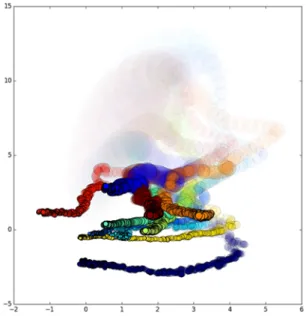
class) during the first epoch of training. The animation is summarized in Fig. 1, where we use a fading effect to describe the evolution in time.
Fig. 1. Trajectories of ten MNIST digist in a binary latent space during the first epoch of training; pictures fade away
with time.
In this case, the network is a simple dense network with layers of dimension 784-256-64-16-2; we shall consider the convolutional case in Section 3.1.
In the figure, each digit is depicted by a circle with an area proportional to its variance. Intuitively, you can think of this area as the portion of the latent space producing a reconstruction similar to the original. At start time, the variance is close to 1, but it rapidly gets much smaller. This is not surprising, since we need to find a place for 60000 different digits. Note also that the ten digits initially have a chaotic distribution, but progressively dispose themselves around the origin in a Gaussian-like shape.
The previous behaviour is the expected one. However, augmenting the number of dimensions of the latent space, we face an interesting phenomenon: the representation becomes sparse.
In Fig. 2 we show the evolution during a typical training of the variance of latent variables in a space of dimension 16 (the rest of network is essentially unchanged).
Table 1 provides relevant statistics for each latent variable at the end of training, computed over the full dataset: the mean of its variance (that we expect to be around 1, since it should be normally distributed), and the mean of the computed variance 2(X)
θ
σ (that we expect to be a small value, close to 0). The mean value is around 0 as expected, and we do not report it.
All variables highlighted in red have an anomalous behavior: their variance is very low (in practice, they
always have value 0), while the variance 2(X)
θ σ
computed by the network is around 1 for each X. In
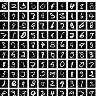
other words, the representation is getting sparse! Only 8 latent variables out of 16 are in use: the other ones are completely ignored by the generator. For instance, in Fig. 3 we show a few digits randomly generated from Gaussian sampling in the latent space (upper line) and the result of generation when inactive latent variables have been zeroed-out (lower line): they are indistinguishable.
Fig. 2. Evolution of the variance along training (16 variables, MNIST case). On the x-axis we have
numbers of minibatches, each one of size 128.
Table 1. Inactive variables in the VAE for generating MNIST digits (dense case, 784-256-64-32-16 architecture).
Fig. 3. Upper line: digits generated from a vector of 16 normally sampled latent variables. Lower line: digits generated after “red” variables have been zeroed-out: these latent variables are completely neglected by the generator.
3.1. Convolutional Case
With convolutional networks, sparsity is less evident. We tested a relatively sophisticated network, whose structure is summarized in Fig. 4; we only describe the encoder; the structure of the decoder is symmetric, upsampling vai transposed Convolutions.
Fig. 4. Architecture of the convolutional encoder. The two final layers compute mean and variance
for 16 latent variables.
The previous network is able to produce excellent generative results (see Fig. 5).
In this case, only 3 of the 16 latent variables are zeroed out. Having less sparsity seems to suggest that convolutional networks make a better exploitation of latent variables, typically resulting in a more precise reconstruction and improved generative sampling. This is likely due to the fact that latent variables encode information corresponding to different portions of the input space, and are less likely to become useless for the generator.
2 Called by some authors aggregate posterior distribution
[17].
Fig. 5. Generation of MNIST digits via a convolutional network.
4. Ensuring KL-divergence is Working
The whole point of VAEs is to force the generator to produce a marginal encoding distribution2( ) = X ( | )
Q z Q z X close to the prior ( )P z . Averaging the Kullback-Leibler regularizer
( ( | ) || ( ))
KL Q z X P z on all input data, and expanding the Kullback-Leibler divergence in terms of entropy, we get: ( | ) ( ) ( ) ( ) . ( | ) ( ( | ) || ( )) = ( ( | )) ( ( | ), ( )) = ( ( | )) ( ) = ( ( | )) ( ) = ( ( | )) ( ( ), ( )) X X X X X z Q z X X z Q z X Cross entropy of Q X vs P z Avg Entropy of Q z X KL Q z X P z Q z X Q z X P z Q z X logP z Q z X logP z Q z X Q z P z − − + − + − + −+ (4)
The cross-entropy between two distributions is minimal when they coincide, so we are pushing Q z( )
towards P z( ). At the same time, we try to augment the entropy of each Q z X( | ); under the usual assumption that Q z X( | ) is Gaussian, this amounts to enlarge the variance, further improving the coverage of the latent space, essential for generative sampling (at the cost of more overlapping, and hence more confusion between the encoding of different datapoints).
If the KL-divergence is working, we expect Q z( )
Let us look at Q z( ) =XQ z X( | ) as a Gaussian
Mixture Model (GMM), and let us consider its moments.
Its first moment (that should be 0) is just the mean over all X of the first moments of the composing distributions Q z X( | ) =N( (μ X),σ2(X)). This means that we expect that the mean of all μ( )X is 0, i.e. the latent space should be centered around the origin.
The variance of Q z( ) (that should be 1) is
(2) (1) 2 (2) (1) 2
( ) = ( ) = ( ) ( )
Var f μ − μ μ X − μ ,
where we use the hat notation to express the mean over all data X.
Under the assumption that μ(1) = 0,
(2) 2 (1) 2 2 2 ( ) = ( ) = ( ) ( ( )) = ( ) , Var f X X X X μ σ μ σ σ + +
where the last passage is again justified by the assumption that μ(1)= 0.
So, if the KL-divergence is properly working, we expect that, for each variable z, the sum between the mean of the variances 2
(X)
σ computed by the network for each X and its actual variance should be 1, that is a condition that can be easily checked.
The reader is referred to [1] for a more thorough investigation of the previous law, together with its experimental validation on many different datasets.
5. KL-divergence and Sparsity
Let us now try to better understand the collapse phenomenon. Let us consider again the loglikelihood for data X.
( | ) ( ( | ) ( ( | ) || ( ))
z Q z Xlog P X z −KL Q z X P z
If we remove the Kullback-Leibler component from the previous objective function, or just keep the quadratic penalty on latent variables, the sparsity phenomenon disappears. So, sparsity must be related to that component, and in particular to the part of the term trying to keep the variance close to 1, that is
2(X) log( 2(X)) 1
θ θ
σ σ
− + + (5)
whose effect typically degrades the distinctive characteristics of the features. It is also evident that if the generator ignores a latent variable, P X z( | ) will not depend on it and the loglikelihood is maximal when the distribution of Q z X( | ) is equal to the prior distribution P z( ), that is just a normal distribution with 0 mean and standard deviation 1. In other words,
the generator is induced to learn a value μθ( ) = 0X , ans a value σθ( ) = 1X ; sampling has no effect, since the sampled value for z will just be ignored.
During training, if a latent variable is of moderate interest for reconstructing the input (in comparison with other variables), the network will learn to give less importance to it; at the end, the Kullback-Leibler divergence may prevail, pushing the mean towards 0 and the standard deviation towards 1. This will make the latent variable even more noisy, in a vicious cycle that will eventually induce the network to completely ignore the latent variable (Fig. 6).
Fig. 6. The vicious cycle leading to latent variable collapse.
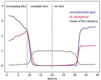
We can get some empirical evidence of the previous phenomenon by artificially deteriorating the quality of a specific latent variable. In Fig. 7 we show the evolution during training of one of the active variables of the variational autoencoder in Table 1 subject to a progressive addition of Gaussian noise. During the experiment, we force the variables that were already inactive to remain so, otherwise the network would compensate the deterioration of a new variable by revitalizing one of the dead ones.
Fig. 7. Evolution of reconstruction gain and KL-divergence of a latent variable during training, acting on its quality by addition of Gaussian blur. We also show in the same picture the evolution of the variance, to compare their progress.
In order to evaluate the contribution of the variable to the loss function we compute the difference between the reconstruction error when the latent variable is zeroed out with respect to the case when it is normally taken into account; we call this information reconstruction gain.
After each increment of the Gaussian noise we repeat one epoch of training, to allow the network to suitably reconfigure itself. In this particular case, the network reacts to the Gaussian noise by enlarging the mean values μx( )X , in an attempt to escape from the noisy region, but also jointly increasing the KL-divergence. At some point, the reconstruction gain of the variable is becoming less than the KL-divergence; at this point we stop augmenting the Gaussian noise. Here, we assist to the sparsity phenomenon: the KL-term is suddenly pushing variance towards 1 (due to equation 5), with the result of decreasing the KL-divergence, but also causing a sudden and catastrophic collapse of the reconstruction gain of the latent variable.
Contrarily to what is frequently believed, sparsity seems to be reversible, at some extent. If we remove noise from the variable, as soon as the network is able to perceive a potentiality in it (that may take several epochs, as evident if Fig. 7), it will eventually make a suitable use of it. Of course, we should not expect to recover the original information gain, since the network may have meanwhile learned a different repartition of roles among latent variables.
6. A Controversial Issue
The sparsity phenomenon in Variational Autoencoders is a controverial topic: you can either stress the suboptimal use of the actual network capacity (overpruning), or its beneficial regularization effects. In this section we shall rapidly survey on the recent research along this two directions.
6.1. Overpruning
The observation that working in latent spaces of sufficiently high-dimension, Variational Autoencoders tend to neglect a large number of latent variables, likely resulting in impoverished, suboptimal generative models, was first made in [4]. The term overpruning to denote this phenomenon was introduced in [24], with a clearly negative acception: an issue to be solved to improve VAE.
The most typical approach to tackle this issue is that of using a parameter to trade off the contribution of the reconstruction error with respect to the Kullback-Leibler regularizer: ( | ) ( ( )) ( ( | ) ( ( | ) || ( )) z Q z X log P X log P X z λKL Q z X P z − ≈ − + (6)
The theoretical role of this lambda-parameter is not so evident; let us briefly discuss it. In the closed form of the traditional logloss fo VAE there are two parameters that seems to come out of the blue, and that may help to understand the λ. The first one is the variance of the prior distribution, that seems to be arbitrarily set to 1. However, as should be clear from the discussion in Section 4, a different variance for the prior may be easily compensated by the learned means
( )X
μ and variances σ2(X)
for the posterior distribution Q z X( | ): in other words, the variance of the prior has essentially the role of fixing a unit of measure for the latent space. The second choice that looks arbitrary is the assumption that the distribution
( | )
P X z has a normal shape around the decoder function d zθ( ): in fact, in this case, the variance of this distribution may strongly affect the resulting loss function, and could justify the introduction of a balancing λ parameter.
Tuning down λ reduces the number of inactive latent variable, but this may not result in an improved quality of generated samples: the network uses the additional capacity to improve the quality of reconstruction, at the price of having a less regular distribution in the latent space, that becomes harder to exploit by a random generator.
More complex variants of the previous technique comprise an annealed optimization schedule for λ [3] or enforcing minimum KL contribution from subsets of latent units [15]. All these schemes require hand-tuning and, to cite [24], they easily risk to “take away the principled regularization scheme that is built into VAE.”
Alternatively, we may try to learn the correct value for λ during training, es e.g. attempted in [7]. The problem, in this case, is the choice of the loss function to minimize: if we use reconstruction error, the network will simply try to neglect the KL-component. The final objective is to maximize the quality of generated samples, but unfortunately there is no clear metrics for that. State of the art proposal for measuring the quality of generated samples, such as Frechet Inception Distance [13] are not accurate enough to be used for balancing between reconstruction error and KL-divergence. We suggest to select a minimal λ large enough to ensure the regularization effect of KL-component, that can be done by checking - either manually or automatically - the laws of Section 4.
A different way to tackle overpruning is that model-based, consisting in devising architectural modifications that may alleviate the problem. For instance, in [25] the authors propose a probabilistic generative model composed by a number of sparse variational autoencoders called epitoms that partially share their encoder-decoder architectures. The intuitive idea is that each data X can be embedded into a small subspace KX of the latent space, specific to the given data.
Similarly, in [8] the use of skip-connections is advocated as a possible technique to address over-pruning.
While there is no doubt that particular network architectures show less sparsity than others (see also the comparison we did in this article between dense and convolutional networks), in order to claim that the aforementioned approaches are general techniques for tackling over-pruning it should be proved that they systematically lead to improved generative models across multiple architectures and many different data sets, that is a result still in want of confirmation.
6.2. Regularization
Recently, there have been a few works trying to stress the beneficial effects of the Kullback-Leibler component, and its essential role for generative purposes.
An interesting perspective on the calibration between the reconstruction error and the Kullback-Leibler regularizer is provided by β-VAE [14] [5]. Formally, the shape of the objective function is the same of equation 6 (where the parameter λ is renamed β ), but in this case the emphasis is in pushing β to be high. This is reinforcing the sparsity effect of the Kullback-Leibler regularizer, inducing the model to learn more disentangled features. The intuition is that the network should naturally learn a representation of points in the latent space such that the “confusion” due to the Kullback-Leibler component is minimized: latent features should be general, i.e. apply to a large number of data, and data should naturally cluster according to them. A metrics to measure the degree of disentanglement learned by the model is introduced in [14], and it is used to provide experimental results confirming the beneficial effects of a strong regularization. In [5], an interesting analogy between β-VAE and the Information Bottleneck is investigated.
In a different work [6], it has been recently proved that a VAE with affine decoder is identical to a robust PCA model, able to decompose the dataset into a low-rank representation and a sparse noise. This is extended to the nonlinear case in [7]; in particular, it is proved that a VAE with infinite capacity can detect the manifold dimension and only use a minimal number of latent dimensions to represent the data, filling the redundant dimensions with white noise. In the same work the authors propose a quite interesting two stage approach, to address the potential mismatch between the aggregate posterior Q z( ) and the prior ( )P z : a second VAE is trained to learn an accurate approximantion of Q z( ); samples from a Normal distribution are first used to generate samples of Q z( ), and then fed to the actual generator of data points. In this way, it no longer matters that ( )P z and
( )
Q z are not similar, since you can just sample from
the latter using the second-stage VAE. This approach does not require additional hyperparameters or sensitive tuning, and produces high-quality samples, competitive with state-of-the-art GAN models, both in terms of FID score and visual quality.
7. Conclusions
In this article we discussed the interesting collapse phenomenon for latent variables typical of Variational Autoencoders, and briefly surveyed some of the recent literature on the topic. Our point of view is slightly different from the traditional overpruning perspective, in the sense that maybe, as it is also suggested in other recent works (see Section 6.2), there is no issue to tackle: the Kullback-Leibler component has a beneficial self-regularizing effect with all the advantages tipically associated with sparsity: it forces the model to focus on the really important and more disentangled features, sensibly reducing the risk of overfitting.
This suggests a very clear methodology that can be followed for training VAEs. First of all, we must correctly balance the KL component, ensuring it is properly working, by checking the first moments of the latent distribution or also, as suggested in Section 4, the fact that for each latent variable, the sum between its variance and the average variance of the Gaussian distributions ( |Q z X) is always approximately 1 . Then, we progressively augment the dimension of the latent space to attain sparsity. If the resulting network does not give satisfactory generative results, we should likely switch to more sophisticated architectures, making a better exploitation of the latent space. Finally, if the reconstruction error is low but generation is bad, it is a clear indication of a mismatch between the aggregate posterior Q z( ) and the prior
( )
P z ; in this case, a simple two-stage approach as described in [7] might suffice to solve the issue.
References
[1]. Andrea Asperti, About generative aspects of variational autoencoders, in Proceedings of the 5th International Conference on Machine Learning, Optimization, and Data Science, September 10-13, 2019, Certosa di Pontignano, Siena, Tuscany, Italy, LNCS (to appear). 2019.
[2]. Andrea Asperti, Sparsity in variational autoencoders, in Proceedings of the 1st International Conference on Advances in Signal Processing and Artificial Intelligence (ASPAI 2019), Barcelona, Spain, 20-22 March, 2019, pp. 11-22.
[3]. Samuel R. Bowman, Luke Vilnis, Oriol Vinyals, Andrew M. Dai, Rafal Józefowicz, and Samy Bengio, Generating sentences from a continuous space, in Proceedings of the SIGNLL Conference on Computational Natural Language Learning (CONLL), 2016, abs/1511.06349.
[4]. Yuri Burda, Roger B. Grosse, and Ruslan Salakhutdinov, Importance weighted autoencoders. in Proceedings of the ICLR 2015 Conference, abs/1509.00519.
[5]. Christopher P. Burgess, Irina Higgins, Arka Pal, Loic Matthey, Nick Watters, Guillaume Desjardins, and Alexander Lerchner, Understanding disentangling in beta-vae, in Proceedings of the NIPS Workshop on Learning Disentangled Representations, 2017. [6]. Bin Dai, Yu Wang, John Aston, Gang Hua, and David
P. Wipf, Connections with robust PCA and the role of emergent sparsity in variational autoencoder models, Journal of Machine Learning Research, 19, 41, 2018, pp. 1-42.
[7]. Bin Dai and David P. Wipf, Diagnosing and enhancing vae models, in Proceedings of the 7th International Conference on Learning Representations (ICLR 2019), May 6-9, New Orleans, 2019.
[8]. Adji B. Dieng, Yoon Kim, Alexander M. Rush, and David M. Blei, Avoiding latent variable collapse with generative skip model, in Proceedings of the 22nd International Conference on Artificial Intelligence and Statistics (AISTATS’ 2019), Naha, Okinawa, Japan, 2019, abs/1807.04863.
[9]. Carl Doersch. Tutorial on variational autoencoders. CoRR, abs/1606.05908, 2016.
[10]. S. M. Ali Eslami, Danilo Jimenez Rezende, Frederic Besse, Fabio Viola at all, Neural scene representation and rendering, Science, 360, 6394, 2018, pp. 1204– 1210.
[11]. Ian Goodfellow, Yoshua Bengio, and Aaron Courville, Deep Learning, MIT Press, 2016.
http://www.deeplearningbook.org
[12]. Karol Gregor, Ivo Danihelka, Alex Graves, and Daan Wierstra, DRAW: A recurrent neural network for image generation, in Proceedings of the 32nd International Conference on Machine Learning, Lille, France, 2015, abs/1502.04623.
[13]. Martin Heusel, Hubert Ramsauer, Thomas Unterthiner, Bernhard Nessler and Sepp Hochreiter, Gans trained by a two time-scale update rule converge to a local nash equilibrium, in Proceedings of the Advances in Neural Information Processing Systems 30: Annual Conference on Neural Information Processing Systems, 4-9 December 2017, Long Beach, CA, USA, pp. 6629–6640.
[14]. Irina Higgins, Loic Matthey, Arka Pal, Christopher Burgess, Xavier Glorot, Matthew Botvinick, Shakir Mohamed, and Alexander Lerchner, Beta-vae: Learning basic visual concepts with a constrained variational framework, in Proceedings of the 5th International Conference on Learning Representations (ICLR’17), 2017.
[15]. Diederik P. Kingma, Tim Salimans, and Max Welling, Improving variational inference with inverse autoregressive flow, in Proceedings of the 29th
Conference on Neural Information Processing Systems (NIPS 2016), Barcelona, Spain, CoRR, abs/1606.04934, 2016.
[16]. Diederik P. Kingma and Max Welling, Auto-encoding variational bayes, in Proceedings of the ICLR 2014 Conference, 2014, abs/1312.6114.
[17]. Alireza Makhzani, Jonathon Shlens, Navdeep Jaitly, and Ian J. Goodfellow, Adversarial autoencoders, in Proceedings of the International Conference on Learning Representations, 2016,abs/1511.05644. [18]. Tom Rainforth, Adam R. Kosiorek, Tuan Anh Le,
Chris J. Maddison, Maximilian Igl, Frank Wood, and Yee Whye Teh. Tighter variational bounds are not necessarily better, in Proceedings of the 35th International Conference on Machine Learning, ICML 2018, Stockholmsmässan, Stockholm, Sweden, July 10-15, 2018, Vol. 80, pp. 4274–4282.
[19]. Danilo Jimenez Rezende, Shakir Mohamed, and Daan Wierstra, Stochastic backpropagation and approximate inference in deep generative models, in Proceedings of the 31th International Conference on Machine Learning (ICML 2014), Beijing, China, 21-26 June 2014, Vol. 32, pp. 1278–1286.
[20]. Kihyuk Sohn, Honglak Lee, and Xinchen Yan, Learning structured output representation using deep conditional generative models, in Advances in Neural Information Processing Systems (C. Cortes, N. D. Lawrence, D. D. Lee, M. Sugiyama, and R. Garnett, Eds.), Curran Associates, Inc., 28, 2015, pp. 3483–3491.
[21]. Jacob Walker, Carl Doersch, Abhinav Gupta, and Martial Hebert, An uncertain future: Forecasting from static images using variational autoencoders, in Proceedings of the European Conference on Computer Vision (ECCV 2016), 2016, pp 835-851, abs/1606.07873.
[22]. Jacob Walker, Carl Doersch, Abhinav Gupta, and Martial Hebert, An uncertain future: Forecasting from static images using variational autoencoders, in Proceedings of the 14th European Conference on Computer Vision (ECCV 2016), Amsterdam, The Netherlands, October 11-14, 2016, LNCS, Vol. 9911, pp. 835–851.
[23]. Raymond A. Yeh, Ziwei Liu, Dan B. Goldman, and Aseem Agarwala. Semantic facial expression editing using autoencoded flow, CoRR, abs/1611.09961, 2016.
[24]. Serena Yeung, Anitha Kannan, Yann Dauphin, and Li Fei-Fei. Tackling over-pruning in variational autoencoders, in Proceedings of the Workshop on Principled Approaches to Deep Learning (ICML 2017), 2017, abs/1706.03643.
[25]. Serena Yeung, Anitha Kannan, and Yann Dauphin, Epitomic variational autoencoder, Submited to ICLR 2017 Conference, 2017.
https://openreview.net/pdf?id=Bk3F5Y9lx __________________
Published by International Frequency Sensor Association (IFSA) Publishing, S. L., 2019 (http://www.sensorsportal.com).