This is a repository copy of Geometry of Uncertainty Relations for Linear Combinations of Position and Momentum.
White Rose Research Online URL for this paper: http://eprints.whiterose.ac.uk/124593/
Version: Accepted Version
Article:
Kechrimparis, Spyridon and Weigert, Stefan Ludwig Otto orcid.org/0000-0002-6647-3252 (2017) Geometry of Uncertainty Relations for Linear Combinations of Position and
Momentum. Journal of Physics A: Mathematical and Theoretical. 025303. ISSN 1751-8113 https://doi.org/10.1088/1751-8121/aa9cfc
[email protected] https://eprints.whiterose.ac.uk/ Reuse
Items deposited in White Rose Research Online are protected by copyright, with all rights reserved unless indicated otherwise. They may be downloaded and/or printed for private study, or other acts as permitted by national copyright laws. The publisher or other rights holders may allow further reproduction and re-use of the full text version. This is indicated by the licence information on the White Rose Research Online record for the item.
Takedown
If you consider content in White Rose Research Online to be in breach of UK law, please notify us by
Geometry of Uncertainty Relations for
Linear Combinations of Position and Momentum
Spiros Kechrimparis
a∗and Stefan Weigert
b†November 9, 2017
aDepartment of Applied Mathematics, Hanyang University (ERICA)
55 Hanyangdaehak-ro, Ansan, Gyeonggi-do, 426-791, Korea
bDepartment of Mathematics, University of York
York, YO10 5DD, United Kingdom
Abstract
For a quantum particle with a single degree of freedom, we derive preparational sum and product uncertainty relations satisfied byNlinear combinations of position and mo-mentum observables. The bounds depend on theirdegree of incompatibilitydefined by the area of a parallelogram in anN-dimensional coefficient space. Maximal incompatibility occurs if the observables give rise to regular polygons in phase space. We also conjecture a Hirschman-type uncertainty relation forNobservables linear in position and momen-tum, generalizing the original relation which lower-bounds the sum of the position and momentum Shannon entropies of the particle.
1
Introduction
For a long time, quantum mechanical uncertainty relations were tantamount to statements aboutpairsof non-commuting observables. Heisenberg’s discussion of a fictitiousγ-ray mi-croscope in 1927 [1] led Kennard to immediately derive a rigorouspreparationaluncertainty relation [2] for the product of the variances of position and momentum observables. The existence of pairwise incompatible observables represents one of the defining features of quantum theory.
It is natural to suspect that similar limitations may also exist for triples, quadruples, etc. of non-commuting observables, and they may not be reducible to uncertainty relations for pairs. Indeed, the triple uncertainty relation [3], for example,
∆p∆q∆r≥
τh¯ 2
3/2
, τ =csc
2π 3
≃1.15 , (1)
bounds the product of the variances ofthree pairwise canonicaloperators, ˆp, ˆq, and ˆr=−pˆ−qˆ. The bound (1) follows neither from individually applying Heisenberg’s uncertainty relation
to each of the canonical pairs of observables(pˆ, ˆq), (qˆ, ˆr) and(rˆ, ˆp), nor from its generaliza-tion found by Robertson and Schr ¨odinger [4, 5]. Early on, Robertson derived inequalities for sets of more than two observables [6] but the results do not cover the situation we will consider. For example, his bound on the product of the variances of the observables ˆp, ˆq, and ˆrturns out to be the trivial one,∆p∆q∆r ≥0.
For a long time, uncertainty relations for continuous variables were thought to be of mainly conceptual interest. For systems with more than one degree of freedom, however, they are now known to provide tools to detect entanglement. The criteria may, for example, either use the variances of position and momentum operators only, as in [7], or the entire covariance matrix [8]. Not surprisingly, the triple uncertainty relation (1) also lends itself to detect entanglement, according to a recent proposal and its quantum optical realization [9].
In this paper, we will derive tight inequalities for the product and the sum of variances of finitely many observables for a single continuous variable describing, for example, a quan-tum particle restricted to move on the real line. We limit ourselves to linear combinationsof position and momentum observables. Recent work on uncertainty relations beyond pairs of observables [10, 11] has led to new state-dependent bounds, as well as to bounds on the variances of multipleunitaryoperators [12]. In contrast to these approaches, thelinearityof the observables we consider will lead tostate-independentbounds, for the traditional case of Hermitean observables.
We will also introduce a many-observable generalization of theentropicuncertainty rela-tion conjectured by Hirschman [13] in 1957 (but proved only two decades later [14, 15]). It is, in fact, straightforward to ask for a bound on the sum ofmore than twoShannon entropies for a given quantum state. As for variance-based uncertainty relations, we again expect Gaus-sian states to play an important role, suggested by the fact that theysaturatethe proposed inequalities. Recent results for entropic uncertainty relations valid in Hilbert spaces of small finite dimensions show how difficult it is to obtain tight bounds [16].
We have laid out this paper in the following way. In Sec. 2 we derive inequalities obeyed by the variances of N observables linear in position and momentum. The “non-commutativity” encoded in their pairwise commutators can be expressed in the degree of incompatibility, i.e. a real number which determines the lower bounds on sums and products of variances. Geometrically, this degree is given by the area of a suitably defined parallelo-gram in coefficient spaceRN. Specific sets of observables associated with regular polygons are shown to saturate the bounds. In Sec. 3 we generalize Hirschman’s entropic uncertainty relation to more than two observables and explain why we expect the conjectured bounds to be tight. The last section summarizes our results and we will draw conclusions.
2
Variance-based uncertainty relations
The position and momentum observables ˆpand ˆqof a single quantum particle act on Hilbert space the elements of which can be represented as square-integrable functions over the real line, i.e. H =L2(R). We introduceNHermitean operators by combining them linearly,
ˆ
rj =ajpˆ+bjqˆ, aj,bj ∈ R, j =1 . . .N. (2)
by a vector in a two-dimensional Euclidean space,
rj =
aj bj
∈ R2, j=1 . . .N. (3)
We will callrj =qa2j +b2j the “length” of the observable ˆrj. The fundamental commutation relation
[pˆ, ˆq] = ¯h
iIˆ (4)
where ˆI is the the identity operator on the Hilbert spaceH , implies that the pairwise
com-mutators of ther-observables are given by
ˆ
rj, ˆrk = A(rj,rk)h¯
iIˆ, j,k =1 . . .N, (5)
with the function A(·,·) computing the (signed) area of the parallelogram determined by the vectorsrj,rk ∈R2,
A(rj,rk) = ajbk−akbj≡ Ajk. (6) Thus, the commutation relations between the r-observables are encoded in the N-by-N
skew-symmetric matrix A with matrix elements Ajk = −Akj. This antisymmetric struc-ture finds its natural expression in a coordinate-independent formulation. Let us treat the linear combinations ˆrj, j=1 . . .N, as components of a vector operator with Ncomponents,
ˆ r=
ˆ
r1
... ˆ
rN
≡apˆ+bqˆ, a,b∈ RN. (7)
Since the components of the exterior product of two vectorsu,v∈ RN, are given by
(u∧v)jk =ujvk−ukvj, j,k=1 . . .N, (8)
we find that the N2commutation relations (5) elegantly combine to
ˆ
r∧ˆr= a∧bh¯
i Iˆ. (9)
Normally, the wedge product of a vector with itself is equal to zero but this does not apply to the left-hand-side of (9) because ˆr is a vector with operator-valued, non-commuting compo-nents. The relation is consistent with writing ˆr=∑Nj=1rˆjej, where the vectorsej, j=1 . . .N,
form the standard orthonormal basis of the space RN, and using the anti-symmetry of the exterior productsej∧ek =−ek∧ej. In a similar spirit, the commutation relations for a spin,
∑qrεpqrsˆqsˆr =isˆp, p,q,r ∈ {x,y,z}, can be written formally as a cross product, ˆs×sˆ = i¯hsˆ, by combining the three operator-valued components of a quantum spin in a single vec-tor ˆs = ¯h
2σˆ (see [20], for example). It will be useful to write Eq. (8) in vector form, i.e. u∧v=u⊗v−v⊗u, where the outer productu⊗vof two vectors is defined by
(u⊗v)jk ≡uvT
jk , j,k=1 . . .N. (10)
|a∧b|2 =
N
∑
j>k=1A2jk. (11)
It has a simple expression in terms of the vectors defining ther-operators,
|a∧b|2=
N
∑
j>k=1ajbk−akbj
2
=|a|2 |b|2−(a·b)2 , (12)
which follows from Lagrange’s identity for real numbers. Usinga·b =|a| |b|cosφ, where φ∈ [0,π)is the angle between the vectorsaandb, one finds
|a∧b| =|a| |b|sinφ, (13)
in agreement with the wedge product being a generalization of the vector product inR3. Geometrically, the squared norm of a bi-vectora∧bis given by the sum of the squared areas of the parallelograms defined by all pairs of vectors rj ∈ R2, j = 1 . . .N, which,
ac-cording to (12), equals the square of the area of the parallelogram spanned by the vectors a,b ∈ RN in coefficient space. Not surprisingly, the norm is also closely related to a norm of the antisymmetric matrix A defined by Eq. (5): the square of its Frobenius (or Hilbert-Schmidt orL2,2)norm reads
kAk2F =Tr
ATA=
N
∑
j,k=1A2jk =2
N
∑
j>k=1A2jk =2|a∧b|2 . (14)
This relation will be used in Sec. 2.3
2.1
Sum and product inequalities
The variances ∆2r
j ≡ hψ|rˆ2j|ψi − hψ|rˆj|ψi2 of the N linearly dependent r-observables in a
pure state|ψi ∈H are given by
∆2rj =a2j∆2p+b2j∆2q+2ajbjCpq, j=1 . . .N, (15)
where we have introduced the covariance
Cpq = 1
2(hψ|(pˆqˆ+qˆpˆ)|ψi − hψ|pˆ|ψihψ|qˆ|ψi) . (16) Adding the variances∆2rj, we obtain
N
∑
j=1∆2rj =|a|2∆2p+|b|2∆2q+2a·bCpq. (17)
The right-hand-side of Eq. (17) defines a functional of three operators quadratic in position and momentum. The bounds of such expressions have been studied systematically in [21]. An explicit, non-trivial lower bound has been obtained for the linear combination of the variances∆2p,∆2qand the covarianceC
pq (see Eq. (72) of [21]),
µ∆2p+ν∆2q+2λCpq ≥h¯ q
This inequality follows directly and elegantly from the non-negative expectation value of a quadratic form in position and momentum in an arbitrary quantum state ˆρ,
Trhzˆρˆzˆ†i=Tr
ˆ
zρˆ1/2 zˆρˆ1/2†
≥0 , (19)
where
ˆ
z =α(pˆ− hpˆi) +β(qˆ− hqˆi) , hpˆi ≡ Tr[ρˆpˆ] , etc. , (20) andα,β ∈ R, are complex numbers which satisfy Im(α β∗) ≥0. A straightforward calcula-tion shows that upon identifyingµ ≡ |α|2,ν = |β|2 and λ = Re(α∗β) one obtains indeed (18), valid for both pureandmixed states.
Setting
µ≡ |a|2, ν≡ |b|2, λ≡a·b, (21)
we can apply the tight inequality (18) since |a|2,|b|2 > 0 and|a|2|b|2 > (a·b)2 hold.
Re-calling the identity (12) leads to thesum inequalityfor arbitrary quantum states,
N
∑
j=1∆2rj ≥¯h|a∧b| , (22)
which is our first main result. Appendix A presents an alternative derivation which is based on the validity of (18) for pure states and the concavity of the variance.
Eq. (22) correctly reproduces both the pair and triple sum identities leading to the bounds ¯
h and ¯h√3, respectively. The bound is state-independent because the commutator between any two linear combinations of position and momentum is a scalar multiple of the identity. A trivial bound (zero) is obtained if the inequality (18) is applied to each term of the sum (17) separately, i.e.beforeinstead ofafterthe summation in (17).
Using (5) it is possible to express the lower bound of the inequality (22) in terms of the pairwise commutators between theN operators,
N
∑
j=1∆2rj
!2
≥
N
∑
j>k=1
h[rˆj, ˆrk]i2 , (23)
where the expectation values of the commutators are taken in the state|ψi. Thus, the sum of the variances of N different linear combinations ˆrj of position and momentum operators is
seen to be bounded from below by the square root of thesum of the modulus squared of all com-mutators between the operators. Applying the Cauchy-Schwarz inequality to this expression forN >2, we find that
N
∑
j>k=1
h[ˆrj, ˆrk]i2 > 1
N−1
N
∑
j>k=1
h[ˆrj, ˆrk]i
!2
. (24)
Upon concatenating this inequality with (23), we obtain a bound on the sum of Nvariances which can be derived directly from the inequalities valid for each of the N(N−1) pairs (∆2r
k+∆2rj), 1≤k< j≤ N. The stronger bound (22) shows that these uncertainty relations
To identify the states saturating the inequality (22) let us introduce the ground state |0i
of a harmonic quantum oscillator with unit mass and frequency, and the family of coherent states|αi= Tˆα|0i, where the unitary operator
ˆ
Tα =exp[i(p0qˆ−q0pˆ)/¯h] , α = √1
2¯h(q0+ip0) , (25)
generates a position and momentum translation by amountsq0 and p0. As shown in [21],
the inequality (18) and hence the sum inequality (22) attain their minimum if the oscillator resides in a suitablysqueezedground state|0i,
|µ,ν,λi =Gˆλ ν
ˆ
S
1
2ln √ ν
µν−λ2
!|0i, (26)
or in any state obtained from rigidly displacing it, i.e. ˆTα|µ,ν,λi. Here, the unitary operator
ˆ
Gg =exp
h
igpˆ2/2¯hi , g∈ R, (27)
generates amomentum gaugetransformation while ˆ
Sγ =exp[iγ(qˆpˆ+pˆqˆ)/2¯h] , γ∈ R, (28)
squeezesa state along the coordinate axes of phase space. ForN =2, with observables ˆr1 = pˆ
and ˆr2 = qˆ, say, corresponding toµ = ν = 1 andλ = 0, we find ˆG0 = Sˆ0 = Iˆ. This result agrees with the well-known fact that the only states minimizing the sum∆2p+∆2qare given
by the ground state of a harmonic oscillator and its rigid displacements in phase space. Next, we wish to generalize Heisenberg’s uncertainty relation by deriving a bound on the value of theproductof the variances for the observables ˆrj,j=1 . . .N,
J[|ψi] =
N
∏
j=1∆2rj, (29)
where N ≥2. Using the identities (15), the functional J[|ψi], which associates a number to each state |ψi, turns into a polynomial of order N in the basic variances ∆2p,∆2q, and the
covariance Cpq. Its lower bound could be determined by applying the method described
in [21]. However, in this highly symmetric case, another method turns out to be simpler which enables us to minimize the product J while respecting the constraint given by the sum inequality (22).
A function J(~x) has a minimum in the presence of an inequalityg(~x) ≤ 0 if the
Karush-Kuhn-Tucker (KKT) conditions [25] are satisfied,
∂J(~x)
∂xj +κ
∂g(~x)
∂xj =0 , j=1 . . .N, (30)
κg(~x) = 0 , (31)
where κ is a positive constant yet to be determined. Identifying the variables xj with the variances∆2rj,j = 1 . . .N, the constraint (22) reads g(~x) ≡ c−∑
jxj ≤ 0, with the positive
numberc =h¯ |a∧b|.
The unique solution of the KKT conditions (30) is easily found to be
x1 =x2 =. . . =xN =
c
which implies that the smallest value of the functional J[|ψi] is given by(c/N)N. In terms of the original variables, we finally obtain theproduct inequalityfor the variances ofNlinear combinations of position and momentum,
N
∏
j=1∆2rj ≥
¯
h|a∧b|
N
N
, (33)
our second main result. The lower bounds for Heisenberg’s uncertainty relation and for the triple product uncertainty relation (1) are reproduced correctly. The bounds are symmetric in all pairs of the N observables ˆrj,j = 1 . . .N, and they display a neat structure which involves the exterior product of the momentum and position coefficients inRN. The result (33) is genuinely different from Robertson’s inequalities for Nobservables [6] since already in the case ofN =3 only a trivial bound results,∆p∆q∆r ≥0. In addition, the derivation of inequality (33) also applies to mixed states, i.e.∆2r
j =Tr
ˆ
ρrˆ2j− Tr ˆρrˆj2,j =1 . . .N.
2.2
Regular polygons
Let us now determine the bounds for N observables arranged in a symmetric way. We assume that the tips of the vectors rj ∈ R2,j = 1 . . .N, are located on a circle of radius
R∈ (0,∞), and that they are distributed homogeneously. Explicitly, we have
ˆ
rj = Rcosϕjpˆ+ Rsinϕjqˆ, ϕj = 2π(j−1)
N , j=1, . . . ,N. (34)
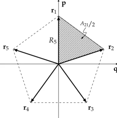
The tips of the vectors define a regular polygon withNvertices in the spaceR2, as illustrated in Fig. (1). We will always align the first observable with the momentum operator, i.e. ˆ
r1 = Rpˆ. This choice is not a restriction since the commutation relations do not change under rotations inR2(cf. Appendix B).
From a structural point of view, the value of the constant R is not important as it only rescales all observables. One natural choice to fix this scale is to require that any two adjacent observables form a canonical pair,
[ˆrj, ˆrj+1] = h¯
i Iˆ, rˆN+1 ≡rˆ1, j =1 . . .N. (35)
These conditions are satisfied if the circumradiusRof the polygon takes the value
RN = √ 1
sin∆N , ∆N = 2π
N . (36)
In this case, the parallelograms defined by any two consecutive vectors rj and rj+1, which
enclose the angle 2π/N, have unit area area, A(rj,rj+1) = 1. As the angles between
neigh-bouring vectors decrease with larger values of N, the circumradius of the polygon must increase asRN ≃
√
Nin order to ensure (35).
Since the coefficient vectorsaandbhave components
aj =RNcosϕj, bj =RNsinϕj, j =1 . . .N, (37)
we find that
|a∧b|= NR
2 N
2 ≡
N
r1
R5
A21/2
r5
r4 r3
r2 p
[image:9.595.199.393.30.225.2]q
Figure 1: A regular pentagon in the dimensionless “phase space” R2, associated with the canonical operators ˆrj,j = 1 . . . 5, introduced in (34), of circumradius R5 = 1/
p
sin(2π/5) (cf. Eq. (36)) and with area A = 5/2. The shaded triangle has half the size of the area
A21 ≡ A(r2,r1) ≡ 1 given by the parallelogram spanned by the vectors r2 and r1 (cf. Eq.
(6)).
Here we have used the trigonometric identities
N
∑
j=1sin2
2πj N = N 2 and N
∑
j=1 sin4πj N
=0 , (39)
to show that
|a|2 =|b|2 = NR
2 N
2 and a·b=0 , (40)
respectively. Now the identity (12) implies that the sum and the product inequalities (see Eqs. (22) and (33)) for the variances of N observables associated with regular polygons are given by
N
∑
j=1∆2rj ≥ N¯h
2 sin∆N and
N
∏
j=1∆2rj ≥
¯
h
2 sin∆N
N
, (41)
respectively .
It is possible to absorb the factor sin∆N on the right-hand-side of these inequalities by considering vectorsrjin (34) with tips located on theunitcircle. In this case, the
right-hand-side of the commutators (35) is found to be proportional to sin∆N ≃ 1/√N since adjacent observables differ less and less for increasing values of N. Then, the bounds in Eqs. (41) take particularly simple forms,
N
∑
j=1∆2rj ≥N h¯
2 and
N
∏
j=1∆2rj≥ ¯ h 2 N , (42)
i.e. each variance formally contributes at least an amount ¯h/2. The states that saturate these inequalities are the coherent states |αi = Tˆα|0i, introduced via Eq. (25). If N = 2 or
2.3
Degrees of incompatibility
In this section, we will argue that the dependence of the sum and product bounds on only the norm|a∧b|is not a coincidence. We will show that there exists a transformation which maps the vector operator ˆr =aqˆ+bpˆto ˆr′ =a′qˆ+b′pˆ in such a way that the commutation relations (9) assume theirstandard form,
ˆ
r′∧ˆr′ =|a∧b| e1∧e2h¯
iIˆ, (43)
where e1 and e2 are a pair of orthogonal unit vectors in the coefficient space RN.
There-fore, the commutation relations forNlinear combination of position and momentum can be characterized by a single real number,
Inc(a,b) ≡ |a∧b| , (44)
measuring the degree of incompatibility of the observables ˆrj, j = 1 . . .N. The relation (43) states that the original commutation relations are equivalent to a situation in which all but two ˆr-observables have been mapped to 0,
ˆ
r1′ =|a∧b|1/2pˆ, rˆ′
2 =|a∧b|1/2qˆ, rˆk′ =0 , k=3 . . .N, (45)
corresponding to
a′ =|a∧b|1/2e
1 and b′ =|a∧b|1/2e2, (46)
respectively. We will obtain the standard form (43) by exploiting the fact that the norm of the bi-vectora∧b is invariant under (i) gauge transformations and under (ii) transformations of the vector operator ˆrwhich are orthogonal inRN.
Before embarking on this calculation, we mention that other measures of incompatibility forpairsof observables exist. Thejoint measurability region[26] quantifies the incompatibility of two observables based on the amount of noise that needs to be added in order for them to become jointly measurable. Based on this notion a coarser measure can be introduced, the joint measurability degree [27], which returns a real number between 1/2 (correspond-ing to maximal incompatibility) and 1 (compatibility). For continuous variables, the pair of position and momentum is found to be maximally incompatible which agrees with the measure Inc(a,b)introduced here. However, the case of three or more observables has not been considered
To derive the relations (43), we first note that the observables
ˆ
rU =Uˆ rˆUˆ†, (47)
obtained from ˆrby any unitary operator ˆU, satisfy the same commutation relations as the original observables ˆr. If we limit ourselves tolinear canonical transformations of the ob-servables ˆq and ˆp, we find a set of transformations forming the group Sp(2,R), generated by rotations, squeeze and gauge transformations described in [28].
Taking the unitary ˆU = Gˆg as defined in Eq. (27), position and momentum operators
transform according to
ˆ
pg= pˆ,
ˆ
Clearly, the transformed coordinate vectors areag =aandbg =b+ga. The components of
the vector operator ˆrg have the same commutators as those of ˆras follows from the
proper-ties of the exterior product,
ag∧bg=a∧(b+ga) = a∧b. (49)
Geometrically, the parameter g labels a continuous family of parallelograms with sides ag
andbg. They all have the same area as they are related to each other by a shear
transforma-tion. If the parametergtakes the value
g⊥ =−a·b
|a|2 , (50)
the parallelogram turns into a rectangle spanned by two orthogonal vectors, a⊥ = a and b⊥ =b+g⊥a.
The right-hand-side of the commutation relations ˆr⊥∧ˆr⊥ = i¯ha⊥∧b⊥Iˆnow depends on the orthogonal vectorsa⊥ and b⊥. Denote unit vectors aligned with them byea and eb,
respectively, and consider an orthogonal transformation R, i.e. RRT = RTR = I, which rotates the vector operator ˆr⊥into
ˆ
r′ =Rˆr⊥. (51)
Note that, typically, such a transformationcannotbe generated by a unitary operator acting on the fundamental pair ˆp and ˆq. Sinceea·eb = 0, we can always find a transformation R
which maps the vectorseaandebto the first two elements of the standard basis,
ea =Re1, eb =Re2. (52)
The rotationRis unique only forN =3 since inR3the map of the vectorse
1and e2
deter-mines the fate of the third basis vector, via e3 = e1×e2. Using the definition of the outer
product in (10) and the fact thatR−1=RT, one finds that
(Ra)⊗(Rb) = (Ra) (Rb)T =RabTRT, (53)
so that the exterior product (8) transforms according to
(Ra)∧(Rb) = RabT−baTRT ≡R(a∧b)RT. (54)
The relation (14) now implies that the length of the bi-vector a∧b is invariant under any rotationRapplied to theN-component vector operator ˆr,
|(Ra)∧(Rb)|2 = 1 2Tr
RARTTRART= 1 2Tr
ATRTR A RTR=|a∧b|2. (55)
Applying this property to the vector operator ˆr′ = R(a⊥pˆ+b⊥qˆ), we finally obtain the desired result, Eq. (43). In general, the vectorsa⊥ andb⊥ will be of different lengths. There is, however, a squeeze transformation which rescales the pair ˆq, ˆp, such that the lengths of the vectors will be equal (see Appendix B).
2.4
Maximal incompatibility
compatible, Inc(a,λa) = 0, for allλ ∈ R. Multiplying the operators ˆr
j by a common factor
λ ∈R, rescales their incompatibility accordingly,
Inc(λa,λb) = λInc(a,b). (56)
To avoid artificially inflated values of incompatibility, it is natural to require that the vectors rjwhich fix the operators ˆrj, j=1 . . .N, have at most length one,
|rj|2≡rj2≤1 , j =1 . . .N. (57)
This constraint is consistent with Heisenberg’s uncertainty relation for the canonically con-jugate pair of position and momentum observables.
It makes sense to ask for themaximalvalue which the incompatibility Inc(a,b) = |a∧b|
may take for N observables ˆr. The maximum is of interest because it will determine the largest possible bounds for the sum and the product inequalities, by “exhausting” the quan-tum mechanical non-commutativity of the observables. Suppose we are givenNobservables defined by the vectorsrj =rjuj, j=1 . . .N, where eachujis a unit vector and the lengthsrj
satisfy (57). Then, the estimate
Inc2(a,b) =
N
∑
j>k=1A2(rj,rk) = N
∑
j>k=1r2jr2kA2(uj,uk)≤ N
∑
j>k=1A2(uj,uk) (58)
shows that their incompatibility is smaller than that of N observables associated with the vectorserj = uj, with all their tips located on the unit circle. Thus, maximal incompatibility
will necessarily arise for an arrangement ofN points on the unit circle.
It is instructive to discuss the simple case of N = 2. Position ˆq and momentum ˆpsatisfy Heisenberg’s uncertainty relation and should, of course, provide an example of maximal incompatibility. The incompatibility of any two observables with vectorsrj = rjuj,j = 1, 2, satisfying (57) and withu1·u2 =cosφ, is given by
Inc2(a,b) ≡(a1b2−a2b1)2 =r21r22sin2φ≤1 . (59)
It achieves its maximum forr1 =r2=1 andφ=±π/2. Thus, the pairs(qˆ,±pˆ)and all those obtained from rotating them by an angleθ ∈ [0, 2π) indeed max out the non-commutativity. The vectors a and b are necessarily orthogonal and of equal length. If the pair (u1,u2)
describes a configuration with maximal incompatibility, then all four configurations with vectors(±u2,±u2)are also maximally incompatible. We ignore the uncertainty- preserving
squeeze transformations here since they do not have an equivalent for other values ofN. Let us now search for the arrangements of not just two but N vectors with tips on the unit circle which will result in maximal incompatibility. Using the identity (12), we find
Inc(a,b) = |a| |b|sinφ, φ∈[0,π), (60)
where the angle between the two vectors inRNis defined by the relationa·b=|a| |b|cosφ. Summing the conditionsr2j = a2j +b2j = 1, j = 1 . . .N, over all values of j, one finds|b|2 =
N− |a|2which implies
Inc(a,b) = |a|
q
N− |a|2 sinφ≤ |a|qN− |a|2≤ N
2 . (61)
The last inequality follows because the function f(x) = x√N−x2has its unique maximum
p
q r1
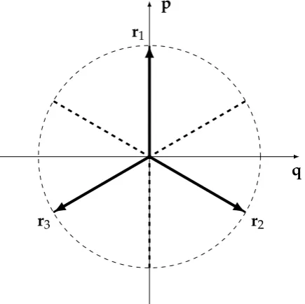
[image:13.595.188.406.32.249.2]r3 r2
Figure 2: Phase-space visualization of three maximally incompatible observables: each of the eight triples(±r1,±r2,±r3)corresponds to observables which maximise the
incompati-bility Inc(a,b)since the variances∆rˆj are invariant under ˆrj → −rˆj, j =1, 2, 3. In addition,
each configuration may be rotated rigidly by any angle between 0 and 2π/3 without chang-ing the value of the incompatibility. For more than three observables, the equilateral triangle with tips(r1,r2,r3)is replaced by a regular polygon with Nvertices.
characterized by a pair (a,b) of vectors which are orthogonal and of equal length, |a| =
|b| =√N/2.
According to Eq. (40),regular polygonswithNvertices located on the unit circle (RN ≡1)
correspond precisely to this situation. Thus, we may conclude that the observables associ-ated with the regularN-polygons introduced in Sec. 2.2 maximize the incompatibility inher-ent inNobservables linear in position and momentum. Clearly, this set of observables is not the only one achieving the maximum: rotating of the polygon by any angle in the interval (0, 2π/N) leads to equivalent arrangements, as do individual reflections of the vectors rj about the origin.
We suspect that no other sets of N observables linear in position and momentum will lead to maximal incompatibility. However, we are only able to show this property forN =3. Three observables as defined in (2) associated with unit vectorsrjare conveniently parame-terized by
aj =cosθj, bj =sinθj, θj ∈ [0, 2π), j=1, 2, 3 . (62) Their incompatibility is given by a function of two variables,
Inc2(a,b) =
3
∑
j>k=1(ajbk−akbj)2 =
3
∑
j>k=1sin2 θj−θk
= 3 2 −
1 2
3
∑
j>k=1cos 2 θj−θk . (63)
Selecting the first observable to be momentum, ˆr1 = pˆ, we haveθ1 =0. The maxima of the incompatibility occur when one of the angles θ2 or θ3 takes the value π/3 or 4π/3 while
the other becomes 2π/3 or 5π/3. The solutions for the observables ˆr2 and ˆr3 are shown
that the vectors aand bare indeed orthogonal for each set of observables maximizing the incompatibility.
3
Entropic uncertainty relations
Heisenberg’s uncertainty relation expresses a fundamental restriction to simultaneously at-tribute specific values to both position and momentum of a quantum particle. Hirschman [13] used the position and momentum probability densities of a quantum state |ψi to cap-ture this feacap-ture without referring to variances of observables. Instead, he used the Shannon entropies of a state|ψiassociated with the modulus of the wave function in the position and momentum representation. Given the state |ψi with position representation hq|ψi = ψ(q), itsShannon entropy
Sq =−
ˆ ∞
−∞
dq|ψ(q)|2log√h¯|ψ(q)|2 , (64)
returns small values for probability densities|ψ(q)|2 which are localized and large ones for densities which are spread out; the factor √h¯ ensures that the argument of the logarithm is dimensionless. The momentum representation of the state |ψi follows from Fourier-transforming its position wave function,
hp|ψi =ψ(p) = √1
2π¯h
ˆ ∞
−∞e
−ipq/¯hψ(q)dq, (65)
leading to a probability density |ψ(p)|2 with Shannon entropy S
p, defined in analogy to
Eq. (64). Hirschman showed that the sum of these entropies cannot fall below zero and conjectured that a tighter nonzero bound would hold,1
Sq+Sp ≥ln(eπ). (66)
Using the properties of a norm for the Fourier transform [30, 15], this uncertainty relation has been proved in [14], nearly 20 years after being conjectured.
The inequalities by Hirschman and Heisenberg are related closely. The variance of the observable ˆpθ = pˆcosφ+qˆsinφ,φ∈ [0, 2π), has a lower bound [31]
∆2pφ ≥ ¯h 2eπe
2Sφ, (67)
which depends on the Shannon entropy associated with the probability density|hpφ|ψi|2 =
|ψ(pφ)|2, where ˆpφ|pφi = pφ|pφi holds. Using Eq. (67) for both momentum and position
(i.e. forφ=0 andφ=π/2, respectively), the entropic inequality (66) indeed implies
∆2p∆2q ≥
¯
h
2eπ
2
e2(S0+Sπ/2) ≥
¯
h
2
2
, (68)
as already pointed out by Hirschman [13]. If the system resides in the ground state of a harmonic oscillator with unit mass and frequency, i.e. in the coherent state |0i, we have ∆2p = ∆2q = h¯/2. Both inequalities in (68) are now saturated since Eq. (67) turns into
an equality (which happens whenever the state is represented by a Gaussian [14]) so that
Sp = Sq = (1/2)ln(eπ). In other words, the value of the tight bound in Hirschman’s
1This form of Hirschman’s inequality holds if one sets a free dimensionless parameter equal to one as
inequality (66) is obtained if one considers a case in which the pair product-uncertainty relation is saturated and combines it with the bound (67).
This argument does not, of course, replace the proof of Hirschman’s inequality. However, we use an analogous argument to conjecture a bound for a generalization of Hirschman’s inequality which involves more than two observables linear in position and momentum. ConsiderN ≥3 observables ˆrj= pˆcosφj+qˆsinφj,φj =2π(j−1)/N,j=1 . . .N, associated
with a regular N-polygon with vertices on the unit circle. The product inequality (42) is known to be saturated if the system resides in the state|0i,
N
∏
j=1∆2rj =
¯
h
2
N
. (69)
As the wave function of the state|0iis Gaussian in each ˆrj-representation, we have
∆2rj= h¯ 2eπe
2Sj, j =1 . . .N, (70)
where Sj is the Shannon entropy of the probability density |ψ(rj)|2of the state |0i.
Substi-tuting (70) into (69), we find that
2
N
N
∑
j=1Sj =ln(eπ) (71)
holds, leading to the conjecture of an N-observable Hirschman-type inequality, 2
N(S1+S2+. . .+SN)≥ln(eπ) , N ≥3. (72)
Other inequalities exist for the case of ther-observables defined by vertices distributed inho-mogeneouslyon the unit circle since these configurations result in a smaller degree of incom-patibility.
4
Summary and discussion
In this paper we have derived inequalities for N linear combinations of position and mo-mentum of a quantum particle. The sum and the product inequality, Eqs. (22) and (33), depend on one single parameter only, the degree of incompatibility Inc(a,b) defined in Eq. (44). This number is the only remaining parameter once the original N(N−1)commutator relations (9) have been brought to the standard form (43).
Using the relation between the arithmetic and the geometric mean, we can concatenate the two inequalities,
∆2r
1+∆2r2+. . .+∆2rN
N ≥
∆2r1∆2r2· · ·∆2rN1/N ≥ ¯h|a∧b|
N , (73)
neatly summarizing our main findings for the variances of multiple observables linear in position and momentum, valid for arbitrary (pure or mixed) quantum states. Given the product inequality, the bound of the geometric mean by the arithmetic mean actually pro-vides an alternative derivation of the sum inequality. Heisenberg’s inequality and the triple inequality emerge as the first two members of a family labeled by N = 2, 3, . . . The cases
Upon rescaling the observables by a common positive factor, ˆrj →rˆjp|a∧b|,j=1 . . .N, the inequalities (73) take a particularly simple form,
∆2r
1+∆2r2+. . .+∆2rN
N ≥
∆2r1∆2r2· · ·∆2rN
1/N
≥ h¯
N, (74)
showing immediately that saturation occurs if each variance takes the value ¯h/N. Only for
N =2 andN =4, a one-parameter family of squeezed states (withunequalvariances) exists which also saturate the second inequality (but not the first one).
To identify N linear observables ˆrj with maximal incompatibility, we have considered sets characterized by vectorsrj,j =1 . . .N, of unit length or less. In this case, the bound on the right-hand-side of Eq. (73) has been found to reach its maximum if the N-dimensional coefficient vectors satisfy the condition|a∧b| =N/2. This happens, for example, whenever the vectors±rj,j=1 . . .N, are of unit length and their tips form a regular polygon inR2(for a suitable choice of signs). The bound (73) takes the valuezeroif the coefficient vectors satisfy a =λb, whereλ ∈R. Consequently, allNobservables will be scalar multiples of each other and hence commute, corresponding to arrangements ofminimalincompatibility.
Furthermore, we conjectured entropic inequalities to hold for more than two continuous variables, analogous in form to the one originally discovered by Hirschman. The sum of the Shannon entropies associated with N directions in phase space is expected to achieve its maximum if the angles between any neighboring directions equal 2π/N. We expect that there will be no states violating the conjectured bound (72) which has been derived from evaluating theNShannon entropies in a Gaussian state. This N-term generalization of Hirschman’s inequality fills a gap concerning entropic inequalities for continuousvariables while in finite-dimensional Hilbert spaces numerous investigations of entropic inequalities for multiple variables have been carried out already.
Our results raise a number of questions which we hope to address in future work. Let us begin by pointing out a surprising formal similarity between the result (73) and the inequal-ity for the sum of standard deviations of two spin observables [32]:
∆A+∆B≥ |A×B|, (75)
where ˆA = A·σˆ and ˆB = B·σˆ, with unit vectors A,B ∈ R3, and ˆσ = σˆx, ˆσy, ˆσzT is
a vector operator with Pauli matrices as components. Here, the vectors A and B collect coefficients ofdifferentobservables, hence should be compared to the vectors rj, j =1 . . .N, and not to the coefficient vectors a and b, respectively. Is there a simple generalization of (75) valid for the sum of the standard deviations of more than two spin observables? Since the observables ˆA, ˆB, . . . will be in a one-to-one-correspondence with Npoints inside of the unit sphere, a natural bound on the incompatibility of N observables is likely to define a geometric structure inR3, just as regular polygons inR2emerge in the case ofNcontinuous variables.
Acknowledgements
S. K. acknowledges financial support by the GreekState Scholarship Foundation(IKY) as well as theWW Smith Fund,held by the Departments of Mathematics and Physics at the Univer-sity of York, where part of this work was conducted.
S. W. appreciates helpful discussions with and suggestions by Paul Busch and Roger Colbeck about the Shannon entropy for continuous variables. Finally, the authors would like to thank an unknown referee for pointing out the direct derivation of the inequality (18) for mixed states.
References
[1] W. Heisenberg, Z. Phys.43, 172 (1927)
[2] E. H. Kennard, Z. Phys.44, 326-52 (1927)
[3] S. Kechrimparis and S. Weigert, Phys. Rev. A90, 062118 (2014)
[4] H. P. Robertson, Phys. Rev.34, 163 (1929)
[5] E. Schr ¨odinger, Sitzber. Preuss. Akad. Wiss. (Phys.-Math. Klasse)19, 296 (1930)
[6] H. P. Robertson, Phys. Rev.46, 794-801 (1934)
[7] L.-M. Duan, G. Giedke, J. I. Cirac, and P. Zoller, Phys. Rev. Lett.84, 2722 (2000)
[8] [32] O. G ¨uhne, P. Hyllus, O. Gittsovich and J. Eisert: Phys. Rev. Lett.99, 130504 (2007)
[9] E. C. Paul, D. S. Tasca, Ł. Rudnicki, S. P. Walborn, Phys. Rev. A94, 012303 (2016)
[10] B. Chen and S. M. Fei, Sci. Rep.5, 14238 (2015)
[11] H.-H. Qin, S.-M. Fei and X. Li-Jost, Sci. Rep.6, 31192 (2016)
[12] S. Bagchi and A. Pati, Phys. Rev. A94, 042104 (2016)
[13] I. I. Hirschman, Am. J. Math.79, 152 (1957)
[14] I. Bialynicki-Birula and J. Mycielski, Comm. Math. Phys.44, 129 (1975)
[15] W. Beckner, Proc. Nat. Acad. Sci. U.S.A.72, 638 (1975)
[16] A. Riccardi, C. Macchiavello and L. Maccone: Tight entropic uncertainty relations for sys-tems with dimension three to five(preprint arXiv:1701.04304)
[17] D. G. Welsch, W. Vogel, T. Opatrny, in Progress in Optics, Vol. XXXIX, edited. E. Wolf (Elsevier, Amsterdam, 1999), pp. 63–211
[18] V. I. Man’ko, G. Marmo, A. Simoni and F. Ventriglia, Adv. Sci. Lett.2, 517 (2009)
[19] M. Bellini, A. S. Coelho, S. N. Filippov, V. I. Man’ko, and A. Zavatta, Phys. Rev. A85, 052129 (2012)
[22] D. A. Trifonov, Eur. Phys. J. B29, 349 (2002)
[23] S. Kechrimparis: Uncertainty Relations for Quantum Particles. PhD Thesis, University of York, UK, 2015. (http://etheses.whiterose.ac.uk/13222/)
[24] Q.-C. Song and C.-F. Qiao, Phys. Lett. A380, 2925 (2016)
[25] A. Ruszczy ´nski,Nonlinear Optimization(Princeton, 2006)
[26] P. Busch, T. Heinosaari, J. Schultz and N. Stevens, Europhys. Lett.103, 10002 (2013)
[27] T. Heinosaari, J. Schultz, A. Toigo, M. Ziman, Phys. Lett. A378, 1695 (2014)
[28] Arvind, B. Dutta, N. Mukunda, and R. Simon, Pramana45, 471 (1995)
[29] A. Barchielli, M. Gregoratti, and A. Toigo, Entropy 201719, 301
[30] K. I. Babenko, Izv. Akad. Nauk SSSR. Ser. Mat.25, 531 (1961)
[31] C. Shannon and W. Weaver: A Mathematical Theory of Communication(Urbana, 1949) [32] P. Busch, P. Lahti and R. F. Werner, Phys. Rev. A89, 012129 (2014)
[33] S. Kochen and E.P. Specker, J. Math. Mech.17, 59 (1967)
[34] N.D. Mermin, Phys. Rev. Lett.65, 3373 (1990)
[35] A. Peres, J. Phys. A: Math. Gen.24, L175 (1991)
[36] R. Clifton, Phys. Lett. A271, 1 (2000)
[37] W.C. Myrvold, Phys. Lett. A299, 8 (2002)
[38] A.A. Klyachko, M.A. Can, S. Binicio ˘glu, and A.S Shumovsky, Phys. Rev. Lett. 101, 020403 (2008)
[39] ´A.R. Plastino and A. Cabello, Phys. Rev. A82, 022114 (2010)
[40] A. Asadian, C. Budroni, F. E. S. Steinhoff, P. Rabl, and O. G ¨uhne, Phys. Rev. Lett.114, 250403 (2015)
Appendix A
In this appendix, we derive that the sum inequality (22) also holds for mixed states, with the validity of 18 for pure states being our point of departure. To do so, we first consider the sum of the variances of observables ˆA1, ˆA2, . . ., and derive the inequality
∑
j∆2ρAj≥
∑
j
∆2ψAj, (76)
where ˆρ is any mixed state and |ψi is a pure state which will depend on ˆρ. This relation implies that it is sufficient to consider pure states only when searching for universal bounds on sums of variances.
Let ˆAbe a self-adjoint operator and suppose that the mixed state ˆρ= λρˆ1+ (1−λ)ρˆ2is
of ˆAin the mixture ˆρis bounded from below by the sum of the variances of the in the states ˆ
ρ1and ˆρ2, i.e.
∆2ρA ≥λ∆2ρ
1A+ (1−λ)∆
2
ρ2A, (77)
as follows from the concavity of the variance. To prove that the variance∆2
ρA=hA2iρ− hAi2ρ, withhAˆiρ ≡Tr Aˆρˆetc.,isconcave, we
note that
hAˆ2iρ =λhAˆ2iρ1+ (1−λ)hAˆ
2i
ρ2, (78)
and
hAˆi2ρ = λhAˆiρ1+ (1−λ)hAˆiρ2
2
≤λhAˆi2ρ1+ (1−λ)hAˆi
2
ρ2, (79)
using the convexity of the function f(x) = x2. The inequalities (78) and (79) immediately imply inequality (77). Since one of the variances on the right-hand-side of (77), say ∆2
ρ1A,
must be less than or equal to the left-hand-side, we obtain
∆2ρA≥∆2ρ
1A. (80)
This argument can be extended to a sum of the variances of N Hermitean operators ˆ
Aj,j=1 . . .N, resulting in
∑
j∆2ρAj≥
∑
j
∆2ρ
1Aj. (81)
To see this, note that the sum of two concave functions (such as∆2
ρAand∆2ρB) is also concave
which leads to
∆2ρA+∆2ρB≥λ∆2ρ
1A+∆
2 ρ1B
+ (1−λ)∆2ρ
2A+∆
2 ρ2B
, (82)
for any mixture ˆρ = λρˆ1+ (1−λ)ρˆ2. Again, one of the two terms in brackets on the right-hand-side of (82) is less than or at most equal to the left-right-hand-side. Thus, we have shown that the inequality (81) holds for two operators. It is straightforward to include more operators.
Finally, to complete the proof of (76), we need to consider a state with a convex decom-position given by to ˆρ = ∑krkPˆk, where the operators ˆPk = |ψki hψk|, k = 1, 2, . . ., project onto pure states|ψki. Then, for the variance of a single observable ˆAwe have the bound
∆2ρA≥
∑
k
rk∆2ψ
kA≥∆
2
ψA, (83)
where |ψi is one of the states |ψ1i,|ψ2i, . . ., for which the variances of the right-hand-side falls below or is equal to the left-hand-side. Since this argument also applies to the sum of variances of observables ˆA1, ˆA2, . . ., the inequality (76) does indeed hold.
Appendix B
(i) Consider any rotation of position ˆqand momentum ˆpin phase space,
ˆ
pϑ = pˆcosϑ+qˆsinϑ, ˆ
qϑ =−pˆsinϑ+qˆcosϑ, ϑ ∈[0, 2π]. (84)
This commutator-preserving transformation is generated by the unitary
ˆ
Rϑ =exp
h
−iϑpˆ2+qˆ2/2¯hi , (85)
known as the time-evolution operator of a harmonic oscillator with unit mass and frequency. The relations (84) induce linear transformations in the coefficient spaceRN, which you ob-tain upon replacing the symbols ˆp and ˆqin Eq. (84) by aandb, respectively. Therefore, the exterior product of the transformed vectors reads
aϑ∧bϑ = (acosϑ+bsinϑ)∧(−asinϑ+bcosϑ) =a∧b, (86)
confirming the expected invariance.
(ii) Rescaling the observables ˆpand ˆqis achieved by the unitary operator ˆU =Sˆγ (see Eq.
(28)) whichsqueezesthe momentum and position operators according to
ˆ
pγ =γpˆ,
ˆ
qγ = 1
γqˆ, γ 6=0 . (87)
It is easy to see that the coefficient vectors inRN transform in a covariant way, namely
aγ =γa,
bγ = 1
γb, γ 6=0 , (88)
which implies the invariance of the product,aγ∧bγ =a∧b. Choosing the value
γ0=
|b| |a|
1/2
, (89)