MoL 2012 08: Expressiveness of Monadic Second Order Logics on Infinite Trees of Arbitrary Branching Degree

(1)

Expressiveness of Monadic Second-Order Logics

on Infinite Trees of Arbitrary Branching Degree

MSc Thesis

(Afstudeerscriptie)

written by

Fabio Zanasi

(born December 17th, 1988 in Modena, Italy)

under the supervision ofDr Alessandro FacchiniandProf Dr Yde Venema, and submitted to the Board of Examiners in partial fulfillment of the requirements for the degree of

Msc in Logic

at theUniversiteit van Amsterdam.

Date of the public defense: Members of the Thesis Committee: August 31st, 2012 Prof Dr Johan van Benthem

(2)

(3)

Abstract

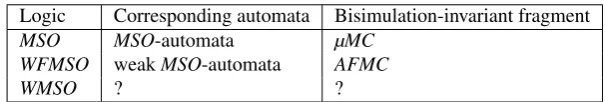
In this thesis we study the expressive power of variants of monadic second-order logic (MSO) on infinite trees by means of automata. In particular we are interested in weakMSOand well-foundedMSO, where the second-order quantifiers range respectively over finite sets and over subsets of well-founded trees. On finitely branching trees, weak and well-foundedMSOhave the same expressive power and are both strictly weaker than

MSO. The associated class of automata (called weakMSO-automata) is a restriction of the class characterizing

MSO-expressivity.

We show that, on trees with arbitrary branching degree, weakMSO-automata characterize the expressive power of well-foundedMSO, which turns out to be incomparable with weakMSO. Indeed, in this generalized setting, weakMSOgives an account of properties of the ‘horizontal dimension’ of trees, which cannot be described by means ofMSOor well-foundedMSOformulae.

In analogy with the result of Janin and Walukiewicz forMSOand the modalµ-calculus, this raises the issue of which modal logic captures the bisimulation-invariant fragment of well-foundedMSOand weakMSO. We show that the alternation-free fragment of the modalµ-calculus and the bisimulation-invariant fragment of well-founded

(4)

Introduction

Monadic second-order logic (MSO) is an expressive specification language in which first-order logic is extended with quantification over sets. By adding a successor relationRto the language, path quantification, reachability and other properties of transition systems can be described inMSO. We are interested in a particular kind of transition system, namely trees without leaves. In the sequel, we use the nametreeto refer to such infinite structures.

In the 60’s, Rabin [27] proved the decidability ofMSOon binary trees. This landmark result was obtained by an automata-theoretic characterization of the expressive power ofMSOon these structures. The idea is to define a class of automataCsuch that, for each formulaϕ∈MSO, we can construct an automatonAϕinCaccepting exactly the binary trees in whichϕis true. Viceversa, for each automatonAinCwe can find a formulaϕ_A∈MSOthat is true exactly in the binary trees that are accepted byA.

Rabin’s work became of direct interest for computer scientists one decade later, when it was realized that (infinite) trees can be used as models of the behavior of nonterminating systems [26]. In this framework,MSO

plays the role of an assembly-like language into which most specification languages (such as temporal logics and the modalµ-calculus) can be compiled [6] [10]. The underlying automata theory associated withMSOhas been developed consequently, extending Rabin’s characterization result to more general classes of structures.

In the 90’s, the work of Walukiewicz [33] [32] has provided a very general framework for investigatingMSO

by means of automata. In particular, in [33] a class of automata was introduced, which captures the expressive power ofMSOon trees with arbitrary (also infinite) branching degree. We will present them under the name of

MSO-automata.

Parallel to these developments, variants ofMSOhave also received attention. Among them,weak monadic

second-order logic(WMSO) is a quite appealing specification language, being computationally more manageable

thanMSO[21], but as expressive asMSOon simple structures such as streams [19]. Syntax and semantics of

WMSOare defined as forMSO, but for second-order quantifiers, which are restricted to range over finite sets only. An automata characterization ofWMSOon binary trees has been proposed by Rabin [28], to show thatWMSO

is strictly less expressive thanMSOon this class of structures. Automata forWMSOon binary trees have been further investigated in the ’80s by Muller, Saoudi and Schupp [24], introducing the notion ofweak alternating tree

automaton.

On structures that are more general than binary trees, automata theory forWMSOis less settled. It is a folklore result that weak alternating tree automata can be suitably generalized to serve as a characterization of the expressive power ofWMSOon finitely branching trees. We callweak MSO-automatathe resulting class of automata, being essentiallyMSO-automata where further constraints have been imposed on the structure of each run. This automata characterization leads to the result thatWMSOis weaker thanMSOalso on finitely branching trees.

In this thesis, we consider the question of howMSOandWMSOrelate on a more general class of structures, namely trees of arbitrary branching degree. The motivation is given by a simple observation onMSO-automata, namely that they are not able to distinguish between trees with finite or infinite branching degree. ThisFinite

Branching Propertycan be rephrased on the side of logic, by saying that eachMSO-formula that is true in some

tree is true in a finitely branching tree. As a consequence of that, the landscape of connections betweenMSOand

WMSOon arbitrarily branching trees radically changes with respect to the case of finitely branching trees.

• We can define aWMSO-formula that is only true in trees that are not finitely branching, meaning thatWMSO

does not have the Finite Branching Property. It follows thatWMSOis no more weaker thanMSOon trees of arbitrary branching degree, but the two logics haveincomparableexpressive power.

• On the side of automata, weakMSO-automata happen to have the Finite Branching Property, being a restricted version ofMSO-automata. It follows that, contrary to the case of finitely branching trees, weak

MSO-automata cannot serve as a characterization ofWMSOon the more general class of structures.

The outcome of this analysis is that the setting of finitely branching trees does not give the complete picture of

(7)

thesis we will be mainly interested in investigating the second question, that is, the theory of weakMSO-automata on trees of arbitrary branching degree. The structure of our work can be outlined as follows.

• After preliminaries, in the second chapter we rephrase Walukiewicz’s automata characterization ofMSOon arbitrarily branching trees. Given a formulaϕ∈MSO, we show how anMSO-automaton equivalent toϕcan be constructed, by induction on its syntactic shape. The flexibility ofMSO-automata makes relatively easy to prove that the tree languages that they recognize are closed under union and complementation. The hard part is to show that they are closed under projection, corresponding to the case in whichϕis of the form∃p.ψ, withpa set-variable. For this purpose, we emphasize the role of the Simulation Theorem, which provides a normal form forMSO-automata. The construction which is involved in this result turns out to be an useful benchmark to understand the nature ofMSO-expressivity.

• The third chapter considers the case of weakMSO-automata, defined as a restricted version of the automata introduced in the previous chapter. IfMSO-automata are tailored to serve as a characterization ofMSO, now we proceed in the converse direction, tailoring a logic that corresponds to weakMSO-automata. This is given as a variant ofMSO, which we callwell-founded monadic second-order logic (WFMSO). It is defined asMSObut for the semantics of second-order quantifiers, that are restricted to range over subsets of well-founded trees only. Analogously to the case ofMSO, given a formulaϕ∈WFMSO, we show by induction how a weakMSO-automaton equivalent toϕcan be constructed. Once again, the conceptual core of our argument is the case in whichϕis of the form∃p.ψ, withpa set-variable. By definition ofWFMSO, the variablepdoes not range over arbitrary sets of nodes, but only on the subsets of well-founded trees. To obtain the characterization result, we provide a normal form theorem for weakMSO-automata, which is the ‘weak’ counterpart of the Simulation Theorem, now tailored to the case ofWFMSO-quantification.

• In the fourth chapter we complete the correspondence between weakMSO-automata and WFMSO, by showing that each weakMSO-automaton is equivalent to some formulaϕ∈WFMSO. The proof of this result passes through the introduction ofnon-deterministic Büchi automata(NDBautomata), which are somehow intermediate between weakMSO-automata andMSO-automata. We prove that for each tree languageL, if bothLand its complement are recognized byNDBautomata, thenLis defined by someWFMSO-formula. This provides another automata characterization forWFMSO, in terms ofNDBautomata. Just as for the case of weakMSO-automata, alsoNDBautomata have a counterpart working on binary trees, which has been introduced by Rabin to characterizeWMSOon this restricted class of structures [28].

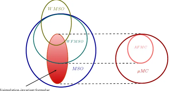
• The fifth chapter brings together all the work we did in the previous part to compare the expressive power

ofMSO,WMSOandWFMSOon different classes of structures. We argue that automata do not just give

an account of these logics, but also reveal which kind of specifications is better expressed by one logic with respect to the others. For instance, we observe thatMSOis stronger than WFMSOandWMSOin expressing properties of thevertical dimensionof trees, such as ‘each path has only finitely many nodes whose label includesp’. On the other hand,WMSOturns out to be more expressive thanMSOandWFMSO

on thehorizontal dimensionof trees, expressing properties such as ‘being finitely branching’. This latter property in particular cannot be expressed by means ofMSOorWFMSOformulae, as revealed by a careful analysis of the automata characterization provided for these two logics in the previous chapters. On the base of these observations, we state that, on arbitrarily branching trees,WFMSOandWMSOare respectively strictly weaker and incomparable withMSO. Next, we examine the question of howWFMSOandWMSO

are related. Despite of the fact that they are the same logic on finitely branching trees, we show that they are incomparable on trees of arbitrary branching degree. This is in some sense a refinement of the incomparability result forMSOandWMSO,WFMSObeing weaker thanMSO. In particular, it will follow as a corollary of another characterization result, which we consider one of the main contributions of this thesis: the bisimulation-invariant fragment ofWFMSOis as expressive as the alternation-free fragment of the modal

µ-calculus.

(8)

Chapter 1

Preliminaries

In this section we introduce some of the preliminaries and fix the notation. We refer to [17], [13] and [5] respectively for the terminology of Set Theory, Model Theory and Order Theory.

1.1 Sets, Functions and Relations

Sets are usually indicated with capital Latin lettersX,Y,Z, relations with capital Latin lettersR,Qand functions with small Latin letters f,gandh.

Sets LetXbe a set. We indicate with℘(X)the set of subsets ofX. For any subsetY⊆XofX, we denote with

X∖Y the set{x∈X∣x/∈Y}. IfY is afinitesubset ofX then we writeY⊆ωX. IfY isstrictly includedinX, meaning thatX∖Y is non-empty, we writeY⊊X. Given a setZ, we indicate withX×ZandX⊎Zrespectively the cartesian product and the disjoint union ofXandZ. For the setX×Zwe have the usual projection functionsπ1∶X×Z→X andπ2∶X×Z→Z.

Functions The notation f∶X→Ymeans that f is a function with domainXand codomainY. We refer toX→Y

as thetypeof f. The domain and codomain of f are also indicated respectively asDom(f)andCod(f). For any subsetZ⊆X, the set f[Z]is defined as{y∈Y ∣ f(x) =yfor somex∈Z}and we indicate with f↾Z∶Z→Y the

restriction of the function f toZ. The image f[X]off on the whole domainXis also denoted withRan(f). For any singleton set{z}, we indicate with f[z↦y]the function with domainX∪ {z}(wherezmay be inX) and codomainY, which is given by

f[z↦y](x) ∶= { y Ifx=z, f(x) Otherwise.

We say that f is1-1if f(x) =f(y)implies thatx=y, for allx,y∈X. We say that f isontoifRan(f) =Y. The function f∶X→Y isbijectiveif it is both 1-1 and onto. If f is 1-1, theinverseof f is the function f−1∶Ran(f) →X

assigning to eachy∈Ran(f)the uniquex∈X such thaty= f(x). Given functionsg∶X→Y andh∶Y →Z, we denote ash○g∶X→Z the composition ofgandh. Given functions f ∶X→Y and f′∶X′→Y′, we say that f′

extends f ifXandY are subsets respectively ofX′andY′, andf is equal to f_↾′_X. Functions are always assumed

total when not specified otherwise.

Relations LetX andY be sets. Given a binary relationR⊆X×Y, we defineDom(R) ∶= {π1(x,y) ∣ (x,y) ∈R} andRan(R) ∶= {π2(x,y) ∣ (x,y) ∈R}. For any elementx∈X, we indicate withR[x]the set{y∈Y ∣ (x,y) ∈R}. The relationsR+andR⋆are defined respectively as the transitive closure ofRand the reflexive and transitive closure of

R.

Natural Numbers The cardinality of a setXis indicated with∣X∣. Following von Neumann’s convention, we denote withωthe set of natural numbers with the usual order≤and we identify each natural numberi<ωwith the

set{0,1,2, . . . ,i−1}. For any finite subsetY ofω, we denote withMax(Y)andMin(Y)respectively the largest

and the smallest number occurring inY. A function f whose domain isγfor someγ≤ωand whose codomain is a setZis called asequence in Z. The standard notation forRan(f)is(zi)i_<γ, whereziindicates thatf(i) =z, for

(9)

⪯ifzi⪯zi+1for eachi<γ. In some contexts we refer to an infinite sequence(zi)i<ωof elements ofZas aZ−stream. We denote withZω_{the set of all}_Z−_streams.

1.2 Trees

Convention 1.1. Throughout this thesis we letPbe a fixed set ofpropositional letters, whose elements are denoted with small Latin letters p,qandr. We denote withCthe set℘(P)oflabelsonP. An element ofCis usually

indicated with the letterc. ◂

Definition 1.2(Labeled Transition System). AC-labeled transition systemis a tupleS= ⟨T,R,V⟩, whereT is a

set,R∶T×T is a binary relation andV∶P→ ℘(T)is a function. We say thatT is thecarrier,Ris thesuccessor relationandV is thevaluation functionof_S. For any pair(s,t) ∈Rwe say thatsis apredecessoroftandtis a

successorofs. For any pair(s,t) ∈R+, we say thatsis anancestoroftandtis adescendantofs. ⊲

We introduce trees as a particular kind of transitions systems.

Definition 1.3(Tree). A tupleT= ⟨T,sI,R,V⟩is aC-labeled treeifT= ⟨T,R,V⟩is aC-labeled transition system,

sI∈T is a distinguished point that has no predecessor, eachs∈T that is different fromsIhas a unique predecessor

and the following identity holds.

T = R⋆[sI]

The elements ofTare callednodesandsIis called therootofT. ⊲

Subtree Let_T= ⟨T,sI,R,V⟩be aC-labeled tree. AC-labeled treeT′= ⟨T′,s′I,R′,V′⟩is asubtreeofTifT′⊆T,

R′=R∩(T′×T′)andV′(p) =V(p)∩T′for eachp∈P. Observe that each subtree of_Tis uniquely determined by its carrier. Each nodes∈T uniquely defines a subtree of_Twith carrierR⋆[s]and roots, which we denote with_T.s.

Height and Leaf Theheightof a nodes∈T is inductively defined as follows: the root is the unique node at height 0; ifs∈T is a node of heighti, then eacht∈R[s]is a node of heighti+1. Two nodess,t∈T aresiblings

if there is a noder∈T such thats∈R[r]andt∈R[r]. Aleaf ofTis a nodes∈T such thatR[s] = ∅. A treeTis

leaflessif no node inTis a leaf.

Path and Branch LetS⊆T be a set of nodes. We say thatSis apathifS= (si)i_<kfor some sequence(si)i<k

withk≤ωandsiRsi+1for eachi<k. We say thatSisbackwards closedift∈SandsRtimpliess∈S, for alls,t∈T. Similarly,Sisfrontwards closedif, for alls∈SwithR[s] ≠ ∅, there is somet∈SwithsRt. The setSis abranchof

Tif it is a path and it is both frontwards and backwards closed.

Branching Degree With the terminologybranching degreewe refer to the cardinality of the setR[s]for nodes

s∈T. A tree_Tisfinitely branchingifR[s]is finite for alls∈T. For anyk<ω, we say that_Tis ak-bounded treeif

∣R[s]∣ ≤kfor alls∈T. In the specific case in which∣R[s]∣ =2 for alls∈T, we say thatTis abinary tree. We say

thatTisarbitrarily branchingif there is no special requirement on its branching degree.

Well-foundedness The treeTiswell-foundedif every path inTis finite. We denote withWF(T)the set of

well-founded subtrees ofT. A set of nodesS⊆Tiswell-closedifS⊆S′, whereS′is the carrier of some well-founded

subtree ofT. We use the notationWC(T)to indicate the set of well-closed subsets ofT.

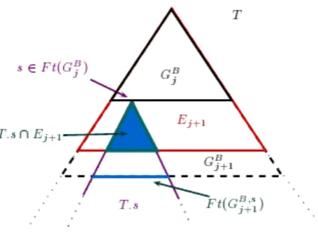
Frontier and Prefix We say thatGis afrontierofTifG∩Eis a singleton for every branchEofT. A setSis

aprefixofTif there exists a frontierGofTsuch thatS= {s∈T ∣sR⋆tfor somet∈G}. Observe that each prefix

SofTis the carrier of a well-founded backwards closed subtree ofT, with the property that for each nodes∈S

either none or all successors ofsare inS. It is easy to see that every prefix is uniquely determined by a frontier and viceversa. IfSis a prefix, we denote withFt(S)the associated frontier. Given two frontiersG1andG2ofT,

(10)

[image:10.595.165.430.74.243.2]

Figure 1.1: naming of parts.

p-variant Let p be a propositional letter (not necessarily in P). GivenT= ⟨T,sI,R,V⟩, suppose that Tp=

⟨T,sI,R,Vp⟩is a℘(P∪{p})-labeled tree such thatVp∶P∪{p} → ℘(T)is given asV[p↦S]for someS∈ ℘(T).

We refer to_Tpas ap-variantof_T. Ap-variant_Tpof_Tiswell-closedifVp(p) ∈WC(T). Similarly,_Tpis afinite p-variant ifVp(p) ⊆ωT. For a given setS∈ ℘(T), we denote withT[p↦S]thep-variantTp= ⟨T,sI,R,Vp⟩ofT

obtained by puttingVp=V[p↦S].

Remark 1.4(Coalgebraic Presentation [31]). It will be convenient to introduce an alternative presentation of trees, where the evaluation function and the successor relation are specified from the ‘local’ point of view of a node. Given aC-labeled treeT= ⟨T,sI,V,R⟩, we can representV∶P→ ℘(T)as alabeling functionσC∶T→Cand

R⊆T×T as asuccessor functionσR∶T → ℘(T). Given a nodes∈T, we callσC(s)thelabelofsand for each

p∈σC(s)we say thatsislabeled with p. SinceσCandσRhave the same domain, we can encode them as a single

functionσ∶T→ ℘(T)×C, assigning to each node the set of its successors and its label. Then we can representTas

a tuple⟨T,sI,σ⟩. Throughout this thesis we will mainly use this presentation for trees. ◂

Bisimulation is a notion of behavioral equivalence between processes [3]. Roughly, two processes are bisimilar when their behavior is indistinguishable from the point of view of an external observer. Transition systems are a mathematical model for processes and bisimulation is usually rendered as a binary relation. In the sequel we define this notion for the case of trees.

Definition 1.5(Bisimulation). GivenC-labeled treesT= ⟨T,sI,σ⟩andT′= ⟨T′,s′I,σ′⟩, abisimulationis a relation

Z⊆T×T′such that for all(t,t′) ∈Zthe following holds:

• σC(t) =σ′C(t′);

• for alls∈σR(t)there iss′∈σR(′ t′)such that(s,s′) ∈Z;

• for alls′∈σ′R(t′)there iss∈σR(t)such that(s,s′) ∈Z.

The treesTandT′arebisimilarif there is a bisimulationZ⊆T×T′including(sI,s′I). We writeT⇄T′to

indicate thatTandT′are bisimilar. ⊲

Given a treeT, theω-expansionTωofTis a canonical instance of a tree which is bisimilar toT. Intuitively,

Tωis given as a tree with the same root ofTandωcopies of any other nodes∈T.

Definition 1.6(ω-expansion). Given aC-labeled treesT= ⟨T,sI,σ⟩, theω-expansionofTis aC-labeled tree Tω= ⟨Tω,(sI,0),σω⟩defined as follows.

• The carrierTωis given as((T∖{sI})×ω)∪{(sI,0)}.

• For each node(s,i) ∈Tω, the labelσCω(s,i)of(s,i)is justσC(s), and the setσωR(s,i)of its successors is given

(11)

Remark 1.7. EachC-labeled treeT is bisimilar to itsω-expansionTω. A bisimulation relation Z⊆T×Tω witnessing this fact can be defined by putting

Z ∶= {(s,(s,i)) ∣s∈ (T∖{sI})andi<ω}∪{(sI,(sI,0))}.

In words,Zlinks each nodes∈T to all the copies ofsin theω-expansion. ◂

Convention 1.8. Throughout this thesis, every treeTthat we consider isleaflessandC-labeledif not specified

otherwise. ◂

1.3 Monadic Second-Order Logics on Trees

Definition 1.9(Syntax). Themonadic second-order languageonPis defined by the grammar

ϕ ∶∶= p⊑q∣R(p,q) ∣ ¬ϕ∣ϕ∨ϕ∣ ∃p.ϕ, (1.1)

where pandqare letters fromP. Given a formulaϕof the monadic second-order language, we denote with

FV(ϕ)andBV(ϕ)respectively the set offreeandboundletters occurring inϕ, defined as expected. We also adopt the standard convention that no letter occurs both free and bound inϕ, that is,FV(ϕ)andBV(ϕ)are disjoint.

The language ofmonadic second-order logic(MSOP),weak monadic second-order logic(WMSOP) and

well-founded monadic second-order logic(WFMSOP) is the monadic second-order language onP. We omit the subscript

Pwhen this is clear from the context. ⊲

Definition 1.10(Semantics). LetT = ⟨T,sI,V,R⟩be aC-labeled tree andϕa formula of the monadic second-order language onP. The semantics ofMSOis given by the following clauses, defining a truth relation⊧betweenTand

ϕ, by induction onϕ. IfT⊧ ϕholds, then we say thatϕistrueinT. T⊧ p⊑q iff V(p) ⊆V(q)

T⊧ R(p,q) iff for alls∈V(p)there is somet∈V(q)withsRt T⊧ ¬ϕ iff T/⊧ ϕ

T⊧ ϕ∨ψ iff T⊧ ϕorT⊧ ψ

T⊧ ∃p.ϕ iff there is ap-variantTpofTsuch thatTp⊧ ϕ

The semantics ofWMSOis given as the semantics ofMSObut for the clause of the existential quantifier, which is replaced by the following clause.

T⊧ ∃p.ϕ iff there is a finite p-variantTpofTsuch thatTp⊧ϕ

The semantics ofWFMSOis given as the semantics ofMSObut for the clause of the existential quantifier, which is replaced by the following clause.

T⊧ ∃p.ϕ iff there is a well-closedp-variantTpofTsuch thatTp⊧ϕ

Letϕ∈MSObe a formula. We denote with∥ϕ∥Pthe set ofC-labeled treesTsuch thatT⊧ϕ. The subscriptPis

omitted when the setPof propositional letters is clear from the context. ⊲

Remark 1.11. The monadic second-order language is aone-sortedlanguage: the only variables appearing are the letters from the setP, which are interpreted oversets. This definition is very convenient for the automata-theoretic perspective that we will consider throughout this thesis. Perhaps a different version of the monadic second-order language may have been expected, withtwosorts of variables. For instance, given a setVarof individual variables and the usual setPof set variables, consider the language defined by the following grammar.

ϕ ∶∶= x≈y∣x∈p∣xRy∣ ¬ϕ∣ϕ∨ϕ∣ ∃x.ϕ∣ ∃p.ϕ (1.2)

(12)

In fact the monadic second-order logics based on languages as in (1.1) or (1.2) are equivalent: the key observation is that an individual variablexcan be seen as a set variablepxwhose interpretation is restricted to

singletons. The translation from a formula as in (1.2) to a formula as in (1.1) crucially involves formulaeEmpty(p)

andSingl(p)defined by putting

Empty(p) ∶= ∀q(p⊑q)

Singl(p) ∶= (¬(Empty(p))))∧∀q(q⊑p→ (Empty(q)∨p⊑q)).

Either if we interpretEmpty(p)andSingl(p)according to the semantics ofMSO,WMSOorWFMSO, the formula

Empty(p)holds in a tree_TwhenV(p)is the empty set andSingl(p)whenV(p)is a singleton. We refer to [31],

remark 6.34 for more details on this translation. ◂

1.4 The Modal

µ

-Calculus

We refer to [31] for a thorough introduction to the modalµ-calculus (µMC).

Definition 1.12(Syntax). The language of the modalµ-calculus onPis given by the following grammar: ϕ ∶∶= p∣ ¬p∣ϕ∨ϕ∣ϕ∧ϕ∣ ◇ϕ∣ ◻ϕ∣µp.ϕ∣νp.ϕ,

wherepis a letter fromP, which does not occur under the scope of¬inµp.ϕandνp.ϕ. We callµandνrespectively

leastandgreatest fixpoint operator. Given a formulaϕ∈µMC, we define the setsFV(ϕ)andBV(ϕ)offreeand

boundvariables ofϕas expected, with fixpoint operators binding propositional letters analogously to quantifiers of

the monadic second-order language. We also adopt the standard convention thatFV(ϕ)andBV(ϕ)are disjoint.⊲

Definition 1.13(Semantics). Given a treeT = ⟨T,sI,V,R⟩, we inductively define themeaning∥ϕ∥Tof a formula ϕ∈µMCinTas follows.

∥p∥T ∶= _V(_p)

∥¬p∥T ∶= _T∖_V(_p)

∥ψ1∧ψ2∥T ∶= ∥ψ1∥T∩∥ψ2∥T

∥ψ1∨ψ2∥T ∶= ∥ψ1∥T∪∥ψ2∥T

∥◻ψ∥T ∶= {s∈T ∣ ∀t(sRt⇒t∈ ∥ψ∥T}

∥◇ψ∥T ∶= {s∈T ∣ ∃t(sRt∧t∈ ∥ψ∥T}

∥µp.ψ∥T ∶= ⋂{S⊆T ∣S⊇ ∥ψ∥T[p↦S]}

∥νp.ψ∥T ∶= ⋃{S⊆T ∣S⊆ ∥ψ∥T[p↦S]} We say thatϕistrueinT- notationT⊧ϕ- if the following condition holds.

T⊧ϕ iff sI∈ ∥ϕ∥T.

As for the case ofMSO, we denote with∥ϕ∥Pthe set ofC-labeled treesTsuch thatT⊧ϕ. The subscriptPis

omitted when the setPof propositional letters is clear from the context. ⊲

Formulae of the modalµ-calculus are classified according to theiralternation depth, which is informally given as the maximal length of a chain of nested alternating least and greatest fixpoint operators [4]. In particular, we are interested in thealternation-free fragmentof modalµ-calculus, which is the collection ofµMC-formulae without nesting of least and greatest fixpoint operators. The study of this fragment is motivated by computational feasibility, the alternation depth being the major factor in the complexity of model-checking algorithms for the modalµ-calculus [8].

Definition 1.14. We define the alternation-free fragment of modalµ-calculus (AFMC) as the set of formulae ϕ∈µMCwith the following property:

⋆ for any two subformulae ofϕof the formµp.ψ1andνq.ψ2, letterspandqdo not occur free respectively in

ψ2andψ1. ⊲

Example 1.15. The formulaµp.(◻p∨(νq.(◇q∧r)))is inAFMC, becausepdoes not occur free in◇q∧randq

does not occur free in◻p∨(νq.(◇q∧r)). Instead, the formulaµp.(νq.(◻p∨r∨◇q))is not inAFMCbecausep

(13)

1.5 Definability

Tree Languages We usually refer to a set ofC-labeled treesLas atree languageonP- or just as a tree language, ifPis clear from the context. We indicate withLthecomplementofL, i.e. the set ofC-labeled trees that are not in

L. A tree languageLisMSO-definableif there is a formulaϕ∈MSOsuch that∥ϕ∥ = L. We say thatϕdefinesL. GivenMSO-formulaeϕ1andϕ2, we say that they areequivalent- notationϕ1≡ϕ2- if∥ϕ1∥ = ∥ϕ2∥. We define in the same way analogous notions of definability forWMSO,WFMSO,µMCandAFMC.

Bisimulation Invariance The tree languageLisbisimulation closedifT⇄T′implies thatT∈ L ⇔T′∈ Lfor

each treeTandT′. A formulaϕ∈MSOisbisimulation invariantifT⇄T′implies thatT⊧ϕ⇔T′⊧ϕfor each treeTandT′. We define in the same way analogous notions of bisimulation invariance forWMSO,WFMSO,µMC

andAFMC.

Proposition 1.16. Each µMC-definable tree language is bisimulation closed.

Proposition 1.17(Janin-Walukiewicz Theorem [15]). The class of MSO-definable tree languages that are bisimu-lation closed coincides with the class of µMC-definable tree languages.

The following is a corollary of Bradfield’s result on the modalµ-calculus [4], showing that the alternation depth hierarchy does not collapse.

Proposition 1.18([4]). The class of AFMC-definable tree languages is strictly included in the class of µMC-definable tree languages.

1.6 Topological Complexity

We are interested in measuring the complexity of tree languages, from a topological point of view. In chapter 5 we are going to use the topological perspective to compare the expressive power of different logics on trees.

Borel Sets Given a topological space(X,τ), the classBorel(X) ⊆ ℘(X)ofBorel setsof(X,τ)is the smallest collection having all the open sets of(X,τ)as elements and that is closed under the set-theoretical operations of countable union and complementation. A subsetY⊆XisBorelif it is an element ofBorel(X).

Prefix Topology [9] We define a topology onC-labeled trees. For aC-labeled treeTand a natural numbern<ω thedepth-n prefixofT, denoted asT(n), is the subtree ofTwith carrier the prefix{s∈T ∣shas height at mostn}.

We say that two treesTandT′areequivalent up to height nifT(n)=T′(n). We call a setX of treesopenif, for

eachT∈ X, there is a natural numbern≥1 such that, for any treeT′, ifT(n)=T′(n)thenT′is inX. It can be

checked that this definition of open set yields a topology onC-labeled trees, which we callprefix topology.

The following results relate topological complexity and logical definability of tree languages.

Proposition 1.19([9]). LetLbe a tree language on P. IfLis WMSO-definable then it is a Borel set of the prefix topology.

Proposition 1.20([9]). The tree language on P defined by the formula µq.(◻q∨p)is not a Borel set of the prefix topology.

1.7 First-Order Logic

Throughout this section, we fix a finite setAof unary predicates. First, we present a first-order logic on signature given byA. It will be used later to define automata whose transition function is given in terms of first-order sentences.

Definition 1.21. LetVara set of first-order variables. We defineFor+(A)as the set of formulae generated by the following grammar.

ϕ,ψ ∶∶= ⊺ ∣ ∣x≈y∣x/≈y∣a(x) ∣ϕ∨ψ∣ϕ∧ψ∣ ∃x.ϕ∣ ∀x.ϕ (1.3)

The variablesxandyare from the setVar. Intuitively,For+(A)is the set of first-order formulae on signatureA, where unary predicates fromAcan only occur positively. Given a subsetSofA, we introduce the notation

τ+_S(x) ∶= ⋀

a∈S

(14)

The formulaτ+_S(x)is called apositive A-type. We use the convention that, ifSis the empty set, thenτ+_S(x)is⊺. Given a finite setX⊆ωFor+(A)of formulae,⋁Xis the formula given as the (finite) disjunction of all formulae in

X. Given a setY⊆For+(A)of formulae,SLatt(Y) = {⋁X ∣X⊆ωY}is the collection of all finite disjunctions of formulae inY. We indicate withFO+(A)the set ofsentencesfromFor+(A). ⊲

Definition 1.22(Semantics). Given a setX, a functionm∶A→ ℘(X)and a valuationv∶Var→X, we inductively define the notion of a formulaϕ∈For+(A)beingtruein(X,m,v)as follows.

(X,m,v) ⊧ ⊺

(X,m,v) /⊧

(X,m,v) ⊧ x≈y iff v(x) =v(y)

(X,m,v) ⊧ x/≈y iff v(x) ≠v(y)

(X,m,v) ⊧ a(x) iff x∈m(a)

(X,m,v) ⊧ ϕ∨ψ iff (X,m,v) ⊧ ϕor(X,m,v) ⊧ ψ

(X,m,v) ⊧ ϕ∧ψ iff (X,m,v) ⊧ ϕand(X,m,v) ⊧ ψ

(X,m,v) ⊧ ∃x.ϕ iff (X,m,v[x↦s]) ⊧ ϕfor somes∈X

(X,m,v) ⊧ ∀x.ϕ iff (X,m,v[x↦s]) ⊧ ϕfor alls∈X

The functionmis called amarking. We say that(X,m,v)is anA-structure. ⊲

GivenϕandψinFor+(A), in the sequel we freely use the notationϕ→ψto abbreviate¬ϕ∨ψ, provided that

¬ϕcan be rewritten into an equivalent formula inFor+(A).

Definition 1.23. For setsAandX, letMA,Xbe a set of markings of typeA→ ℘(X). We define a partial order⊴on MA,Xby putting

m⊴m′ iff m(a) ⊆m′(a)for alla∈A.

⊲

Letϕ∈FO+(A)be a sentence and(X,m,v)a first-order structure on signatureA. Sinceϕhas no free variables, we simply write(X,m) ⊧ϕto indicate thatϕis true in(X,m,v)for anyv. Each sentence inFO+(A)enjoys a monotonicity property that we introduce with the following remark.

Remark 1.24(Monotonicity). LetX be a set andϕ∈FO+(A)a sentence. We observe the following property ofϕ, that can be easily verified by induction onϕ:

⋆ Letm∶A→ ℘(X)be a marking such that(X,m) ⊧ϕ. For every markingm′∶A→ ℘(X)such thatm⊴m′we

have that(X,m′) ⊧ϕ. ◂

Definition 1.25(Basic Form). LetB1. . .BkandC1. . .Cjbe sequences of subsets ofA, possibly empty ifk=0 or

j=0. A sentenceϕ∈FO+(A)is inbasic formif it is of shape

ϕ = ∃x1. . .∃xk(diff(x¯)∧ ⋀

1≤i≤k

τ+_B_i(xi)∧∀z(diff(x¯,z) → ⋁

1≤l≤j

τ_C+

l(z))),

where eachτ+_B

i(xi)andτ

+

Cl(z)is a positiveA-type, as in definition 1.21, anddiff(y1, . . . ,yn) ∶= ⋀1≤m<m′<n(ym/≈ym′)

is aFor+(A)-formula stating that the interpretations ofy1, . . . ,ynare pairwise different. The sentenceϕis of the

form∃x1. . .∃xk(ψ1∧∀zψ2); we refer toψ1andψ2respectively as theexistentialand theuniversalpart ofϕ. We

indicate which positiveA-types appear in the sentence by saying thatϕdependson the sequenceB1. . .Bk,C1. . .Cj

of subsets ofA. We denote withBF+(A)the set of all sentences fromFO+(A)that are in basic form. ⊲

Using Ehrenfeucht-Fraïssé Games [13] it is possible to show that every sentenceϕ∈FO+(A)can be rewritten into an equivalent disjunction of sentences inBF+(A).

(15)

Remark 1.27. A sentenceϕ∈BF+(A)in basic form provides a quite informative picture of eachA-structure

(X,m)in which is true. By the particular shape ofϕ, the markingmhas the effect of partitioningXinto two sets

X_∃mandX_∀m=X∖X_∃m. The setX_∃mconsists of the witnesses for variablesx1, . . . ,xkin the existential part inϕ. By the

presence of the subformuladiff(x¯)inϕ, we know thatX_∃mcontainsexactly kelementss1, . . . ,sk. Foriwith 1≤i≤k,

the nodesi∈X_∃mis associated with the positiveA-typeτ+Bi(xi), meaning thatsi∈ ⋂a∈Bim(a). Analogously, the set

X_∀mcontains all the other elements ofX, which are witnesses for the variablezin the universal part ofϕ. We have thats∈ ⋂b∈Clm(b), for some positiveA-typeτ

+

Cl(z)occurring in the universal part ofϕ.

TheA-structure(X,m)is generally a ‘redundant’ representation of the sentenceϕ. Each elementt∈Xwitnesses some variableyofϕ, either in its existential or universal part, associated with a positiveA-typeτ+_S(y). This means that there is a setSt⊆A, such thatSis a subset ofStandtis in⋂a∈Stm(a). The key observation is thattwould still

be a ‘good’ witness for the variableyif we do not assign totany unary predicate inSt∖S. Following this intuition,

we say that a markingm♭∶A→ ℘(X)is ashrinkingofmif the following conditions hold. 1. Given anysi∈ {s1, . . . ,sk} =X_∃m,

{a∈A∣si∈m♭(a)} = Bi.

2. Given anyt∈X∖X_∃m=X_∀m,

{a∈A∣t∈m♭(a)} ⊆ {a∈A∣t∈m(a)}.

Furthermore,{a∈A∣t∈m♭(a)}is a minimal element of{C1, . . . ,Cj}with respect to the order⊆.

It is clear by the syntactic shape ofϕthat at least one shrinking ofmexists. Intuitively, the two conditions express that theA-structure(X,m♭)is a ‘non-redundant’ representation of the sentenceϕ, obtained by ‘contracting’ the representation(X,m). The markingm♭assigns to each elementtofXa subset ofA, which is⊆-minimal among the ones makingta witness for the corresponding variable inϕ, according to the partitionX_∃m∪X_∀m. These intuitions are fixed by the next three statements, which easily follow by the conditions onm♭expressed above.

a) m♭⊴m.

b) (X,m♭) ⊧ϕ.

c) For each marking ˜m∶A→ ℘(X), if ˜m⊴m♭and(X,m˜) ⊧ϕ, then ˜m=m♭. ◂

1.8 Game Terminology and Parity Games

Throughout this thesis we work with automata processing trees. A very convenient way to describe a run of such automata is by means of games. In particular, since all trees are assumed leafless, a run will generally be an infinite object, that we want to model through aninfinite game. For this purpose, we introduce some terminology and background on infinite games. All the games that we consider involve two players calledEloise(∃) andAbelard

(∀). In some contexts we refer to playerΠ, meaning that we want to specify a notion for a generic player in{∃,∀}.

Board Games Aboard gameGis a tuple(G∃,G∀,E,Win), whereG∃andG∀ are disjoint sets whose union

G=G_∃∪G_∀is calledboard,E⊆G×Gis a set ofedges, andWin⊆Gω_{is a set of}_G−_{streams. Each element}_u∈_G_is

aposition. Intuitively, ifuis an element ofGΠ, this means that playerΠis supposed to move from positionu. An

initialized board gameG@uIis a tuple(G∃,G∀,uI,E,Win)where(G∃,G∀,E,Win)is a board game anduI∈Gis

a distinguished position that we call theinitial positionof the game.

Matches Given a board gameG, amatchinGis a sequenceπ= (ui)i<αof positions ofG, whereαis eitherωor a natural number, and(ui,ui+1) ∈E for alliwithi+1<α. Analogously, given an initialized board gameG@uI,

we say thatπis a match inG@uI if it is a match inGandu0=uI. Ifα=ω, we say thatπis aninfinite match. Otherwise,α=kfor somek<ωandπis a finite match. We refer touk−1as thelastposition inπ, for which we use the notationlast(π). Sincelast(π)is an element ofG=G∃∪G_∀, then one of the two players, that we indicate with Π, is supposed to move fromlast(π). If there is nou∈Gsuch that(last(π),u) ∈E, we say that playerΠgets stuck inπ.

(16)

Strategies Given a board gameGand a playerΠ, letPMG_Π denote the set of partial matches ofGwhose last position belongs to playerΠ. Astrategy forΠis a function f of typePMG_Π→G. A matchπ= (ui)i_<αofG is

f -conformif for eachi<αsuch thatui∈GΠwe have thatui+1=f(u0, . . . ,ui). Given a partial matchπinDom(f), the position f(π)islegitimateif(last(π),f(π))is inE.

Givenu∈G, a strategy f∶PMG_Π→G, consider the following two conditions.

1. For each f-conform partial matchπofG@u, iflast(π)is inGΠthen f(π)is legitimate.

2. Eachf-conform total match ofG@uis won byΠ.

If f respects the first condition, we say that f is asurviving strategyforΠinG@u. Intuitively, if f is surviving then playerΠnever gets stuck in matches that are played according to f. Furthermore, if f respects both the first and the second condition, then we say that f is awinning strategyforΠinG@u. IfΠhas a winning strategy in

G@uthen we say thatuis awinning positionforΠinG. We denote withWinΠ(G)the set of positions ofGthat are winning forΠ.

Remark 1.28. As given above, a strategy for playerΠ is defined for allpartial matches inPMG_Π. However, throughout this thesis we will occasionally work with strategies which are only defined on a subsetXofPMG_Π. This is convenient for the purpose of merging several strategies f1,f2, . . . ,fktogether, obtaining a well-defined strategy

f′by the union of their graphs. In fact, we can assume that any partially defined strategy f∶X→Ghas domain

PMG_Π, by letting f(π)be an arbitrary position for all partial matchesπ∈PMG_Π∖X.

Similarly, notice that the property of a strategy f of being surviving or winning forΠonly depends on the value off on partial matches inPMG_Πthat are f-conform. By this observation, for the purpose of showing that f is surviving or winning, we usually define it just on f-conform partial matches inPMG_Π. ◂

Parity Games LetG = (G∃,G∀,E,Win)be a board game. Aparity mapis a functionΩ∶G→ωassigning a natural number to each position inG, such thatΩ[G]is finite. Given an infinite matchπ∈Gω_{, we denote with}

Inf(π)the set{k<ω∣Ω(u) =kfor infinitely manyu∈π}. Sinceπis infinite andΩ[G]is finite, thenInf(π)is non-empty. We say thatWinis aparity setif there exists a parity mapΩ∶G→ωsuch that

Win = {π∈Gω∣Min(Inf(π))is even}.

Aparity gameis a board gameG = (G∃,G∀,E,Win)whereWinis a parity set. We can see parity games as board

games whereWinpresents a quite regular structure. What makes them so appealing is that they enjoy a remarkable property which is calledpositional determinacy.

Positional Determinacy A strategyf∶PMG_Π→Gis calledpositionaliff(π) =f(π′)for eachπandπ′inDom(f) withlast(π) =last(π′). Intuitively, positional strategies only depend on the last position of partial matches on which they are defined. For this reason, a positional strategy with typePMG_Π→Gcan represented as a function of typeGΠ→G.

A board gameGwith boardGisdeterminedifG=Win_∃(G)∪Win_∀(G), that is, eachu∈Gis a winning position for one of the two players.

Theorem 1.29(Positional Determinacy of Parity Games, [7], [22]). For each parity gameG, there are positional strategies f_∃and f_∀respectively for player∃and∀, such that for every position u∈G there is a playerΠsuch that

fΠis a winning strategy forΠinG@u.

Following theorem 1.29, it will be convenient to assume that each strategy we work with in parity games is positional.

1.9 Stream Automata

Many of the concepts we presented so far are related to infinite sequences, also called streams. This motivates the introduction of automata operating on streams, that will be used in Chapter 2. We assume that the reader is already familiar with elementary notions of automata theory such as run and acceptance condition, for which we refer to [11].

Definition 1.30. AnX−stream automatonis a tupleZ= ⟨Z,zI,∆,Acc⟩whereZis a finite set of states,zI∈Zis an

initial state,∆∶Z×X→ ℘(Z)is a transition function andAcc⊆Zω_{is an acceptance condition. We say that}

Zis

deterministicif for each(z,x) ∈Z×X the set∆(z,x)is a singleton, andnon-deterministicotherwise. We callZa

(17)

For anX−stream(xi)i_<ω, arunρofZon(xi)i<ωis aZ−stream(zi)i<ωwherez0=zIandzi+1∈∆(zi,xi)for

eachi<ω. We say that(xi)i_<ωisacceptedbyZif there exists a runρofZon(xi)i<ωsuch thatρ∈Acc. We denote withL(Z)the set ofX−streams that are accepted byZ, also called thelanguageofZ. ⊲

Definition 1.31. For a setX, letL ⊆Xω_{be a set of}_X−_{streams. Similarly to the case of trees, we refer to}L_{as a}

stream language. We say thatLis anω-regular languageif there is anX−stream automaton_Zsuch thatL(Z) = L.

⊲

(18)

Chapter 2

Automata Characterization of

MSO

In this chapter we give an account of the expressive power ofMSOin terms of automata working on trees. For this purpose we introduceMSO-automata. The underlying idea is that, for each formulaϕ∈MSO, we can effectively construct anMSO-automatonAϕwhich isequivalenttoϕ, that is,Aϕhas the following property:

for any treeT,T⊧ϕ iff AϕacceptsT. (2.1)

2.1 MSO

-Automata: Definition

EveryMSO-automatonAwill be given as a tupleA= ⟨A,aI,∆,Ω⟩.

1. The first two components are a finite setAof states (also calledcarrier) and the initial stateaI∈AofA.

2. The automatonAdepends on an alphabet, which is standardly given as the setC∶= ℘(P), forPthe set of

propositional letters that we fixed with convention 1.1. The third component ofAis atransition function∆ of typeA×C→FO+(A). Operationally, this means that:

• the function∆takes as input a statea∈Aand the labelσC(s) ∈Cof a nodesofT;

• the function∆gives as output afirst-order sentence∆(a,σC(s)) ∈FO+(A)where statesa∈Aof the automaton can occur positively as unary predicates.

3. The fourth componentΩis a function of typeA→ω, assigning to each statea∈Aa natural numberΩ(a).

Before giving the formal definition ofMSO-automaton, we provide some intuitions on how the behavior ofAis

expressed in terms of∆andΩ. For this purpose we fix a treeT. The idea is to describe any run ofAonTin terms

of a game, which we call theacceptance gameofAonT. The acceptance game has two players: player∃claims

thatTshould be accepted byA, whereas player∀tries to refute this statement. Abasic positionof the game is a

pair(a,s) ∈A×T whereais a state of_Aandsis a node of_T. Amatchπproceeds in rounds, where each round is associated with a basic position. The interplay of the two players determines how we pass from a basic position

(ai,si)in roundito another basic position(ai+1,si+1)in roundi+1. Each round consists of two moves, that we can describe as follows.

• Move of∃:from position(ai,si) ∈A×T, player∃provides a marking m∶A→ ℘(σR(si))assigning sets of successors ofsito states ofA. Then(σR(si),m)is anA-structureaccording to definition 1.21.

Requirement:the markingmchosen by∃must be such that the sentence∆(ai,σC(si))istruein(σR(si),m). • Move of∀:given the markingm∶A→σR(si), player∀chooses the next basic position(ai+1,si+1) ∈A×T.

Requirement:the position(ai+1,si+1)chosen by∀must respectm, in the sense thatsi+1is inm(ai+1). Thereforeπconsists of basic positions - belonging to∃- and positions with markings - belonging to∀, which occur alternated.

π = (a1,s1),m1,(a2,s2),m2, . . . ,(an,sn),mn, . . .

We can assign a numeric value - which we callparity- to each position inπ. Each basic position(ai,si)

(19)

Observe that, ifπis infinite, then the minimum parity occurring infinitely often along the play is always associated with some basic position. The intuition is that positions with markings receive a conventional parity, which is not relevant for determining the winner of a match.

We are now ready to provide the formal definition ofMSO-automata.

Definition 2.1([33][31]). AnMSO-automatonon alphabetCis a tuple_A = ⟨A,aI,∆,Ω⟩where: • Ais a finite set of states;

• aI∈Ais theinitial stateofA;

• ∆∶A×C→FO+(A)is thetransition functionofA;

• Ω∶A→ωis theparity mapofA.

Given a treeT, theacceptance gameofAonT- notationA(A,T)- is a parity game defined according to the

rules of table 2.1. We recall that finite matches ofA(A,T)are lost by the player who gets stuck. An infinite match

ofA(A,T)is won by∃if and only if theminimumparity occurring infinitely often is even.

Position Player Admissible moves Parity

(a,s) ∈A×S ∃ {m∶A→ ℘(σR(s)) ∣ (σR(s),m) ⊧∆(a,σC(s))} Ω(a)

m∶A→ ℘(σR(s)) ∀ {(b,t) ∣t∈m(b)} Max(Ω[A])

Table 2.1: Acceptance game forMSO-automata

The treeTisacceptedbyAif and only if∃has a winning strategy inA(A,T)@(aI,sI). ⊲

Convention 2.2. In the sequel we assume that eachMSO-automaton is on alphabetC, if not specified otherwise.◂

Remark 2.3. A winning strategy f for∃inG = A(A,T)@(aI,sI)is in particular a surviving strategy for the

same player inG. Indeed, for each basic position(a,s) ∈A×T that is reached in some f-conform match ofG, the markingmsuggested by f makes∆(a,σC(s))true inσR(s), meaning that∃does not get stuck. The notion of surviving strategy can be conveniently restricted to subsets ofT. GivenW⊆T, we say that a strategy f′for∃in

Gissurviving in W if, for each basic position(a,s) ∈A×W that is reached in some f′-conform match ofG, the

markingmsuggested by f′makes∆(a,σC(s))true inσR(s). ◂

Remark 2.4. Given anMSO-automatonA= ⟨A,aI,∆,Ω⟩and a treeT, let fbe a strategy for∃inG = A(A,T)@(aI,sI).

SinceGis a parity game, we can assume f to bepositional. Therefore it can be represented as a function from basic positions (of f-conform matches ofG) to markings:

f ∶ (a,s) ↦ ma,s,

wherema,s∶A→ ℘(σR(s))is the move that f suggests to∃from position(a,s) ∈A×T. A very convenient way to

represent the information carried by f is by displaying its graph as a tree_T_f, defined as follows: • the carrierTf ofTf consists of the basic positions inDom(f);

• the root ofTf is the basic position(aI,sI);

• the successor functionσ_Rf∶Tf → ℘(Tf)is defined by putting

σ_Rf ∶ (a,s) ↦ {(b,t) ∣t∈ma,s(b)}

wherema,s= f(a,s).

• the labeling functionσ_Cf ∶Tf→Cis defined by putting

σ_Cf ∶ (a,s) ↦ σC(s)

(20)

An useful observation is that any f-conform partial matchπofA(A,T)corresponds to a unique pathBofTf,

and viceversa. In order to see that, observe thatBandπare both sequence of basic positions. The difference is that markings are represented explicitly inπas positions, whereas inBthey determine the successor relation between basic positions. However, both presentations have the same amount of information, namely which are the sets of admissible moves for∀along the play.

We refer toTf as thetree representationoff. It is convenient to fix aprojection functionπ₂f∶Tf→T, canonically

defined by puttingπ₂f∶ (a,s) ↦s. Observe thatπ₂fpreserves the tree structure, in the sense that, given basic positions

(a,s)and(b,t)inTf with(b,t)inσR(f a,s), the nodet=π2f(b,t)is inσR(s) =σR(π

f

2(a,s)). ◂

In the sequel we provide two basic examples of howMSO-automata andMSO-formulae can be associated, as described in (2.1).

Example 2.5. Letpandqbe letters inP. We want to provide anMSO-automatonAR(p,q)such that for any treeT

AR(p,q)acceptsT iff T⊧R(p,q).

LetAR(p,q)= ⟨A,aI,∆,Ω⟩be defined as follows.

A ∶= {a0,a1}

aI ∶= a0

∆(a0,c) ∶= { ∃

x(a1(x)∧∀y(y≠x→a0(y))) Ifp∈c

∀x(a0(x)) Otherwise

∆(a1,c) ∶= ⎧⎪⎪⎪⎨⎪⎪⎪

⎩

Ifq/∈c

∃x(a1(x)∧∀y(y≠x→a0(y))) Ifp∈candq∈c

∀x(a0(x)) Otherwise

Ω(a0) ∶= 0

Ω(a1) ∶= 0

LetTbe a tree. We provide an informal argument showing thatAR(p,q)acceptsTif and only if every node inT

labeled withphas a successor labeled withq.

The main observation is that, since both states ofAR(p,q)have parity even,∃is going to win all infinite matches

ofA(AR(p,q),T)@(aI,sI). Therefore the only chance that∀has to win is by letting∃get stuck. By definition of∆,

this happens if and only if the match arrives at some nodesthat is labeled withp, from which∃has to mark with

a1some nodet∈σR(s)such thatq/∈σC(t).

If a nodeswith this property exists, then∀has the power of bringing the match, in finitely many rounds, to a basic position of the form(a,s)for somea∈A. It suffices that at each round he selects the next basic position, of the form(b,t), in such a way thattR⋆s. If no nodeswith such property exists, the match is infinite and∃is the

winner. ◂

Example 2.6. Letpandqbe letters inP. We want to provide anMSO-automatonAp⊑qsuch that for any treeT

Ap⊑qacceptsT iff T⊧p⊑q.

The automatonAp⊑q= ⟨A,aI,∆,Ω⟩is defined as follows.

A ∶= {a0}

aI ∶= a0

∆(a0,c) ∶= { ∀

x a0(x) Ifq∈corp/∈c

Otherwise

Ω(a0) ∶= 0

Similarly to example 2.6 it is straightforward to check thatAp⊑qaccepts exactly the trees where every node labeled

(21)

2.2 Functional Strategies and Their Syntactic Characterization

The above examples give an idea of how first-order logic allows for rich and flexible specifications of the transition function of automata. As we will see in section 2.4, a remarkable consequence of thislogical perspective

is that closure properties of the tree languages definable byMSO-automata, such as union and complementation, are easily derivable from closure properties of the setFO+(A).

However, this flexibility is also a source of difficulties and complexity. In order to see that, letA= ⟨A,aI,∆,Ω⟩ be anMSO-automaton,_Ta tree andf a winning strategy for∃inG = A(_A,_T)@(aI,sI). Suppose that(a,s) ∈A×T

is a basic position occurring in an f-conform match ofG, with∆(a,σC(s)) ∈FO+(A)defined as∃x(a1(x)∧a2(x)) for somea1,a2∈A. In order to make this sentence true, the marking suggested by f must assign botha1anda2to the same nodet∈σR(s). This means that both position(a1,t)and(a2,t)can be chosen by∀to continue the match. Observe that∀’s move affects significantly the continuation of the match, because he does not only determine the next node -t, for instance - from which the match is played, but also the associated state - eithera1ora2.

It is convenient to visualize this situation by drawing thetree representationTf off, as in remark 2.4. If we

compareTf andTat the height of the setσR(s), we see thatTf is more ‘complex’ thanTwith respect tot: both

positions(a1,t)and(a2,t)are nodes ofTf. Intuitively, by the sole information that the nodetofTf is involved in

an f-conform match, we cannot determine which basic position is associated witht.

This ability of inferring the structure ofTf fromTis an essential ingredient of the projection construction

onMSO-automata, that we will introduce in section 2.4 as the automata counterpart of existential quantification inMSO. For this reason, we want to avoid the situation described above, by enforcing that each node in_Tis marked withat most onestate fromAalong f-conform matches ofG. This corresponds to the projection function

π₂f∶Tf →T being a1-1 correspondencebetweenTf andT. In fact, we can express the same condition in terms of

properties of the strategy f itself. For this purpose, we introduce the notion of a strategy for∃beingfunctional.

Definition 2.7. Let_A= ⟨A,aI,∆,Ω⟩be anMSO-automaton and_Ta tree. Letfbe a strategy for∃inA(_A,_T)@(aI,sI).

We say that f isfunctionalif, for each basic position(a,s) ∈Dom(f), the marking f(a,s)assigns to each node

t∈σR(s)at most onestateb∈A. ⊲

Our goal is to define a transformation, which allows to pass from an MSO-automaton Ato an equivalent

MSO-automatonA′such that, for each treeT, a winning strategy for∃inA(A′,T)@(aI,sI)can always assumed

to be functional. The idea is to tackle this question by providing asyntactic characterizationof functionality, in terms of the first-order sentences associated with the transition function ofMSO-automata.

For this purpose, we recall to the notion of sentence inbasic form, as in definition 1.25. By proposition 1.26, each sentence inFO+(A)is equivalent to a disjunction of sentences in basic form. It follows that the transition function∆ofAcan be assumed of typeA×C→SLatt(BF+(A))instead ofA×C→FO+(A). In the same spirit,

we want to show that the codomain of∆can be further restricted to first-order sentences having a quite specific syntactic shape, which will be associated with the property of a strategy for∃of being functional.

Definition 2.8(Functional basic form). Given a setAof unary predicates, letϕ∈BF+(A)be a sentence in basic form depending on sequencesB1. . .BkandC1. . .Cjof subsets ofA, that is,

ϕ = ∃x1. . .∃xk(diff(x¯)∧ ⋀

1≤i≤k

τ+Bi(xi)∧∀z(diff(x¯,z) → ⋁

1≤l≤j

τC+l(z))).

We say thatϕis infunctional basic formif eachSin{B1. . .Bk,C1. . .Cj}is either the empty set or a singleton. We denote withFBF+(A)the set of all sentences inBF+(A)which are in functional basic form. ⊲

Definition 2.9 (Non-deterministic automata). Let A= ⟨A,aI,∆,Ω⟩ be an MSO-automaton. We say thatA is

non-deterministicif∆has typeA×C→SLatt(FBF+(A)). ⊲

The following statement justifies the introduction of sentences in functional basic form as the ‘syntactic characterization’ of functional strategies for∃.

Proposition 2.10. LetA= ⟨A,aI,∆,Ω⟩be a non-deterministic MSO-automaton. Given any treeT, each surviving

strategy for∃inA(A,T)@(aI,sI)can be assumed to be functional.

The proof of proposition 2.10 requires some preliminary observation. In fact, it is not hard to imagine a surviving strategy f for∃inA(A,T)@(aI,sI)which isnotfunctional. Given a position(a,s) ∈A×T, suppose

thatm∶A→ ℘(σR(s))is a marking that makes∆(a,σC(s))true inσR(s). Since ∆(a,σC(s))is an element of

FO+(A), it enjoys themonotonicity propertydescribed in remark 1.24, meaning that each marking which extends

(22)

assigning more than one state to some node inσR(s). Then, f might suggests to∃the markingm′from position

(a,s), implying that it is not a functional strategy.

In order to show proposition 2.10, the key observation is that it is in∃’s interest to make the fewest number of moves available for∀. Thus a rational choice for her would be to assign to each node inσR(s)only the ‘strictly necessary’ amount of states that makes∆(a,σC(s))true. From this point of view,m′is not a very good suggestion for∃, because it generally assigns to each node more states than the markingm, which still makes∆(a,σC(s))true

inσR(s). By assuming that∃plays according to this idea of rationality, we can rule out redundant markings such asm′. Following these intuitions, we introduce the notion ofminimal strategy.

Definition 2.11. Let A= ⟨A,aI,∆,Ω⟩ be an MSO-automaton, T a tree and f a surviving strategy for ∃ in

A(A,T)@(aI,sI). Givena∈Aands∈T, consider the sentence∆(a,σC(s)), which we can assume to be an

element ofSLatt(BF+(A))by proposition 1.26. Given a disjunctϕ∈BF+(A)of∆(a,σC(s)), let us use the notation Ms,ϕfor the set

{m∶A→ ℘(σR(s)) ∣ (σR(s),m) ⊧ϕ}.

The setMs,ϕcan be ordered according to the relation⊴between markings, as given in definition 1.23. We say that

f isminimal forAandTif, for each basic position(a,s) ∈Dom(f), there is a disjunctϕof∆(a,σC(s))such that the marking f(a,s)is minimal with respect to the order⊴in the setMs,ϕ, that is, there is no markingm′∈ Ms,ϕ

such thatm′≠f(a,s)andm′⊴f(a,s). ⊲

Remark 2.12. Since we work with trees where a node can have infinitely many successors, the setMs,ϕ is generally infinite and we need some more arguing to show that it always has a minimal element with respect to the order⊴. The key observation is given by remark 1.27: a markingm∶A→ ℘(σR(s))that makesϕ∈BF+(A)true always has someshrinking. This means that there is a markingm♭∶A→ ℘(σR(s))such thatm♭is inMs,ϕ, we have thatm♭⊴m, and also there is no markingm′∈ Ms,ϕsuch thatm′≠m♭andm′⊴m♭. It follows in particular thatm♭

is a minimal element ofMs,ϕ. ◂

With the next proposition, we express the fact that∃can be always assumed to play according to the idea of rationality explained above.

Proposition 2.13. LetA= ⟨A,aI,∆,Ω⟩be an MSO-automaton andTa tree. The following are equivalent.

1. Player∃has a surviving strategy inA(A,T)@(aI,sI).

2. Player∃has a surviving strategy inA(A,T)@(aI,sI)which is minimal forAandT.

The same equivalence holds with ‘winning’ in place of ‘surviving’.

Proof We confine ourselves to the case of surviving strategies. It is immediate to check that the very same argument shows the statement also for the case of winning strategies. Direction(2⇒1)is immediate, so we focus on direction(1⇒2). Let f be a surviving strategy for∃inG = A(A,T)@(aI,sI). We want to define a strategy f♭

which is both minimal and surviving for∃inG. The definition of f♭is provided for each stage of the construction of a matchπ♭ofG, while maintaining an f-conform shadow matchπofG. For each roundzthat is played inπ♭ andπ, we want to keep the following condition.

The basic position occurring in the matchπ♭also occurs in the shadow matchπat the current round.

(‡)

The matchπ♭is initialized at position(aI,sI). We start the construction of the shadow matchπalso from position(aI,sI), so that condition(‡)holds for the first round. Observe that, since f is a surviving strategy for∃in G, thenπis indeed (the initial part of) an f-conform match.

Inductively, consider the case of some roundziwhere we are playing from the same basic position(a,s) ∈A×T

both inπandπ♭. Sinceπis f-conform, the strategy f suggests to ∃a markingm∶A→ ℘(σR(s))that makes ∆(a,σC(s))true. This means that there is some disjunctϕof∆(a,σC(s))that is true in(σR(s),m). By remark

2.12, there is also some markingm♭∶A→ ℘(σR(s))such thatm♭⊴mandm♭is a minimal element ofMs,ϕ. By definitionm♭makesϕtrue inσR(s), meaning that it also makes∆(a,σC(s))true inσR(s). Thereforem♭is a legitimate move for∃inπ♭and we let it be the suggestion of the strategy f♭.

(23)

the shadow matchπ. By letting∀choose position(b,t)inπ, we can keep the same basic position inπ♭andπat roundzi+1and condition(‡)is maintained for one more stage of the construction.

The strategy f♭that we just defined is minimal forAandT, according to definition 2.11. Moreover, in each

round that is played in the matchπ♭, the marking suggested by f♭is a legitimate move for∃, meaning that she never gets stuck inπ♭. Sinceπ♭has been constructed as an arbitraryf♭-conform match, this suffices to show that f♭

is a surviving strategy for∃. ◻

We are now ready to supply a proof of proposition 2.10.

Proof of proposition 2.10 LetA= ⟨A,aI,∆,Ω⟩be a non-deterministicMSO-automaton,Ta tree, and suppose that

∃has a surviving strategy f inA(A,T)@(aI,sI). By proposition 2.13 we can assume that f isminimal. Suppose

by way of contradiction that f is not functional. Let(a,s) ∈Dom(f)andt∈σR(s)be such that the marking

m = f(a,s)assigns two distinct statesa1,a2∈Atot. Since f is surviving and minimal then there is some disjunct ϕ∈FBF+(A)of∆(a,σC(s))such that(σR(s),m) ⊧ϕandmis minimal among the markings that makeϕtrue in σR(s).

Letm♭∶A→ ℘(σR(s))be some shrinking ofmas in remark 1.27. By definition,m♭⊴mand(σR(s),m♭) ⊧ϕ. By the particular syntactic shape ofϕ, the nodetwitnesses some variableyoccurring either in the existential or the universal part ofϕ, with associated positiveA-typeτ+_S(y). By definition,m♭assigns totexactly the states in the setS. Sinceϕis infunctionalbasic form, thenSis either empty or a singleton, meaning thattis inm♭(b)forat most one b∈A. Sincemassigns botha1anda2tot, it follows thatm♭≠m, contradicting the assumption thatmis minimal inMs,ϕ. Therefore f is a functional strategy and this completes the proof of the main statement. ◻

2.3 The Simulation Theorem

Our next goal is to show that everyMSO-automaton can be assumed to be non-deterministic. This statement, which is called theSimulation Theorem, can be considered the main technical result onMSO-automata.

Theorem 2.14(Simulation Theorem, [33]). Given an MSO-automatonA, there is an effectively constructible

non-deterministic MSO-automatonAP℘such that

A ≡ AP℘.

The transformation ofAinto a non-deterministic automatonAP℘is essentially performed in two steps.

1. FirstAis transformed into an equivalent non-deterministic automatonA℘ with a non-parity acceptance

condition.

2. ThenA℘is transformed into an equivalent non-deterministicMSO-automatonAP℘.

The conceptual core of the construction lies in the first step. As a side remark, notice that the automatonA℘is

not ‘officially’ anMSO-automaton, because of the non-parity acceptance condition. However, it makes sense to say that such automaton is non-deterministic, this property depending only on the type of the transition function. Before introducing further technical details, we gather some intuitions underlying the construction ofA℘. For the

purpose of giving the transition function ofA℘, a key observation is that each sentenceϕ∈BF+(A)can be seen as a sentence inFBF+(℘(A)), modulo a ‘change of base’ fromAto℘(A). To be more precise, suppose thatτ+_S(x)is a positiveA-type occurring inϕ, for some non-emptyS⊆A.

τ+_S(x) = ⋀

b∈S

b(x)

Now we may think ofτ+_S(x)as a℘(A)−type instead of anA-type.

τ+_S(x) = S(x)

Intuitively, what we did is to ‘encapsulate’ the conjunction intoS. The resulting formulaS(x)is a positive

(24)

Definition 2.15(Change of base). Fix a setAof unary predicates. Letϕ∈BF+(A)be a sentence in basic form depending on sequencesB1. . .BkandC1. . .Cjof subsets ofA. For each subsetSin the sequence, we define the

formulaτ℘_S(x)as follows:

τ℘_S(x) ∶= { S_⊺(x) IfS≠ ∅ Otherwise

We denote withϕ℘the sentence given as follows.

ϕ℘ = ∃x1. . .xk(diff(x¯)∧ ⋀

1≤i≤k

τ℘_B

i(xi)∧∀z(diff(x¯,z) → ⋁

1≤l≤j

τ_C℘

l(z)))

⊲

Note that, given ϕ∈BF+(A), the sentence ϕ℘ is in FBF+(℘(A)). Definition 2.15 provides the tools to characterize apowerset constructiononA. The idea would be to construct an automatonA♯with℘(A)as set

of states and a transition function∆♯∶ ℘(A) ×C→SLatt(FBF+(℘(A))), obtained from the transition function ∆∶A×C→FO+(A)ofAby using definition 2.15. The automatonA♯would be non-deterministic according to

definition 2.9.

This isalmostthe construction we are going to define. In fact we still need to specify the acceptance conditions ofA♯, in such a way that it is equivalent to the original automatonA. It turns out that the choice of℘(A)as carrier

is too coarse for this purpose.

In order to motivate this statement, letTbe a tree. The idea is that a matchπ♯ofA(A♯,T)represents a bundle

of matchesπ1, . . . ,πk ofA(A,T), which∃and∀play in parallel on the same branch ofT. We want to define

the winning conditions ofA(A♯,T)in such a way that∃winsπ♯if and only if she manages to win each match π1, . . . ,πk.

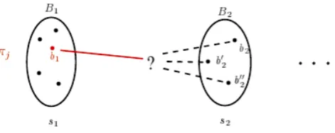
The problem is how to recover the structure of the various matchesπ1, . . . ,πkgiven the sole information ofπ♯.

Suppose that(B1,s1),(B2,s2), . . . ,(Bn,sn). . . are the basic positions visited alongπ♯, with(Bi,si)in℘(A)×T for

eachi<ω. Every matchπj∈ {π1, . . . ,πk}is associated with a sequence of basic positions(b1,s1),(b2,s2), . . . ,(bn,sn), . . .

such thatbiis inBifor eachi<ω. However, we do not knowwhich biis the element that we should pick inBito

[image:24.595.187.423.432.526.2]

recover the corresponding position ofπj: more than one choice is possible.

Figure 2.1: the problem of recovering the position ofπjwhich is associated with nodes2.

A possible way to deal with this problem is to assign atagto each statebi∈Bi, carrying the information of

which is the ‘precedent state’ ofAoccurring in the corresponding matchπj. For instance, ifbi∈Biandbi−1∈Bi−1 are such that(bi−1,si−1),(bi,si)are basic positions visited inπjat roundsi−1 andi, then we put the tagbi−1tobi.

This transformation turns every macro-stateB∈ ℘(A)into abinary relation R∈ ℘(A×A), where(b1,b2) ∈R stands for the stateb2∈Aequipped with tagb1∈A. The powerset construction onAmust be modified accordingly,

leading to arefined powerset constructiononA, which we denote withA℘.

Before the formal definition ofA℘, we need some preliminary work formalizing the intuitions given above. First, we introduce the notion oftrace. A sequence of positions(R1,s1),(R2,s2), . . . ,(Rn,sn). . ., with(Ri,si) ∈ (℘(A×A))×T, will induce a set of traces, indicating which matches ofAonTare associated with the sequence.

Definition 2.16([31]). LetAbe a finite set of states and letρ∈ (℘(A×A))ω_{be a}℘(_A×_A)−_stream.

ρ ∶= R0,R1, . . . ,Rn, . . .

Atraceα∈Aω_through

ρis anA−stream such thataiRi+1ai+1for alli<ω.

α ∶= a0,a1, . . . ,an, . . .

(25)

Definition 2.17([31]). LetAbe a finite set of states andΩ∶A→ωa parity map. We say that a traceα∈Aω_is_good if the minimum parity occurring infinitely often alongαis even, andbadotherwise. The setNBTΩ⊆ (℘(A×A))ω is defined as

NBTΩ ∶= {ρ∈ (℘(A×A))

ω_∣_{every trace through}

ρis good}.

⊲

The last component we need to consider before giving the formal definition of_A℘is the transition function. As we mentioned, the idea is to perform a ‘change of base’ on the transition function of the original automaton_A, passing from first-order sentences on signatureAto first-order sentences on signature℘(A). Now we need to shift the same argument to the signature℘(A×A), associated with the binary relations onAwhich will form the carrier ofA℘. For this purpose we introduce an intermediate step, transforming first-order sentences on signatureAinto

first-order sentences on signatureA×A.

Definition 2.18([31]). Let_A= ⟨A,aI,∆,Ω⟩be anMSO-automaton. Fixa∈Aandc∈C. The sentence∆⋆(a,c)is defined as

∆⋆(a,c) ∶= ∆(a,c)[(a,b)∖b∣b∈A],

where∆(a,c)[(a,b)∖b∣b∈A]denotes the sentence inFO+(A×A)obtained by replacing each occurrence of an

unary predicateb∈Ain∆(a,c)with the unary predicate(a,b) ∈A×A. ⊲

The next step is to put together definition 2.15 and 2.18 to characterize a transition function ranging over sentences on signature℘(A×A).

Definition 2.19. Let_A= ⟨A,aI,∆,Ω⟩be anMSO-automaton. Letc∈Cbe a label andR∈ ℘(A×A)a binary relation onA. By proposition 1.26 there is a sentenceΨ′_R_,_c∈SLatt(BF+(A×A))such that

⋀ a∈Ran(R)

∆⋆(a,c) ≡ Ψ′_R,c.

We defineΨR,cto be the sentence(ΨR′,c)℘, where the translation(−)℘is given as in definition 2.15. ⊲

Observe thatΨR,cis an element ofSLatt(FBF+(℘(A×A))). Now we have all the ingredients to provide the

definition of_A℘.

Definition 2.20. LetA= ⟨A,aI,∆,Ω⟩be anMSO-automaton. The automatonA℘ = ⟨A℘,a℘I,∆℘,Acc⟩is defined as

follows.

A℘ ∶= ℘(A×A) a℘_I ∶= {aI,aI}

∆℘(R,c) ∶= ΨR,c

Acc ∶= NBTΩ

HereΨR,cis given according to proposition 2.21 andNBTΩis given according to definition 2.17. The automaton

A℘is called therefined powerset construction onA. ⊲

The next step is to show that_A℘ is indeed equivalent to the original automaton_A. For this purpose, it is convenient first to prove two lemmata, associating the one-step behaviors of the automata_Aand_A℘.

Proposition 2.21. LetA= ⟨A,aI,∆,Ω⟩be an MSO-automaton andA℘ = ⟨A℘,a℘I,∆℘,Acc⟩its refined powerset

construction. Let R∈A℘be a binary relation,Ta tree and s a node ofT. Suppose that, for each a∈Ran(R), there

is a marking ma∶A→ ℘(σR(s))such that(σR(s),ma) ⊧∆(a,σC(s)). The following two statements hold.

1. There is a marking m⋆∶A×A→ ℘(σR(s))such that

a) (σR(s),m⋆) ⊧ ⋀a∈Ran(R)∆⋆(a,σC(s));

b) for each state a∈Ran(R), node t∈σR(s), state b∈A such that t∈m⋆(a,b), we have that t∈ma(b). 2. There is a marking m℘∶A℘→ ℘(σR(s))such that

MoL 2012 08: Expressiveness of Monadic Second Order Logics on Infinite Trees of Arbitrary Branching Degree

Expressiveness of Monadic Second-Order Logics

on Infinite Trees of Arbitrary Branching Degree

MSc Thesis

(Afstudeerscriptie)

Msc in Logic

Contents

Introduction

Chapter 1

Preliminaries

1.1

Sets, Functions and Relations

1.2

Trees

1.3

Monadic Second-Order Logics on Trees

1.4

The Modal

µ

-Calculus

1.5

Definability

1.6

Topological Complexity

1.7

First-Order Logic

1.8

Game Terminology and Parity Games

1.9

Stream Automata

Chapter 2

Automata Characterization of

MSO

2.1

MSO

-Automata: Definition

2.2

Functional Strategies and Their Syntactic Characterization

2.3

The Simulation Theorem