Dynamic Biological Functioning Important for Simulating
and Stabilizing Ocean Biogeochemistry
P. J. Buchanan1,2,3,4 , R. J. Matear2 , Z. Chase1 , S. J. Phipps1,4 , and N. L. Bindoff1,3,4
1Institute for Marine and Antarctic Studies, University of Tasmania, Hobart, Tasmania, Australia,2CSIRO Oceans and
Atmosphere, CSIRO Marine Laboratories, Hobart, Tasmania, Australia,3ARC Centre of Excellence in Climate System
Science, University of Tasmania, Hobart, Tasmania, Australia,4Antarctic Climate and Ecosystems Cooperative Research Centre, University of Tasmania, Hobart, Tasmania, Australia
Abstract
The biogeochemistry of the ocean exerts a strong influence on the climate by modulating atmospheric greenhouse gases. In turn, ocean biogeochemistry depends on numerous physical and biological processes that change over space and time. Accurately simulating these processes is fundamental for accurately simulating the ocean’s role within the climate. However, our simulation of these processes is often simplistic, despite a growing understanding of underlying biological dynamics. Here we explore how new parameterizations of biological processes affect simulated biogeochemical properties in a global ocean model. We combine 6 different physical realizations with 6 different biogeochemical parameterizations (36 unique ocean states). The biogeochemical parameterizations, all previouslypublished, aim to more accurately represent the response of ocean biology to changing physical conditions. We make three major findings. First, oxygen, carbon, alkalinity, and phosphate fields are more sensitive to changes in the ocean’s physical state. Only nitrate is more sensitive to changes in biological processes, and we suggest that assessment protocols for ocean biogeochemical models formally include the marine nitrogen cycle to assess their performance. Second, we show that dynamic variations in the production, remineralization, and stoichiometry of organic matter in response to changing environmental conditions benefit the simulation of ocean biogeochemistry. Third, dynamic biological functioning reduces the sensitivity of biogeochemical properties to physical change. Carbon and nitrogen inventories were 50% and 20% less sensitive to physical changes, respectively, in simulations that incorporated dynamic biological functioning. These results highlight the importance of a dynamic biology for ocean properties and climate.
Plain Language Summary
The ocean’s biogeochemistry is important for controlling concentrations of atmospheric greenhouse gases and therefore plays a key role in climate. An important part of ocean biogeochemistry are the numerous biological processes that occur in the ocean. In this study, we use a number of newly proposed ways to simulate the complex biological processes of the ocean. We find that these formulations provide a number of important improvements when combined. Not only do they allow the ocean model to simulate observed, regional features of ocean biology, but they also improve the simulation of ocean biogeochemistry on a global scale. We uniquely find through changing the biological and physical characteristics of the ocean that the nitrogen cycle is the most responsive to biological change, and we suggest that future assessments of ocean biogeochemical models use nitrate as a primary assessment tool. Finally, we find that including dynamic biological processes reduces the ocean’s sensitivity to physical changes. Ocean biology could therefore act as a buffer to the effects of climate change through its response to environmental conditions.1. Introduction
The ocean is a powerful player in the global climate system. Due to its large volume and surface area, the biogeochemical properties of the ocean are an important control on atmospheric concentrations of carbon dioxide and other greenhouse gases. The biological pump, which involves the fixation of carbon and other elements within organic matter and their subsequent transfer to depth, plays an important role in regulating atmospheric CO2. There is strong evidence from proxy and model studies that variations in the strength of the biological pump, in conjunction with reorganizations of ocean circulation, played a major role in setting past
RESEARCH ARTICLE
10.1002/2017GB005753
Key Points:
• Nitrate is highly sensitive to biogeochemical model parameterizations and useful for model assessment • Dynamic biological functioning
improves the simulated distribution of major biogeochemical fields in a global ocean model
• Dynamic biological functioning reduces the sensitivity of important fields, like carbon, to physical changes
Supporting Information: • Supporting Information S1
Correspondence to: P. J. Buchanan,
Citation:
Buchanan, P. J., Matear, R. J., Chase, Z., Phipps, S. J., & Bindoff, N. L. (2018). Dynamic biological functioning important for simulating and stabilizing ocean biogeochemistry. Global Biogeochemical
Cycles,32, 565–593.
https://doi.org/10.1002/2017GB005753
Received 29 JUN 2017 Accepted 14 FEB 2018
Accepted article online 21 FEB 2018 Published online 16 APR 2018
climates (Buchanan et al., 2016; Kohfeld et al., 2005; Schmittner & Somes, 2016). The response of the biological pump under anthropogenic climate change will influence the evolution of Earth’s climate.
Accurately simulating biological processes in the ocean is therefore fundamental for accurately simulating the behavior of the climate system over millennial time scales. In its broadest sense, the processes that govern the ocean’s biological pump can be defined as (1) those that create organic matter from inorganic matter, (2) those that create inorganic matter from organic matter (remineralization), and (3) those that control the quantities of elements involved in these exchanges. All three processes can be depicted simply by equation (1), originally given by Redfield (1963).
106CO2+16HNO3+H3PO4+122H2O<=>(CH2O)106(NH3)16(H3PO4) +138O2 (1)
Here production of organic matter involves the forward reaction, while the remineralization of organic matter involves the reverse reaction. The quantities of elements involved are found by balancing the chemical formula and coincide with the Redfield ratio of C:N:P:O2as 106:16:1:-138.
A few equations defined in seminal studies from the twentieth century are largely used in ocean biogeo-chemical models to simulate the biological pump. Nutrient and light availability are commonly used to limit the maximum potential growth rate set by temperature (Eppley, 1972). Typically, the nutrient requirements for phytoplankton growth are based on an unchanging Monod function (Dugdale, 1967; Monod & Wollman, 1947), such that a given phytoplankton type has fixed nutrient requirements. The remineralization of organic matter through the water column is commonly parameterized according to a function of depth, often referred to as a Martin curve (Martin et al., 1987), which again is typically fixed for a given phytoplankton type. Finally, the quantities of elements that are involved in the reaction of equation (1) are prescribed according to the Redfield ratio (Fleming, 1940; Redfield, 1963; Redfield et al., 1937), or a variation thereof (Anderson, 1995; Takahashi et al., 1985), and also remain unchanged.
These traditional equations, which are explained more completely in Appendix A, are a rudimentary rep-resentation of what is a complex ecological web with biogeochemical consequences (Worden et al., 2015). Modeling studies using the traditional equations (e.g., Buchanan et al., 2016; Joos, 1999; Mariotti et al., 2012; Matear & Hirst, 1999; Sarmiento et al., 1998; Schmittner, 2005; Schmittner & Somes, 2016) are thus com-promised by overly simplistic responses to physical changes. However, simulating the biological pump in a more realistic way is challenging, and the community has slowly integrated more complex ecosystem models and processes to improve the simulation of global ocean biogeochemistry (Aumont et al., 2017; Boyd & Doney, 2002; Dutkiewicz et al., 2013; Le Quéré et al., 2016; Weber & Deutsch, 2012). These studies have each demonstrated that simulated biogeochemical fields are improved by including additional biogeo-chemical complexity, but each has focussed on particular biogeobiogeo-chemical tracers of interest. Simulations that explore the role of the biological pump in a future climate using the current suite of ocean biogeochemi-cal models are therefore difficult to interpret because each represents biologibiogeochemi-cal processes in different ways, which may show divergent projections of key properties (see the multimodel analysis by Laufkötter et al., 2016, for an example).
particularly as certain biogeochemical tracers like oxygen and carbon appear to be highly sensitive to physical change (Cocco et al., 2013; Marinov et al., 2008; Séférian et al., 2013).
Fortunately, a number of simple parameterizations that mechanistically produce the large-scale features of marine biological communities have been designed for ease of uptake into ocean biogeochemical models. They are improvements on the traditional equations that add flexibility to the limitation of primary production by phosphate and nitrate (Smith et al., 2009), remineralization rates (Marsay et al., 2015; Weber et al., 2016), and stoichiometry (Galbraith & Martiny, 2015). We assess these new parameterizations and their effect on global ocean biogeochemical fields using the ocean component of the Commonwealth Scientific and Indus-trial Research Organisation Mark 3L (CSIRO Mk3L) Earth system model. In consideration of uncertainty in the physical state of the ocean, we make this assessment using a number of plausible preindustrial physical states and explore the influence of physical and biological processes on ocean biogeochemistry. We find that the dynamic biological functioning produced by these simple formulations in combination is fundamental for simulating and stabilizing ocean biogeochemistry.
2. Experimental Design
To assess the sensitivity of biogeochemical changes to variations in both the physical and biological state of the ocean, we generated six unique physical and biogeochemical model states. Physical states were gener-ated using the Ocean General Circulation Model (OGCM) from within the CSIRO Mk3L (Phipps et al., 2013). Biological states were generated by modifying the ocean biogeochemical model attached to the OGCM. A description of the ocean biogeochemical model is located in Appendix A. A total of 36 experiments were run for 10,000 years toward equilibrium for all physical and biogeochemical fields. In the following we detail how each unique physical and biological state was generated.
2.1. Physical States
Six physical states were generated by forcing the OGCM with six realizations of the preindustrial climate. The OGCM requires monthly climatologies of sea surface temperature (∘C), sea surface salinity (practical salinity unit), and surface wind stresses (Pa) to calculate surface fluxes and large-scale ocean dynamics. The biogeo-chemical model requires climatologies of sea ice cover, surface wind speeds, incident short wave radiation, and the aeolian deposition of iron and reactive nitrogen to the surface ocean. With the exception of the aeo-lian deposition fields, which were provided by Mahowald et al. (2005) for iron and Lamarque et al. (2013) for reactive nitrogen, each physical state was generated using a unique set of surface climatologies. The model interpolates linearly in time between the climatological means for each calendar month.
The preindustrial climatologies for the Mk3L physical state were provided by a 10,000 year spin up of the flux adjusted CSIRO Mk3L coupled climate system model. For the remaining five physical states, surface clima-tologies were provided by five climate system models from the Climate Model Intercomparison Project phase 5 (CMIP5) multimodel ensemble (Taylor et al., 2012). These models comprise GFDL-ESM2G, IPSL-CM5A-MR, HadGEM2-CC, MPI-ESM-MR, and MRI-CGCM3 (Table 1). As part of the CMIP5 protocol, these groups were required to undertake a multicentury control simulation under preindustrial conditions. The surface fields required to force the OGCM and biogeochemical model were downloaded from the Earth System Grid Federation database (https://esgf-node.jpl.nasa.gov/projects/esgf-jpl/), and the months over the final 10 years of the preindustrial run were averaged to provide monthly climatologies. These climatologies were regridded onto CSIRO Mk3L grid space using theFerretprogram.
Note that the incident shortwave radiation field for HadGEM2-CC was unavailable and was substituted by the net shortwave radiation field of GFDL-ESM2G, which a priori had the most similar sea surface temperature climatology to HadGEM2-CC with anr2of 0.98 and a mean bias of+0.01∘C.
All ocean physical states were therefore generated using the OGCM physics of CSIRO Mk3L but were forced by different surface boundary conditions. We will hereby refer to the six physical states according to the ori-gins of the boundary conditions by which they were forced: Mk3L, Geophysical Fluid Dynamics Laboratory (GFDL), Institut Pierre-Simon Laplace (IPSL), Hadley Centre Global Environmental Model (HadGEM), Max Planck Institute for Meteorology (MPI), and Meteorological Research Institute (MRI) ocean states.
2.2. Biological States
Table 1
A Summary of the Physical and Biological States That Were Produced Within the Ocean Biogeochemical Model
Physical states Modeling group Experiment Variables
1. Mk3L Commonwealth Scientific and Industrial Research Organisation (Phipps et al., 2013) tos, sos, rsntds, tauu, tauv, sfcWind, sic 2. GFDL NOAA Geophysical Fluid Dynamics Laboratory piControl tos, sos, rsntds, tauu, tauv, sfcWind, sic 3. IPSL Institut Pierre-Simon Laplace piControl tos, sos, rsntds, tauu, tauv, sfcWind, sic 4. HadGEM Met Office Hadley Centre piControl tos, sos, tauu, tauv, sfcWind, sic 5. MPI Max Planck Institute for Meteorology piControl tos, sos, rsntds, tauu, tauv, sfcWind, sic 6. MRI Meteorological Research Institute piControl tos, sos, rsntds, tauu, tauv, sfcWind, sic Biological states Function Modification dependencies Proposed by
1. Base None
2. OUK Nutrient limitation of phytoplankton NO3and PO4 (Smith et al., 2009) 3. RemT Depth of remineralization Temperature (Marsay et al., 2015) 4. RemP Depth of remineralization Picoplankton fraction of community (Weber et al., 2016) 5.Vele Elemental composition of organic matter NO3and PO4 (Galbraith & Martiny, 2015) 6. COM Combination of OUK, RemP, andVele as above
Note.Five of the six physical states were generated using surface climatologies produced by the preindustrial control (piControl) run as part of the Climate Model
Intercomparison Project phase 5 (CMIP5; Taylor et al., 2012). The surface climatologies used to force the OGCM of CSIRO Mk3L were sea surface temperature (tos), sea surface salinity (sos), surface downward eastward stress (tauu), and surface downward northward stress (tauv). Surface climatologies additionally needed for the biogeochemical model were net downward shortwave flux at sea water surface (rsntds), wind speed (sfcWind), and sea ice area fraction (sic). Each biological state was tested within each of the six physical states, for a total of 36 experiments.
recently proposed formulations that express how marine biology responds to its environment (Galbraith & Martiny, 2015; Marsay et al., 2015; Smith et al., 2009; Weber et al., 2016) (Table 1).
2.2.1. Basic Biogeochemical Model (Base)
TheBasebiogeochemical model used a number of equations defined in seminal studies from the twentieth century to simulate the processes that govern biological production, remineralization, and stoichiometry in the ocean, and these are described in more detail in Appendix A. The Base biological state ensured that the nutrient requirements for growth, the rate of remineralization, and the stoichiometry of organic matter were constant everywhere. The Base biological state therefore represented a biological community that did not alter its functioning in response to environmental change. In other words, the biogeochemical features of the phytoplankton community did not change.
2.2.2. Variable Nutrient Limitation of Organic Matter Production (Optimal Uptake Kinetics)
The universal application of Michaelis-Menten kinetics to nutrient uptake by phytoplankton is an oversim-plification (Flynn, 2003), and optimal uptake kinetics (OUK) was developed to express how phytoplank-ton optimize their nutrient uptake depending on ambient nutrient concentrations (Smith et al., 2009). Essentially, OUK captures how different phytoplankton communities respond and grow within different nutri-ent regimes. It assumes that phytoplankton dynamically alter their internal resources between surface uptake sites, which absorb external nutrients, and internal enzymes, which assimilate the nutrients for growth. By taking this phenomenon into account, Smith et al. (2009) were able to calculate faster growth rates of phy-toplankton in oligotrophic waters by assuming that these phyphy-toplankton directed more resources toward surface uptake sites.
To implement OUK within CSIRO Mk3L (experiment OUK), the fraction of the internal nutrient store that is allocated to either surface uptake sites (fA) or internal enzymes (1−fA) was calculated.
fA=max [(
1+ √
[NO3] 0.187
)−1
,
( 1+
√
[PO4]⋅N:P 0.187
)−1]
(2)
Smith et al. (2009). Once the partitioning of nutrient between internal stores (fA) was solved, the nutrient limitation terms for PO4and NO3were calculated
PO4OUK lim =
[PO4] [PO4]
1−fA + 0.187
fA⋅N:P
(3)
NO3OUK lim =
[NO3] [NO3]
1−fA +0.187
fA
(4)
and applied to the calculation of export production (equation (A5)).
It is important to note that the limitation term for iron (Felim) was not altered (equation (A4)). It was unchanged from its Michaelis-Menten formulation with a half-saturation constant (KFe) equal to 0.1μmol m−3. The limitation on growth caused by iron was therefore unchanged across the global ocean.
2.2.3. Temperature-Dependent Remineralization (RemT)
Since the Martin curve was proposed, numerous studies have questioned its application within different oceanic environments. Sediment trap measurements have shown large variations in the power law expo-nentb(Berelson, 2001; Francois et al., 2002), with values commonly ranging from−1.3to−0.6. These results have shown that generalizing a common rate of remineralization across the ocean is an oversimplification (Olli, 2015).
Temperature could be an important factor with primary control over the rate of remineralization within the ocean interior. The long-standing relationship between temperature and the growth rate of marine plank-ton (Eppley, 1972) also extends to heterotrophic bacteria in the ocean interior (Laws et al., 2000). Moreover, there appears to be no evidence for microbial community adaptation to latitudinal temperature differences (Bendtsen et al., 2015). If this is true, then cooler regions of the ocean should support reduced rates of rem-ineralization and therefore allow more organic matter to enter deeper waters (i.e., less negativebvalues), while warmer regions should have steeper remineralization profiles, where less organic matter enters deeper waters. Strong evidence for a temperature-dependent remineralization rate was demonstrated by Buesseler et al. (2007), who reported that roughly 50% of the organic matter falling from 150 m in subarctic waters was present at 500 m, while only 20% remained at 500 m in the subtropical North Pacific.
To apply a temperature-dependent remineralization rate within CSIRO Mk3L (experimentRemT), we altered
thebexponent of the Martin curve according to Marsay et al. (2015).
b= −(0.062⋅T+0.303) (5)
whereTis the average temperature (∘C) of the upper 500 m of the water column.
Marsay et al. (2015) predicted the flux of particulate organic matter into the ocean interior across four sites in the North Atlantic Ocean using this relationship. However, using equation 5 gave values greater than−0.4 across large areas of the high latitudes, as mesopelagic water temperatures are typically less than 2∘C. Consid-ering that estimates of thebexponent based on observations have rarely featured values greater than−0.6 (Berelson, 2001; Francois et al., 2002), we applied an upper limit of−0.6 to equation (5).
2.2.4. Phytoplankton-Dependent Remineralization (RemP)
Recently, Weber et al. (2016) found that the composition of the phytoplankton community, specifically the component fraction of picoplankton (Fpico), was a superior predictor of organic matter transfer into the ocean interior. Using global distributions of nutrient and oxygen tracers along transport pathways, rather than directly measuring organic flux, they found thatFpicocould explain 93% of the variance in the observations, while temperature could only explain 70%.
Here we used the equation provided by Weber et al. (2016) within CSIRO Mk3L (experimentRemP), where
the transfer efficiency (Teff) of organic matter from the bottom of the euphotic zone to 1,000 m was determined by
Because CSIRO Mk3L does not simulate picoplankton, we estimated Fpico for each surface grid using a linear parameterization, where high Fpico values are found in regions with low organic carbon produc-tion (Corg) and Cmax
org represents the maximum rate of organic carbon production from the ocean at the previous day.
Fpico=0.51−0.26⋅ Corg(mg C m −2h−1)
Cmax
org(mg C m−2h −1
) (7)
This simple parameterization is informed by the estimates ofFpicoreported by Weber et al. (2016), where val-ues of 0.3 were found in highly productive regions and valval-ues as high as 0.55 were found in the oligotrophic subtropical gyres. It is also informed by global observations of particle distributions, where picoplankton dominate low productivity regions and microplankton dominate the highly productive regions (Kostadinov et al., 2009). Furthermore, small taxa are observed to dominate Southern Ocean communities during non-bloom conditions (Deppeler & Davidson, 2017), leading to weak organic flux to depth (Ducklow et al., 2015; Weeding & Trull, 2014). A maximum production at the previous day sets Cmax
org, which allows for simi-lar values ofFpicobetween different ocean states, but alters the spatial patterns. This parameterization also returnedTeffvalues in the range provided by Weber et al. (2016) from 0.05 to 0.3 for subtropical and polar regions, respectively.
When theTeffwas known, we solved for thebexponent in the Martin curve using
b= log(Teff) log(1100,000)
=log(Teff)
1 (8)
where the depth of the euphotic zone was always 100 m, and the transfer efficiency of organic matter falling out of the euphotic zone is referenced to 1,000 m.
2.2.5. Variable Elemental Ratios (Vele)
While the Redfield ratio (Redfield et al., 1937) remains a cornerstone of our understanding of ocean bio-geochemistry, there is an increasing support for non-Redfield ratios. Numerous studies that together span the global ocean have reported wide variations in the C:N:P ratios of marine organic matter (supporting information Table S1; Anderson, 1995; Anderson & Sarmiento, 1994; Boulahdid & Minster, 1989; Fraga et al., 1998; Geider & La Roche, 2002; Hedges et al., 2002; Klausmeier et al., 2004; Martin et al., 1987, 2013; Peng & Broecker, 1987; Takahashi et al., 1985; Weber & Deutsch, 2010).
Observed variations in nitrogen and carbon stoichiometry (C:N:P ratios) are now considered to be strongly related to nutrient availability in the surface ocean. Higher C:P and N:P ratios are commonly observed in those regions prone to nutrient limitation, while nutrient-replete regions typically show much lower C:P and N:P ratios (Boulahdid & Minster, 1989; Galbraith & Martiny, 2015; Geider & La Roche, 2002; Klausmeier et al., 2004; Martiny et al., 2013). In an attempt to quantify this relationship, Galbraith and Martiny (2015) built a statisti-cal model to predict P:C and N:C ratios of organic matter across the ocean surface using only PO4and NO3 concentrations.
Using their empirical model, we calculated C:P and N:P ratios in CSIRO Mk3L (experimentVele):
C:P= (6.9⋅
[PO4] +6 1,000
)−1
(9)
N:C=0.125+ 0.03⋅[NO3] 0.32+ [NO3]
(10)
N:P=C:P⋅N:C (11)
The Redfield ratio estimates an Orem:P ratio of−138:1 and an Nden:P ratio of−94.4:1 by assuming that all organic matter is well approximated as a carbohydrate of the form CH2O (Redfield, 1963). This assumption is tenuous as it greatly overestimates the amount of hydrogen and oxygen in organic matter (Anderson, 1995). However, in the absence of an equation that accounts for variations in the primary biomolecules of organic matter, we continued Redfield’s legacy by assuming that all organic matter can be approximated as CH2O. We therefore calculated the C:N:P ratios according to Galbraith and Martiny (2015), then solved for the quanti-ties of hydrogen and oxygen according to equations (A8) and (A9), and finally solved for the O2:P and Nden:P requirements as per equations (A10) and (A11) in Appendix A.
2.2.6. Combination (COM)
We combined the parameterizations of OUK, RemP, andVelewithin one biogeochemical model to create the sixth biological state (experiment combination,COM). The RemT experiment was excluded followinga
posteriorianalyses detailed in section 4.
3. Analyses
We assessed steady state physical and biogeochemical fields against historical observations to determine both the physical and biogeochemical spread of ocean states that were generated. The physical assessment used annual averages of temperature and salinity (Locarnini et al., 2013; Zweng et al., 2013), mixed-layer depth (de Boyer Montégut et al., 2004), and surface wind speeds (Kalnay et al., 1996). The biogeochemical assess-ment used three-dimensional fields of dissolved inorganic carbon (DIC), alkalinity (ALK), oxygen (O2), apparent oxygen utilization (AOU), phosphate (PO4), and nitrate (NO3) from the Global Ocean Data Analysis Project (Key et al., 2004) and the World Ocean Atlas (WOA; Garcia, Locarnini, Boyer, Antonov, Baranova et al., 2013; Garcia, Locarnini, Boyer, Antonov, Mishonov et al., 2013). All fields were regridded onto CSIRO Mk3L ocean grid space using theFerretprogram. Comparisons were made visually and by computing descriptive statis-tics, which included the correlation coefficient, normalized standard deviation, and normalized bias. Together, these univariate metrics are powerful in assessing overall model skill (Stow et al., 2009).
We extended our physical analysis by calculating the formation rates of important water masses and made direct comparisons with estimates from the literature. The formation rate of Antarctic Bottom Water (AABW) was calculated as the minimum global overturning circulation south of 60∘S between the surface and 2,000 m. The formation rate of North Atlantic Deep Water (NADW) was calculated as the maximum overturning rate in the North Atlantic Ocean north of 30∘N and between the surface and 2,000 m. The formation rate of North Pacific Intermediate Water (NPIW) was calculated as the maximum overturning rate in the North Pacific Ocean north of 30∘N and between the surface and 1,000 m. The subduction/upwelling of Southern Source Inter-mediate Water (SSIW), composed of both Antarctic InterInter-mediate Water (AAIW) and Subantarctic Mode Water (SAMW), was calculated by determining the locations of isopycnal outcropping and the transports across the mixed layer at these outcropping locations (Appendix B).
To measure differences in the global meridional overturning, we used a quantitative measure of the domi-nance of the upper and lower cells (U:L). U:L was calculated as the ratio of positive to negative stream function transports (Sv) beneath 500 m for particular ocean basins and the global ocean. The magnitude of transport was ignored, and only the sign of overturning included, so that a U:L equal to 1 meant that the upper and lower overturning cells occupied the same volume of the ocean or ocean basin. U:L values greater (less) than 1 represented circulations dominated by northern (southern) sourced deep waters.
We completed one-way analyses of variance (ANOVA) across physical and biological states to determine the importance of physical and biological changes to the three-dimensional distribution of major biogeochemical fields.Fstatistics are dimensionless values for biogeochemical fields generated from the ANOVA and repre-sent the ratio of variance between experiments (ocean states) to the variance in space within an experiment (ocean state), normalized by the degrees of freedom. Thus, if theFstatistic is greater than 1, the variance between ocean states is greater than the variance within ocean states for a given biogeochemical field. AnFstatistic of 100 indicates that the variance between ocean states is 100 times the variance within ocean states. To provide some context to the variation that was observed in the biogeochemical fields across the experiments, one-way ANOVAs were also performed on purely physical fields of temperature, salinity, and an O2tracer only affected by solubility and mixing (phyO
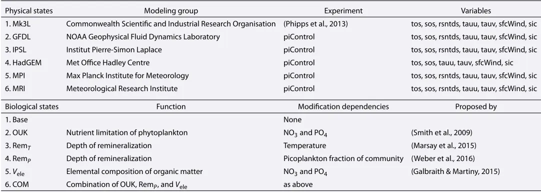
Figure 1.Taylor Diagram (Taylor, 2001) (correlation and normalized standard deviation) with additional color shading (normalized bias) displaying agreement between the simulated and observed fields of temperature (Temp), salinity (Sal), surface winds (Wind), mixed-layer depth (MLD), sea surface temperature (SST), and sea surface salinity (SSS) for all models. Models are represented by numbers: Mark 3L(1), Geophysical Fluid Dynamics Laboratory(2), Institut Pierre-Simon Laplace(3), Hadley Centre Global Environmental Model(4), Max Planck Institute for
Meteorology(5), and Meteorological Research Institute(6). Temperature and salinity observations come from the 1955–1964 reconstruction provided by the World Ocean Atlas (Locarnini et al., 2013; Zweng et al., 2013). Surface wind speed observations are the long-term from the National Centers for Environmental Prediction reanalysis of Kalnay et al. (1996). Mixed-layer depth observations are taken from the climatology of de Boyer Montégut et al. (2004). All fields are compared as annual averages.
4. Results
4.1. Physical States
All six physical states showed reasonable agreement in their global fields with observational data sets. Correlations ranged between 0.35 and 0.95 across all fields, and normalized standard deviations did not exceed 150% of the observations (Figure 1). Model-observation agreement was particularly good for the simu-lated sea surface temperature and whole-ocean temperature fields (0.93 < r2 < 0.95), with some states being over 1∘C warmer and others slightly cooler than the historical record (Table 2). Modest agreement was found for the sea surface and whole-ocean salinity fields (0.55 < r2 < 0.64). Again, some states were saltier and oth-ers fresher than the historical data. Surface wind speeds were also of modest agreement (0.53<r2<0.70), but all were too weak rela-tive to the National Centers for Environmental Prediction reanalysis data (Kalnay et al., 1996). The poorest model-data agreement was for mixed-layer depths (0.35<r2<0.43), which is a common result among skill assessments of climate models (Séférian et al., 2013). In this suite of experiments, the physical state driven by IPSL surface forcings was most correlated with the observations.
The six physical states formed deep water masses at rates simi-lar to observation-based estimates for the modern ocean (Table 2). The rate of AABW formation, which is a key driver of the lower over-turning cell and the properties of the deep ocean, varied from a minimum of 7.2 Sv in GFDL to a maximum of 15.1 Sv in IPSL and MRI. The multimodel mean rate of AABW formation was 12.3±3.0 Sv (mean±standard deviation), which is similar to the 12.5±4 Sv esti-mated by Lumpkin and Speer (2007) for 62∘S and an estimate of 14 Sv using chloroflurocarbons (Orsi et al., 2002). Therefore, all ocean states formed AABW within the range of observational error, with the exception of GFDL.
Table 2
Global Mean Temperature in∘C (Locarnini et al., 2013), Global Mean Salinity in Practical Salinity Unit (Zweng et al., 2013), and Estimates of Key Ocean Transports
in Sverdrups Taken From the Literature and Those Produced by the Models
Observations Mk3L GFDL IPSL HadGEM MPI MRI Model mean+SD Temp 3.7 4.0 5.4 5.0 3.6 3.6 4.7 4.4±0.7 Sal 34.7 34.5 34.7 34.9 34.4 34.4 34.4 34.6±0.2 AABWa 12.5±4 11.5 7.2 15.1 11.4 13.5 15.1 12.3±3.0 NADWb 18±5 18.4 20.3 14.8 13.0 16.7 13.9 16.2±2.8
NPIWc 2.3±0.1 11.1 11.7 12.7 11.8 12.1 17.2 12.8±2.2 Salinity min 953 m 1148 m 629 m 942 m 856 m 1067 m 1126 m 961±180 m SSIW subd 11.9 6.5 86.3 3.3 10.2 1.4 1.4 18.2±30.6
SSIW upwd 6.1 5.2 108.5 8.1 23.1 6.5 4.0 25.9±37.5
Note.The salinity minimum depth was calculated as the interpolated depth of the salinity minimum at 30∘S. See Appendix B for how the values were
calcu-lated. All values represent annual averages of the monthly metrics. Bold and italic numbers represent the strongest and weakest rates of circulation, respectively. SD = standard deviation; AABW = Antarctic Bottom Water; NADW = North Atlantic Deep Water; NPIW = North Pacific Intermediate Water; SSIW = Southern Source Intermediate Water; HadGEM = Hadley Centre Global Environmental Model; MPI = Max Planck Institute for Meteorology; MRI = Meteorological Research Institute; Mk3L = Mark 3L; IPSL = Institut Pierre-Simon Laplace; GFDL = Geophysical Fluid Dynamics Laboratory.
aEstimates from Lumpkin and Speer (2007) with the 14 Sv estimated by Orsi et al. (2002) falling within this range. bEstimates from Talley et al. (2003) with the
17±4.3 and 16±2 Sv of Lumpkin and Speer (2007) and Ganachaud (2003) falling within this range.cEstimates from Lumpkin and Speer (2007) and Talley et al.
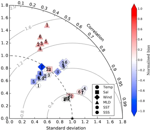
[image:8.612.36.576.540.659.2]Figure 2.The annual and zonal average of the global meridional overturning circulation for (a–f ) all six physical states. U:L represents the dominance of the upper overturning cell relative to the lower overturning cell, calculated by dividing the total area of positive velocities (Sv) by the total area of negative velocities (Sv) beneath 500 m. Note the stronger positive velocities in the upper overturning of MRI caused by greater formation rates of North Pacific Intermediate Water. HadGEM = Hadley Centre Global Environmental Model; MPI = Max Planck Institute for Meteorology; MRI = Meteorological Research Institute; GFDL = Geophysical Fluid Dynamics Laboratory; IPSL = Institut Pierre-Simon Laplace.
The production of NADW, which powers the upper overturning cell, also agreed with observational estimates. GFDL produced the strongest rate of NADW formation at 20.3 Sv, in contrast to its slow rate of AABW formation. The weakest rates of NADW formation were present in HadGEM and MRI at 13.0 and 13.9 Sv, respectively. The range of 13.0–20.3 Sv produced by the six ocean states agrees with the observational error of about 18±5 Sv (Talley et al., 2003), within which other estimates are accounted for (Ganachaud, 2003; Lumpkin & Speer, 2007).
The circulations of intermediate waters, however, showed some striking inconsistencies with observations. Simulated formation rates of NPIW were much greater than observations of∼2.3 Sv (Lumpkin & Speer, 2007; Talley et al., 2003). Hence, the ventilation of the North Pacific interior was too great for all states, especially MRI. Meanwhile in the Southern Hemisphere, the combined overturning of SSIW was highly variable in its rate and location. Rapid overturning in excess of 20 Sv at shallow depths were found in HadGEM and GFDL, par-ticularly GFDL, while less than 10 Sv of overturning associated with deeper salinity minima, more consistent with observations (Iudicone et al., 2011), were found in Mk3L, IPSL, MPI, and MRI states (Table 2). Of these, the Mk3L ocean state was the only state to produce net subduction of SSIW. The isopycnals associated with SSIW for these slower rates largely outcropped near the Antarctic coastline, despite deep convective mixing taking place in sub-Antarctic latitudes for all states. Thus, no single ocean state developed NPIW or SSIW dynamics consistent with observations, although some were less inconsistent than others.
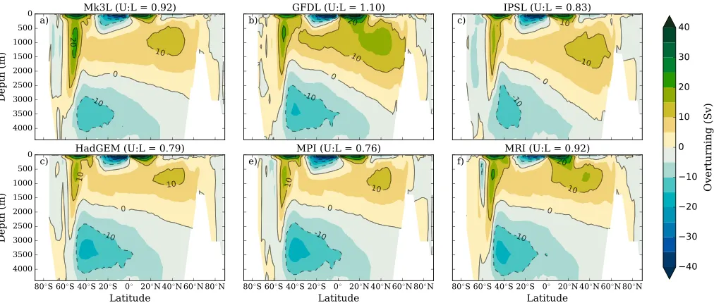
Figure 3.The relative influence of biological versus physical ocean states on major biogeochemical fields. Those fields with a slope<1 are those more sensitive to changes in physical conditions than biological function, and the steepness of the slope indicates the magnitude of sensitivity in either direction. The measure of influence is quantified as theFstatistic, which was produced by a ANOVA across the full contingent of physical and biological states in this study. Thus, there are six data points (Fstatistics) for each biogeochemical field in both the physical (xaxis) and biological (yaxis) space. The six data points alongxaxis, for instance, represent theFstatistic values that were generated by conducting ANOVA across all physical states for each biological state, while the six data points along theyaxis represent theFstatistic values that were generated across all biological states (Base, OUK, RemT, RemP,Vele, and COM) for each physical state. AllFstatistic values were highly significant (pvalue<0.005). DIC = dissolved inorganic carbon; ALK = alkalinity.
Our analysis of the ocean temperature and salinity fields shows a high level of agreement, while a lower level of agreement (albeit still relatively high) was found for other surface boundary conditions (Figure 1). The over-turning of important water masses showed a wide range of rates that were broadly consistent for deep waters and less so for intermediate waters. Global thermodynamic states and overturning were therefore plausibly representative of preindustrial conditions in the context of Holocene climate variability (Bond et al., 1997; Mayewski et al., 2004; Rasmussen et al., 2002), while subduction of intermediate waters was too weak in the Southern Ocean and too strong in the North Pacific.
4.2. Physical and Biological State Influence
One-way ANOVA of the major biogeochemical fields quantified how differences in physical and biological states affected their distributions.Fstatistics ranged between 25 and∼9,000 across the physical states and between 34 and 1,066 across the biological states (supporting information Table S2). The variance of each bio-geochemical field was significantly different between experiments (pvalues<0.005). To provide some context for the variation in biogeochemical fields, an ANOVA of purely physical fields showed a range of 320–2,582, with the least variability in temperature and the most in the salinity field. Because these fields were prescribed through a fixed surface climatology, this range represents the variation caused by physical differences. Addi-tionally, thephyO
2field produced anFstatistic of 816, which set a benchmark for changes caused solely by air-sea gas exchange and circulation. Ocean biogeochemistry was generally more sensitive to the physical state of the ocean than to changes in biological function. However, this sensitivity was dependent on the biogeochemical field in question.
O2and AOU clearly showed the greatest sensitivity, with at least tenfold the sensitivity to changes in the physical state than to changes in biological functioning (Figure 3). AOU was strongly influenced by phys-ical conditions because of its primary dependence on the circulation (residence time of water masses). Furthermore, O2and AOU showed a much greater range of variability under different physical states than the physical states themselves, includingphyO
2. This highlights how changes in the physical state also altered biological function, which had a multiplicative effect on oxygen values.
Figure 4.Taylor diagram (Taylor, 2001) displaying agreement between the simulated and observed nitrate field. The Taylor diagram depicts the correlation (angle), normalized standard deviation (radial distance from dashed line), and centered root-mean-square error (outward distance from reference star) between the simulated and observed fields. The small grey circles represent the Base biological state, and the grey line shows the change caused by the new biological state. Additional color shading to represent the normalized bias has been added. For reference, the standard deviation of the observed nitrate field was 9.4 mmol m−3. Observed nitrate data for which the simulated fields are compared to come from the World Ocean Atlas (Garcia, Locarnini, Boyer, Antonov,
Baranova et al., 2013). All fields are compared as annual averages.
PO4and NO3showed contrasting responses to physical and biological state changes, as PO4was more sen-sitive to physical change while NO3was more sensitive to biological change. PO4was roughly 2 to 4 times more sensitive to differences in physical conditions than in biological functioning. PO4showed very low sen-sitivity (Fstatistics≤333) to changes in biological function across the physical states. The distribution of NO3, however, was approximately 2 to 4 times more sensitive to changes in biological functioning than to changes in the physical state. NO3was the only biogeochemical field to be more strongly influenced by the biological state of the ocean than by physical conditions (Figure 3), and this apparent insensitivity occurred despite a wide spread of physical conditions (section 4.1).
4.3. Biological State Assessment
The biological state of the ocean had more influence over the distribution of NO3than changes in the physical state, making NO3unique. Changes to NO3therefore provided the clearest insight into which biological state was most representative of reality. Here we used the marine nitrogen cycle as the primary diagnostic with which to assess the performance of the different biological states.
4.3.1. Base
Table 3
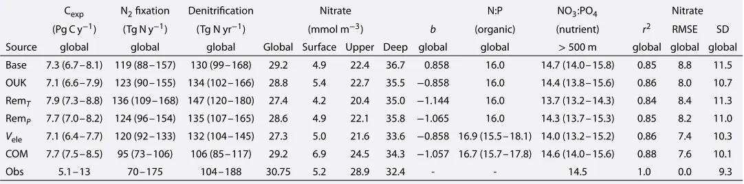
Key Diagnostics of the Oceanic Nitrogen Cycle and Biological Pump for All Biological States Described in Section 2.2 Relative to the Observations for the Modern Ocean
Cexp N2fixation Denitrification Nitrate N:P NO3:PO4 Nitrate (Pg C y−1) (Tg N y−1) (Tg N yr−1) (mmol m−3) b (organic) (nutrient) r2 RMSE SD Source global global global Global Surface Upper Deep global global >500 m global global global Base 7.3 (6.7–8.1) 119 (88–157) 130 (99–168) 29.2 4.9 22.4 36.7 0.858 16.0 14.7 (14.0–15.8) 0.85 8.8 11.5 OUK 7.1 (6.6–7.9) 123 (90–155) 134 (102–166) 28.8 5.4 22.7 35.5 −0.858 16.0 14.4 (13.8–15.6) 0.86 8.0 10.7 RemT 7.9 (7.3–8.8) 136 (109–168) 147 (120–180) 27.4 4.2 20.4 35.0 −1.144 16.0 13.7 (13.2–14.3) 0.84 8.4 11.3
RemP 7.7 (7.0–8.2) 124 (96–154) 135 (107–165) 28.6 4.9 22.1 35.8 −1.065 16.0 14.3 (13.7–15.3) 0.85 8.2 11.0
Vele 7.1 (6.4–7.7) 120 (92–133) 132 (104–145) 27.3 5.0 21.6 33.6 −0.858 16.9 (15.5–18.1) 14.0 (13.2–15.2) 0.86 7.4 10.3 COM 7.7 (7.5–8.5) 95 (73–106) 106 (85–117) 29.2 6.9 24.5 34.3 −1.057 16.7 (15.7–17.8) 14.6 (14.0–15.6) 0.88 7.6 10.1 Obs 5.1–13 70–175 104–188 30.75 5.2 28.9 32.4 - - 14.5 1.0 0.0 9.3
Note.Values are the mean across the six physical ocean states and the range in parentheses. Cexprefers to the annual export of particulate carbon from the surface
and includes general phytoplankton, calcifying plankton, and nitrogen fixers.brefers to the exponent used to set the steepness of the remineralization profile, otherwise known as a Martin curve (Martin et al., 1987). N:P is the stoichiometry of organic matter. NO3:PO4is the ratio of water column nitrate to phosphate. The global inventory of phosphate was 2.68 Pmol in all simulations. Observed nitrate concentrations and the NO3:PO4ratio of the interior ocean come from the World Ocean Atlas database (Garcia, Locarnini, Boyer, Antonov, Baranova et al., 2013). Observed rates of global denitrification are the range of estimates from Eugster and Gruber (2012). Observed rates of global carbon export production were generated by converting net primary production over the period 2003–2013 produced by the algorithms of Behrenfeld and Falkowski (1997) and Westberry et al. (2008) to carbon export from the euphotic zone using three independent conversions (Dunne et al., 2005; Henson et al., 2011; Laws et al., 2000). RMSE = root-mean-square error; SD = standard deviation.
for all physical states, with a multimodel mean of 0.85. Furthermore, the skill of the physical state was not a good predictor of its ability to simulate NO3, with the GFDL state producing the best NO3field.
However, a number of inconsistencies between the simulated and observed NO3fields were clearly present. Concentrations of NO3were underestimated in the upper ocean above 2,000 m by between 5 and 8 mmol m−3 on average (Figure 5). In the deep ocean below 2,000 m, NO3was overestimated by between 1 and 7 mmol m−3 on average, with the lower bound produced by GFDL, which had a very weak lower overturning cell. The error in the vertical distribution of NO3was found in all physical states, irrespective of circulation differences.
4.3.2. OUK
The implementation of optimal uptake kinetics (OUK) provided a consistent benefit to the NO3field by shifting NO3from the deep to the upper ocean (Figure 5). The key tenet of optimal uptake kinetics is that phyto-plankton adapt their internal physiology according to the availability of nutrients, reducing efficiency under nutrient-replete (eutrophic) conditions and increasing efficiency under nutrient-deplete (oligotrophic) con-ditions (Smith et al., 2009). Nutrient utilization in eutrophic regions decreased and delivered more NO3to oligotrophic regions, particularly from the subantarctic zone. This shifted nutrients from the deep to the upper ocean and partially rectified the systematic underestimation of upper ocean nutrients. The vertical shift was associated not only with roughly 0.6 mmol m−3increase in the average concentration of NO
3at the surface but also with a slight increase in the rate of denitrification that caused a global loss of∼0.4 mmol m−3. While the loss of NO3exacerbated the global negative bias, the change in distribution was beneficial across all physical states (Figure 4).
4.3.3. RemTand RemP
The introduction of spatial variations in organic matter remineralization also caused global shifts in NO3. However, the use of either temperature or phytoplankton-dependent parameterizations to control the remineralization profile (supporting information Figure S3) produced contrasting results.
The use of mesopelagic temperature to control remineralization (RemT) was detrimental. It increased the
transfer of organics to depth in the high latitudes while simultaneously increasing the recycling of organ-ics in the warm, low-latitude ocean. Approximately 12% more organic matter passed from the surface to 1,000 m depth in the Southern Ocean and Arctic, and this released large quantities of NO3into the deep ocean. Meanwhile, warmer temperatures in the lower latitudes produced shallower remineralization profiles, which increased export production (Cexp) by about 0.6 Pg C yr−1and the retention of NO3within the mesopelagic zone. Nutrients were therefore more efficiently recycled within the upper 500 m of the ocean, which increased global denitrification by∼18 Tg N yr−1and lead to a global loss of∼2 mmol NO
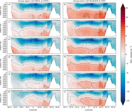
Figure 5.The zonal mean difference between the simulated and observed distributions of NO3(mmol m−3) for all biological state experiments. The
model-observation difference in NO3is shown for two contrasting ocean circulation types. The (a, c, e, g, i, k) strong upper cell is the combined average of GFDL and Mk3L NO3fields. The (b, d, f, h, j, l) strong lower cell is the combined average of HadGEM and MPI NO3fields. Figures 5a and 5b = Base experiments. Figures 5c and 5d = OUK experiments. Figures 5e and 5f = RemTexperiments. Figures 5g and 5h = RemPexperiments. Figures 5i and 5j =Veleexperiments.
Figures 5k and 5l = COM experiments.
lowered the interior NO3:PO4ratio from 14.7:1 to 13.7:1 well below observations of 14.5:1 (Garcia, Locarnini, Boyer, Antonov, Baranova et al., 2013). The combination of very deep remineralization profiles in the high latitudes with efficient nutrient recycling in the low latitudes largely exacerbated the initial biases (Figure 5).
In contrast, phytoplankton-dependent remineralization (RemP) slightly improved the simulated NO3field by shifting material from the deep to the upper ocean (Figure 5). The shift featured particularly in the Northern Hemisphere and occurred primarily because remineralization profiles shoaled relative to the Base exper-iments. The global averagebexponent varied between−1.06 and−1.08 among the RemPexperiments, retaining∼4% more organic matter within the upper 1,000 m compared to the−0.87 of the Base experiments (Martin et al., 1987). Because this increased the retention of nutrients at shallower depths, Cexpincreased by roughly 0.4 Pg C yr−1(Table 3). These changes caused a slight increase in denitrification rates. However, because the transfer of organics to depth in the equatorial zones was deep (b>−0.8), local export produc-tion decreased and dampened the global increase in denitrificaproduc-tion. Global NO3concentrations were reduced only slightly (0.5 mmol m−3), and the interior ocean NO
3:PO4ratio remained close to observations at 14.3:1.
4.3.4.Vele
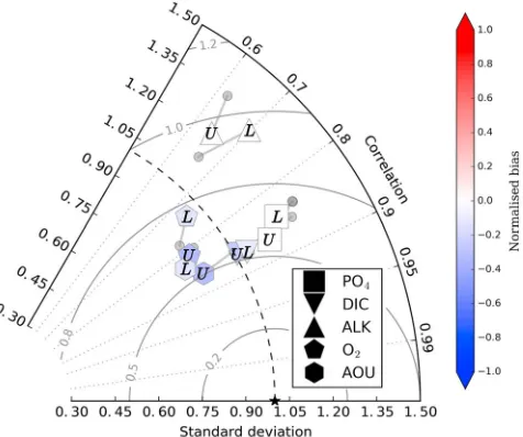
Figure 6.Taylor diagram (Taylor, 2001) displaying agreement between the simulated and observed fields of phosphate (PO4), dissolved inorganic carbon (DIC), alkalinity (ALK), dissolved oxygen (O2), and apparent oxygen utilization (AOU). Simulated fields include the mean of Mk3L and IPSL oceans, which have a strong upper overturning cell (U), and the mean of HadGEM and MPI, which have a strong lower overturning cell (L). GFDL and MRI ocean states were excluded because they formed important water masses outside of observational uncertainties (see section 4.1). The Taylor diagram depicts the correlation (angle), normalized standard deviation (radial distance from dashed line), and centered root-mean-square error (outward distance from reference star) between the simulated and observed fields. The small grey circles represent the Base biological state, and the grey line shows the change caused by the new biological state. Additional color shading to represent positive or negative changes in normalized bias due to the COM biological state has been added. For reference, the standard deviations of observations (mmol m−3) are PO
4= 0.68, DIC = 91.4,
ALK = 43.0, O2= 64.7, and AOU = 67.4. Nutrient and oxygen observations come from the World Ocean Atlas (Garcia, Locarnini, Boyer, Antonov, Mishonov et al., 2013; Garcia, Locarnini, Boyer, Antonov, Baranova et al., 2013), and carbon data come from the Global Ocean Data Analysis Project (Key et al., 2004). All fields are compared as annual averages.
raised relative to the Redfield ratio of 16:1 for most of theVeleexperiments, giving a multimodel average of 16.9:1 (Table 3). Regionally, N:P ratios were lowest in the Southern Ocean (8:1) and in other eutrophic regions, while oligotrophic waters, particularly the North Atlantic and Northern Indian Oceans, were highest (25:1). Likewise, Nden:P ratios were lowered from 94.4 to 70–80 mmol m−3in eutrophic regions, such as the Eastern Equatorial Pacific, but increased within suboxic zones that were overlain with nutrient-deplete waters (supporting information Figure S4).
These large-scale variations in N:P and Nden:P improved the NO3 distribu-tion for all physical states (Figure 4) and did so for two reasons. First, the NO3inventory of the lower overturning cell was strongly reduced, which rectified the overestimation of NO3in the deep ocean. The loss of NO3 from the lower overturning cell was caused by low N:P ratios in the South-ern Ocean. Low NO3uptake by Southern Ocean phytoplankton reduced the local export of nitrogen to depth, which allowed more NO3to exit the lower overturning cell via southern source intermediate waters. The result was a continued loss of the NO3from the lower overturning cell to the upper overturning cell.
Second, the loss from the deep ocean was not accompanied by a loss from the upper ocean, which remained relatively unchanged in NO3content. The conservation of NO3was related to lower Nden:P ratios that reduced denitrification rates. In the Eastern Equatorial Pacific, more NO3upwelled to the surface due to low denitrification rates. This enforced a positive feedback mechanism, whereby low N:P ratios at the surface decreased Nden:P ratios, and in turn increased NO3delivery to the surface, which fur-ther lowered N:P ratios. These changes accumulated NO3within the upper Pacific Ocean.
However, low Southern Ocean N:P ratios caused significant losses in the oceanic NO3reservoir of 25 to 50 Pg N (1.4–2.8 mmol m−3), leading to a consistent negative bias. This loss occurred because more NO3 was allowed to exit the lower cell and subsequently cycled through deni-trification zones. Interestingly, lower NO3 reservoirs developed despite mean N:P ratios that largely exceeded the Redfield ratio (Table 3), which demonstrated the importance of the lower cell for nutrient storage. The consequence was a detrimental change in the NO3:PO4ratio of the interior ocean from approximately 14.7:1 in theBaseexperiments to∼13.9:1.
4.3.5. COM
The COM biological state provided the best simulated-observed agreement in the NO3field. Correlations were the highest with a mean of 0.88, standard deviations were brought much closer to observations, and the root-mean-square error was minimized to less than 0.6 standard deviations (Table 3).
The combination of OUK, RemP, andVeleproduced contrasting responses between eutrophic and oligotrophic environments that allowed NO3to shift from the deep to the upper ocean without incurring a loss in the NO3 inventory (Figure 5). In eutrophic regions, OUK andVeleweakened export production, RemPsubsequently
4.4. Other Biogeochemical Fields
The COM biological state provided the greatest benefit to NO3, and we tested its effect on other major biogeo-chemical fields. For this we placed more importance on the PO4, DIC, and ALK fields, as these fields showed a lesser sensitivity to physical changes than O2and AOU (Figure 3). Improvements in PO4were particularly telling of improvements in the biogeochemical model because this field had no external sources or sinks to or from the ocean.
COM improved the simulated fields of PO4, DIC, and ALK in those oceans with a stronger upper cell, while also providing slight improvements to PO4and DIC for oceans with a strong lower cell (Figure 6). These fields were improved in their correlation, normalized standard deviation, and/or root-mean-square error relative to the observations provided by WOA and Global Ocean Data Analysis Project data sets (Garcia, Locarnini, Boyer, Antonov, Baranova et al., 2013; Garcia, Locarnini, Boyer, Antonov, Mishonov et al., 2013; Key et al., 2004). The distributions of PO4, DIC, and ALK showed the greatest improvement in strong upper cell oceans, while improvements to ALK and oxygen species (O2and AOU) were small or even negative for the oceans with a stronger lower cell (HadGEM and MPI). Importantly, the PO4and DIC fields showed consistent improvement for both circulation types.
The improvements in PO4and DIC mirrored those of NO3, as material shifted from the deep to the upper ocean (supporting information Figure S5). This reduced the bias between the simulated and observed values, particularly for oceans with the stronger upper cell, which were oceans that better fit the observed physical fields (see section 4.1). PO4and DIC were relocated from the deep ocean into the upper ocean as greater quantities of these species left the lower overturning circulation via the same mechanisms as NO3. For DIC, the shift of material into the upper ocean increased the loss of carbon via air-sea gas exchange, and between 125 and 400 Pg C was lost depending on the physical state. This loss rectified the initial overestimation in the deep ocean but did little to resolve an underestimation of DIC in the upper ocean. Overall, however, the COM biological state gave a consistent improvement in the PO4and DIC fields across a range of physical states.
4.5. Response of the Carbon and Nitrogen Cycles
Consistent improvement in the simulated-observed agreement for NO3, PO4, DIC, and ALK provided evidence that COM best represented the functioning of the marine biological community. We therefore evaluated the sensitivity of improved carbon and nitrogen cycles to variation in the ocean’s physical state.
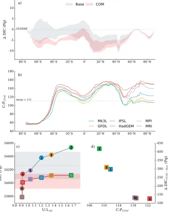
The COM biological state reduced differences in global carbon export between the physical states by roughly 0.4 Pg C yr−1(Table 3) and reduced differences in global carbon content between physical states by∼50% (Figure 7). These changes occurred via an interaction between nutrient delivery to the surface and the stoi-chiometry of organic matter. Those oceans with a weaker AMOC (U:LAtl≤1.0), which included HadGEM, MPI, and MRI ocean states, had weaker global rates of export production under the Base biological state. Under the COM biological state, however, more nutrients were delivered to surface waters, which increased biological consumption of PO4, increased local C:P ratios throughVele, and further enhanced carbon export. The degree of nutrient limitation in a given physical state was proportional to the increase in global C:P ratios (Figure 7), and this relationship minimized the multimodel spread in biological carbon sequestration. Losses of DIC from all physical states due to the shift of material into the upper ocean, coupled with lower C:P ratios over deep water formation regions, also contributed to greater similarity. Losses occurred in every major oceanic basin, but those oceans with higher C:P ratios (stratified oceans) limited carbon outgassing. As a result of these changes, the range in oceanic carbon inventories halved from 616 Pg C in the Base biological state to 327 Pg C in the COM biological state. In fact, all physical states held roughly 34,000–34,100 Pg C, with the exception of the∼33,800 Pg C contained within MRI, which reflected reduced storage capacity in the North Pacific due to strong seasonal ventilation by NPIW (see section 4.1).
Figure 7.Changes in the total carbon content of the ocean and its major driver between the Base (grey shading) and combination (COM, pink shading) biological states. (a) The difference between the simulated and observed (Key et al., 2004) zonally integrated carbon content (Pg C) is shown for both biological states, with the shading representing one standard deviation either side of the mean across all physical states. (b) The zonally averaged C:P ratios of the COM biological state. (c) How the total carbon content of each ocean state changed between the Base (circles; grey shading) and COM (squares; pink shading). Each ocean state lost carbon under the COM biological state as material was shifted into the upper ocean and carbon was subsequently lost to the atmosphere. (d) How the magnitude of loss was mitigated by the magnitude of increase in the global mean C:P ratio, such that differences in carbon content were minimized across physical states. Physical states are Mk3L(1), GFDL(2), IPSL(3), HadGEM(4), MPI(5), and MRI(6).
Under the COM biological state, however, this relationship was eroded (Figure 8), and inter-ocean differences in NO3content decreased from 74 Pg N to 57 Pg N.
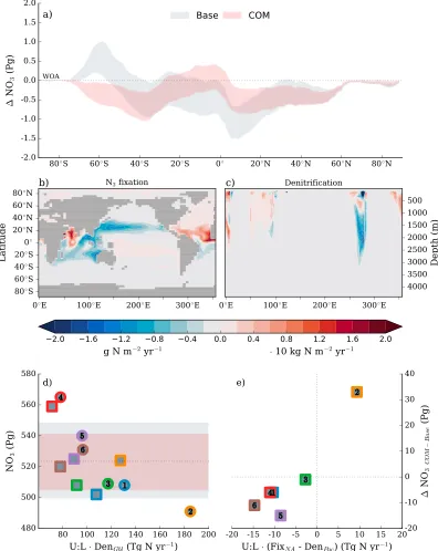
Figure 8.Changes in the total nitrogen content of the ocean and its major driver between the Base (grey shading) and combination (COM, pink shading) biological states. (a) The difference between the simulated and observed (Garcia, Locarnini, Boyer, Antonov, Baranova et al., 2013) zonally integrated nitrate content (Pg N) is shown for both biological states, with the shading representing one standard deviation either side of the mean across all physical states. (b) The depth integrated difference in nitrogen fixation (g N m−2yr−1) between the COM and Base biological states. (c) The meridional integrated difference in denitrification (⋅10 kg N m−2yr−1) between the COM and Base biological
The fact that GFDL was dominated by a strong upper overturning cell augmented the accumulation of NO3in the upper Pacific under these conditions and more than offset the losses from the deep ocean caused by low Southern Ocean nitrogen export. In other oceans, a decrease in Pacific denitrification and an increase in North Atlantic nitrogen fixation was insufficient to offset the losses from the lower overturning cell. Importantly though, these regional responses in nitrogen fixation and denitrification to the physical conditions ensured that losses in global NO3storage were minimized.
5. Discussion
We have made three major findings in this model study. First, the marine nitrogen cycle is highly sensi-tive to marine biological processes and therefore provides a powerful tool for assessing the performance of biogeochemical ocean models. Second, the simulation of ocean biogeochemistry is significantly improved by allowing the marine community to respond dynamically to its environment. Third, including dynamical biological functioning reduces the sensitivity of the carbon and nitrogen cycles to changes in the ocean’s physical state.
The biogeochemical parameterizations that were tested (see section 2) are simplistic when compared to the rich diversity of planktonic marine life and their complex interactions (see Worden et al., 2015, for a review). However, they expressed important features of ocean biology in an implicit way. Unproductive regions, such as the subtropical gyres, are dominated by picoplankton (Hirata et al., 2011; Kostadinov et al., 2009). These oligotrophic communities are represented in the majority byProchlorococcusandSynechococcusand are associated with (1) high growth rates despite strongly nutrient limited conditions in the environment (Liu et al., 1997), (2) high rates of regenerated production supporting low rates of export production to the deep ocean (Henson et al., 2012; Mouw et al., 2016; Worden et al., 2004), and (3) higher stoichiometric requirements of nitrogen and carbon per unit of phosphorus (Klausmeier et al., 2004). In contrast, more pro-ductive regions are known to be dominated by large phytoplankton types, such as diatoms (Hirata et al., 2011; Kostadinov et al., 2009), and are associated with (1) relatively slower nutrient uptake rates given the nutrient-replete conditions (Gotham & Rhee, 1981a, 1981b; Smith & Yamanaka, 2007), (2) a more efficient transfer of less labile material to depth (Henson et al., 2012; Mouw et al., 2016), and (3) lower stoichiometric requirements of carbon and nitrogen per unit phosphorus (Klausmeier et al., 2004; Weber & Deutsch, 2010). In addition to these general patterns, a wide range of observed transfer efficiencies in the high latitudes (Boyd & Trull, 2007; Buesseler et al., 2007) and the efficient transfer of organics from areas overlying oxygen-poor zones (Cavan et al., 2017) were resolved. The combination of OUK (Smith et al., 2009), RemP(Weber et al., 2016), andVele(Galbraith & Martiny, 2015) therefore reproduced regional features of the global marine community and did so via either a direct or indirect relationship to nutrient concentrations. These patterns are consistent with an emerging understanding that variations in the biological community are important for controlling major biogeochemical cycles in the ocean (Le Quéré et al., 2005; Worden et al., 2015).
With that being said, our simulations excluded some key processes that may have contributed to the original bias in the Base biogeochemical fields. The major biogeochemical process that was excluded was sedimen-tary denitrification. Sedimensedimen-tary denitrification is the largest contributor to the global rate of fixed nitrogen loss and is estimated to be roughly 1.8-fold that of pelagic denitrification (Eugster & Gruber, 2012). Applying this ratio to the denitrification rates of the Base biological state gives sedimentary and pelagic denitrifica-tion rates of 64–108 Tg N yr−1and 35–60 Tg N yr−1, respectively, which bare striking resemblance to the observation-constrained estimates of Eugster and Gruber (2012). Spreading NO3losses across a greater spa-tial extent via sedimentary denitrification may therefore have reconciled the overestimation of NO3in the deep ocean. However, the bulk of sedimentary NO3loss is known to occur primarily in water depths less than 1,000 m (Gruber & Sarmiento, 1997). Due to the coarse resolution of our OGCM and its overestimation of anoxic water, much pelagic denitrification already occurred at depths where sedimentary denitrification is known to occur. While we cannot unequivocally say that the inclusion of sedimentary denitrification would not be beneficial, we argue that its inclusion would only marginally rectify the deep upper ocean NO3bias.
Important physical processes were also not accounted for in the simulations due to the coarse resolution of the ocean model. Mesoscale and submesoscale motions, such as eddy-induced stirring and turbulence, are important to reproduce a credible large-scale circulation. The 2.8∘in longitude by 1.6∘in latitude grid spac-ing of the OGCM is larger than any resolution required to adequately resolve these dynamics (Hallberg, 2013). The inconsistencies between simulated and observed overturnings of intermediate waters in the North Pacific and Southern Ocean are testament to this fact. All ocean states, except the Mk3L, produced net upwelling of intermediate waters in the Southern Ocean in contrast with estimates (Iudicone et al., 2011). Intermediate waters are a major supply of nutrients to the mesopelagic ocean (Sarmiento et al., 2004), and the inability of each physical state to generate realistic subduction rates likely contributed to the vertical bias in nutrients that was common across all states. The overturning circulations were also biased by an unrealistic forma-tion of Southern Ocean dense waters via convective mixing in the open ocean, rather than on the Antarctic shelves (Heuzé et al., 2013). The multiple circulations shared the same model physics and architecture, and it is therefore unsurprising that all circulations featured the same biases, albeit to a greater or lesser extent.
Nonetheless, the inclusion of dynamic biological functioning improved the distribution of NO3markedly. It also altered the response of the NO3reservoir to physical change, dampening its sensitivity. Under the Base biological state, the oceanic inventory of NO3could be predicted by taking the product of the circulation type, U:L (see section 4.1), and the global denitrification rate, DenGbl(see section 4.5). However, this simple rela-tionship was eroded under the COM biological state as the NO3inventory became more dependent on how biology responded to its environment. The NO3content of the deep ocean was set by the N:P ratio over the Southern Ocean. Variable stoichiometry (Vele) allowed those oceans dominated by a more voluminous and nutrient-rich lower cell to develop lower N:P ratios, and these states lost more NO3. In contrast, the NO3 con-tent of the upper ocean was set by basin-specific rates of nitrogen fixation and denitrification. Stratified oceans with weaker nutrient delivery (U:LAtl ≤1) experienced stronger increases in nitrogen fixation, particularly in the North Atlantic, as higher N:P ratios increased the competitive advantage of nitrogen fixers (Landolfi et al., 2015). Meanwhile, oceans with stronger nutrient delivery experienced reduced denitrification, particularly in the Pacific, as Nden:P values were lowered. These biological responses to physical conditions increased North Atlantic sources from 14–66 to 29–64 Tg N yr−1and decreased Pacific sinks from 67–32 to 25–20 Tg N yr−1 between the Base and COM experiments. The role of the North Atlantic as afactory of fixed nitrogen, which exports the majority of its newly fixed nitrogen into NADW (McGillicuddy, 2014), and the role of the Pacific as aleaking storage warehousewere therefore made more similar across different physical states. We have some confidence that these changes are reasonable reflections of reality because they were associated with a sig-nificant improvement in the simulated NO3field, although rates of nitrogen fixation for the Pacific were too low compared to observations (Luo et al., 2012). However, the relative rate of sources and sinks and their loca-tions within each basin are important for the NO3inventory. In addition to the necessity of non-Redfield ratios (Weber & Deutsch, 2012), we therefore also support the conclusions of Weber and Deutsch (2014) in that basin-specific rates of nitrogen fixation and denitrification are important for setting the oceanic inventory of fixed nitrogen. But we extend and combine these theories in the context of dynamic biological functioning under different circulation states, where dynamic biological functioning under different physical conditions helps to stabilize the NO3content of the ocean.