Market segmentation analysis

(1)

This is a repository copy of Market segmentation analysis. White Rose Research Online URL for this paper:

http://eprints.whiterose.ac.uk/2061/

Monograph:

Whelan, G. and Bates, J. (2001) Market segmentation analysis. Working Paper. Institute of Transport Studies, University of Leeds , Leeds, UK.

Working Paper 565

[email protected] https://eprints.whiterose.ac.uk/ Reuse

See Attached

Takedown

If you consider content in White Rose Research Online to be in breach of UK law, please notify us by

(2)

White Rose Research Online

http://eprints.whiterose.ac.uk/

Institute of Transport Studies

University of Leeds

This is an ITS Working Paper produced and published by the University of Leeds. ITS Working Papers are intended to provide information and encourage discussion on a topic in advance of formal publication. They represent only the views of the authors, and do not necessarily reflect the views or approval of the sponsors.

White Rose Research Online_{URL for this paper:}

http://eprints.whiterose.ac.uk/2061/

Published paper

G Whelan, J Bates (2001) Market Segmentation Analysis. Institute of Transport Studies, University of Leeds, Working Paper 565

(3)

CONTENTS

1. Introduction... 2

2. Base Models... 2

3. Income Effects ... 3

4. Journey Distance... 6

5. Reimbursement ... 9

6. Fraction of travel time in congested conditions ... 10

7. Vehicle occupancy ... 11

8. Trip sub-purposes... 11

9. Occupation ... 12

10. Age group... 13

11. Gender... 13

12. Household Type ... 14

13. Free time ... 14

14. Passenger or Driver... 15

15. Fixed Arrival Time ... 16

16. Area Type... 16

17. Full Segmentation Models ... 17

18. Direct Estimation of Elasticities ... 21

19. Elasticity Segmentation by Household Size ... 22

20. Conclusions... 24

(4)

1. INTRODUCTION

This working paper presents the findings of research aimed at assessing differences in the value of time by market segment. It draws on findings presented in AHCG’s final report to DETR (AHCG, 1996) and previous research conducted during the course of this research contract (Bates and Whelan, 2001) and it is intended that this document be read in conjunction with those two reports.

The paper describes the estimation of a base model for each journey-purpose (business, commuting and other) and shows how each is influenced by: income, journey distance, cost reimbursement, congestion, vehicle occupancy, trip sub-purpose, occupation, age group, gender, household type, ‘free time’, respondent type, time constraints and geographical region. The findings of this analysis are then drawn together to develop a final set of models that allow the value of time to vary across a range of market segments. All models are estimated using GAUSS (Aptech Systems) without taking account of the repeat observations nature of the stated preference data.

2. BASE MODELS

Following Bates and Whelan (2001), the base models have three key features: • an inertia term that takes account of the sign effects;

• a ‘perception filter’ that addresses the size effect; and • journey cost co-variates to account for ‘budget effects’

The proposed basic form of the utility function is therefore:

Uikj = βc0. Δcikj + βcC.Ci .Δcikj + βt0. Δτikj + Ω Itckj

Where Δτ is the ‘perceived’ time difference with the formula: Δτ = Sign (Δt) * { |Δt| . [ |Δt| ≥ θ] + θ.( |Δt|/θ)M_{. [ |Δt| < θ] }}

where τ is perceived time, θ is a ‘threshold’ value, and m > 1 an estimated parameter.

Here and henceforth, a term of the form [condition] represents a logical (dummy) variable with the value 1 if the condition is satisfied, 0 otherwise.

Table 1 shows the coefficient estimates and associated statistics for the base model for each journey-purpose. Before discussing the results, it is worth noting that the threshold parameter (θ) was constrained to equal 11 minutes in each model; this value generates the best level of fit when compared with model runs with other integer values for θ.

(5)

[image:5.612.84.513.91.246.2]

Table 1: Base Models

Business Commute Other

Δτ -0.09062441 (28.21) -0.10564560 (14.09) -0.08638727 (20.52) M 3.14995188 (7.19) 4.43513312 (4.42) 8.20231608 (7.45)

Theta 11.0 (fixed) 11.0 (fixed) 11.0 (fixed)

Δc -0.00984254 (22.06) -0.01667671 (18.77) -0.01709972 (27.71) Inertia 0.82229033 (24.84) 0.89138218 (18.20) 0.96458147 (25.09) Δc.C /10000 0.01709845 (6.76) 0.02611647 (3.29) 0.03448394 (9.98)

Observations 9557 4737 8038

Final likelihood -5776.47 -2758.70 -4528.15

Mean likelihood -0.604423 -0.582373 -0.563342

Please note the mean likelihood is the likelihood per observation.

For each journey-purpose the coefficient estimates have plausible relative magnitudes and all are estimated with a high degree of precision. For time changes greater than or equal to the threshold value M the value of time is given by:

VOT = βt0 / (βc0 + βcC.C )

Using average journey costs of 822.9, 301.5 and 623.4 pence for business, commute and other traffic, the values of time are 10.74, 6.65 and 5.78 pence per minute respectively. Other things equal, respondents favour the ‘as now’ position (as shown by the inertia term) by 97.48, 56.10 and 64.52 pence for business, commuting and other traffic respectively. With regard to small time savings, the M parameters demonstrate that business respondents have the highest perception of small time changes and ‘other’ traffic the lowest perception. Finally, the cost covariate shows a relatively strong relationship between journey distance [proxied by journey cost] and the value of time, with long distance travellers revealing higher values of time. All in all, the base models provide a solid foundation from which to assess other factors that may influence the value of time.

3. INCOME EFFECTS

Analysis of how household income (Y) affects the value of time has been achieved using both category (income is defined within 7 groups) and absolute effects. In other words, the specification is either:

Uikj = [βc0 + Σr>1 βcr [Y=r] ]. Δcikj + [βcC0 + Σr>1 βcCr [Y=r]].Ci .Δcikj + ...

or Uikj = [βc0 + βcY Yi ]. Δcikj + [βcC0 + βcCY Yi] .Ci .Δcikj + ...

The first set of models shown in Table 2 look at the impact of income on choice, whereas the second set of models, shown in Table 3, take additional consideration of the interaction between income and journey cost on choice; this accounts for the fact that

(6)

[image:6.612.82.514.115.366.2]

high income households generally travel further than low income households. Both models define Income group 1 as the base.

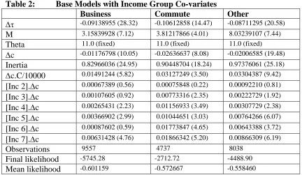
Table 2: Base Models with Income Group Co-variates

Δτ -0.09138955 (28.32) -0.10612858 (14.47) -0.08711295 (20.58) M 3.15839928 (7.12) 3.81217866 (4.01) 8.03239107 (7.44) Theta 11.0 (fixed) 11.0 (fixed) 11.0 (fixed) Δc -0.01176798 (10.05) -0.02636637 (8.08) -0.02006585 (19.48) Inertia 0.82966036 (24.95) 0.90448704 (18.24) 0.97376061 (25.18) Δc.C/10000 0.01491244 (5.82) 0.03127249 (3.50) 0.03304387 (9.42) [Inc 2].Δc 0.00067389 (0.56) 0.00075848 (0.22) 0.00092210 (0.81) [Inc 3].Δc 0.00107605 (0.92) 0.00773316 (2.35) 0.00222729 (1.92) [Inc 4].Δc 0.00265431 (2.23) 0.01156933 (3.49) 0.00307729 (2.38) [Inc 5].Δc 0.00366902 (2.99) 0.01044651 (3.03) 0.00764266 (6.07) [Inc 6].Δc 0.00087602 (0.59) 0.01773847 (4.65) 0.00643388 (3.72) [Inc 7].Δc 0.00631428 (4.76) 0.01866342 (5.20) 0.00866309 (6.19)

Mean likelihood -0.601159 -0.572667 -0.558460 Looking at the coefficients for income group1 in Table 2, it is clear that respondents from higher income households have higher values of time, since their effect is to reduce the disutility of cost. This trend is generally monotonic and could be approximated by a simple linear trend in the utility function (βYΔc) in which household income is specified as the mid-point of the relevant income group. The effect of income on the value of time is strongest for commuters and weakest for business traffic.

The models shown in Table 3 build on those presented in Table 2 by adding an interaction term between income group and overall journey cost. Although we might expect higher income respondents to travel further than lower income households it is hard to see strong patterns in the coefficient values. In principle we would expect all the income related coefficients to be positive, though this is not always the case. Perhaps we are asking too much from the data.

1

Income Group 1 = £10,000 or less p.a. with an assumed mean value of £5,000 Income Group 2 = £10,001 – £20,000 p.a. with an assumed mean value of £15,000 Income Group 3 = £20,001 – £30,000 p.a. with an assumed mean value of £25,000 Income Group 4 = £30,001 – £40,000 p.a. with an assumed mean value of £35,000 Income Group 5 = £40,001 – £50,000 p.a. with an assumed mean value of £45,000 Income Group 6 = £50,001 – £60,000 p.a. with an assumed mean value of £55,000 Income Group 7 = greater that £60,000 p.a. with an assumed mean value of £75,000

(7)

[image:7.612.86.517.94.431.2]

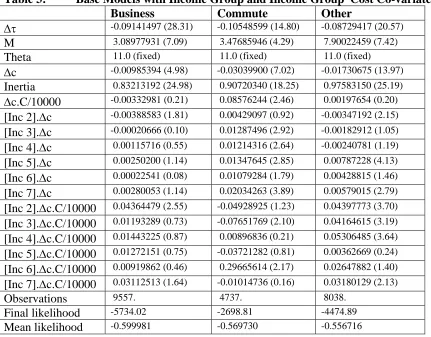
Table 3: Base Models with Income Group and Income Group*Cost Co-variates Business Commute Other

Δτ -0.09141497 (28.31) -0.10548599 (14.80) -0.08729417 (20.57) M 3.08977931 (7.09) 3.47685946 (4.29) 7.90022459 (7.42) Theta 11.0 (fixed) 11.0 (fixed) 11.0 (fixed) Δc -0.00985394 (4.98) -0.03039900 (7.02) -0.01730675 (13.97) Inertia 0.83213192 (24.98) 0.90720340 (18.25) 0.97583150 (25.19) Δc.C/10000 -0.00332981 (0.21) 0.08576244 (2.46) 0.00197654 (0.20) [Inc 2].Δc -0.00388583 (1.81) 0.00429097 (0.92) -0.00347192 (2.15) [Inc 3].Δc -0.00020666 (0.10) 0.01287496 (2.92) -0.00182912 (1.05) [Inc 4].Δc 0.00115716 (0.55) 0.01214316 (2.64) -0.00240781 (1.19) [Inc 5].Δc 0.00250200 (1.14) 0.01347645 (2.85) 0.00787228 (4.13) [Inc 6].Δc 0.00022541 (0.08) 0.01079284 (1.79) 0.00428815 (1.46) [Inc 7].Δc 0.00280053 (1.14) 0.02034263 (3.89) 0.00579015 (2.79) [Inc 2].Δc.C/10000 0.04364479 (2.55) -0.04928925 (1.23) 0.04397773 (3.70) [Inc 3].Δc.C/10000 0.01193289 (0.73) -0.07651769 (2.10) 0.04164615 (3.19) [Inc 4].Δc.C/10000 0.01443225 (0.87) 0.00896836 (0.21) 0.05306485 (3.64) [Inc 5].Δc.C/10000 0.01272151 (0.75) -0.03721282 (0.81) 0.00362669 (0.24) [Inc 6].Δc.C/10000 0.00919862 (0.46) 0.29665614 (2.17) 0.02647882 (1.40) [Inc 7].Δc.C/10000 0.03112513 (1.64) -0.01014736 (0.16) 0.03180129 (2.13)

Observations 9557. 4737. 8038.

Mean likelihood -0.599981 -0.569730 -0.556716

The models shown in Table 3 can be simplified by specifying two income covariates: βYΔc and βYCΔc. The first picks up the effect of income on the value of time and the second looks at the interaction between income and journey distance. From the results presented in Table 4, it can be seen that income has a significant positive effect on the value of time but the income-journey costs interaction is insignificant, though only marginally so for commuters. The income values used are those given in footnote 1, divided by 1000.

The relationship between income and the value of time is returned to in section 18 of this working paper where we estimate income elasticities.

(8)

[image:8.612.84.514.75.263.2]

Table 4: Base Models with Income and Income*Cost Co-variates

Δτ -0.09121656 (28.30) -0.10654543 (14.43) -0.08717604 (20.61) M 3.14767989 (7.13) 3.89331958 (4.00) 8.03403697 (7.46) Theta 11.0 (fixed) 11.0 (fixed) 11.0 (fixed) Δc -0.01346253 (15.01) -0.02583073 (13.81) -0.02107306 (21.03) Inertia 0.82593445 (24.87) 0.90467384 (18.26) 0.97335445 (25.19) Δc C/10000 0.02174806 (3.55) -0.00688166 (0.31) 0.03010628 (4.98) Income.Δc 0.00012001 (4.85) 0.00025105 (5.03) 0.00014679 (5.14) Income.Δc.C/10000 -0.00021713 (1.28) 0.00140301 (1.87) 0.00009572 (0.51)

Observations 9557 4737. 8038.

Mean likelihood -0.601939 -0.573393 -0.558881

4. JOURNEY DISTANCE

[image:8.612.82.512.419.713.2]

Bates and Whelan (2001) indicate that the value of time is related to journey length. Because information on journey distance was not collected during the survey we have to proxy distance by journey time or cost. On the basis of the evidence provided in tables 5 to 8 we recommend that journey cost is used as the distance covariate on cost changes. In Tables 5 and 6 the base cost and time coefficients (respectively) relate to a journey cost under £1, while in Tables 7 and 8 the base cost and time coefficients (respectively) relate to a journey time under 20 minutes.

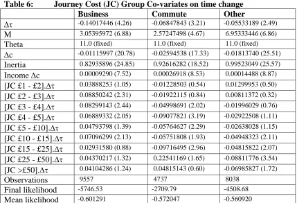
Table 5: Journey Cost (JC) Group Co-variates on cost change

Δτ -0.08999346 (28.13) -0.10671864 (15.81) -0.08334794 (19.75) M 2.42574248 (7.06) 2.15689470 (6.39) 7.09274013 (6.76) Theta 11.0 (fixed) 11.0 (fixed) 11.0 (fixed) Δc -0.01879905 (6.15) -0.04296527 (10.36) -0.03412553 (10.83) Inertia 0.83119734 (24.92) 0.90811254 (18.13) 0.97630810 (25.06) Income.Δc 0.00008840 (7.14) 0.00024218 (7.61) 0.00012350 (7.65) [JC £1 - £2].Δc 0.00600102 (1.73) 0.00971239 (2.42) 0.00635065 (1.83) [JC £2 - £3].Δc 0.00154168 (0.40) 0.01495929 (3.77) 0.01303463 (3.94) [JC £3 - £4].Δc 0.00159063 (0.50) 0.01819180 (4.48) 0.01396927 (4.12) [JC £4 - £5].Δc 0.00460585 (1.47) 0.02334276 (5.58) 0.01571557 (4.57) [JC £5 - £10].Δc 0.00592070 (1.86) 0.02310669 (5.72) 0.01704132 (5.39) [JC £10 - £15].Δc 0.00588401 (1.92) 0.02139542 (4.89) 0.02043955 (6.42) [JC £15 - £25].Δc 0.00954617 (3.10) 0.02729146 (6.18) 0.01923659 (6.03) [JC £25 - £50].Δc 0.00848715 (2.79) -0.14503678 (1.43) 0.02336491 (7.20) [JC >£50].Δc 0.00897099 (2.96) -0.00280611 (0.12) 0.02281241 (5.26)

Mean likelihood -0.599398 -0.563973 -0.554287

(9)

[image:9.612.84.513.101.394.2]

Table 6: Journey Cost (JC) Group Co-variates on time change

[image:9.612.86.511.418.707.2]

Δτ -0.14017446 (4.26) -0.06847843 (3.21) -0.05533189 (2.49) M 3.05395972 (6.88) 2.57247498 (4.67) 6.95333446 (6.86) Theta 11.0 (fixed) 11.0 (fixed) 11.0 (fixed) Δc -0.01115997 (20.78) -0.02594538 (17.33) -0.01813740 (25.51) Inertia 0.82935896 (24.85) 0.92616282 (18.52) 0.99523049 (25.57) Income Δc 0.00009290 (7.52) 0.00026918 (8.53) 0.00014488 (8.87) [JC £1 - £2].Δτ 0.03888253 (1.05) -0.01228503 (0.54) 0.01299953 (0.50) [JC £2 - £3].Δτ 0.08850242 (2.31) -0.01922115 (0.84) 0.00811372 (0.32) [JC £3 - £4].Δτ 0.08299143 (2.44) -0.04998691 (2.02) -0.01996029 (0.76) [JC £4 - £5].Δτ 0.06889332 (2.05) -0.09077821 (3.19) -0.02922508 (1.11) [JC £5 - £10].Δτ 0.04793798 (1.39) -0.05764627 (2.29) -0.02638028 (1.15) [JC £10 - £15].Δτ 0.07096299 (2.13) -0.05751808 (1.93) -0.04948323 (2.11) [JC £15 - £25].Δτ 0.02931580 (0.88) -0.09716495 (2.96) -0.04815822 (2.07) [JC £25 - £50].Δτ 0.04370217 (1.32) 0.22541169 (1.65) -0.08811776 (3.54) [JC >£50].Δτ 0.04104286 (1.24) 0.04815143 (0.60) -0.06985827 (1.72)

Mean likelihood -0.601291 -0.572047 -0.560920

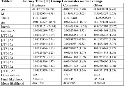
Table 7: Journey Time (JT) Group Co-variates on cost change

Δτ -0.09008631 (28.14) -0.02084306 (3.00) -0.08278312 (19.38) M 2.43031062 (7.07) 129.47283280 (0.09) 7.37053143 (6.89) Theta 11.0 (fixed) 11.0 (fixed) 11.0 (fixed) Δc -0.01882567 (6.16) -0.01646556 (5.85) -0.02299709 (12.30) Inertia 0.83161907 (24.92) 0.51246005 (11.94) 0.97693849 (25.22) Income.Δc 0.00008942 (7.21) 0.00008150 (2.85) 0.00013745 (8.45) [JT2].Δc 0.00599668 (1.73) 0.01114913 (3.46) 0.00098635 (0.38) [JT3].Δc 0.00252083 (0.79) 0.00815518 (2.51) -0.00059112 (0.26) [JT4].Δc 0.00110409 (0.33) 0.01507679 (4.79) -0.00193950 (0.75) [JT5].Δc 0.00512345 (1.64) 0.01913570 (5.54) -0.00141348 (0.56) [JT6].Δc 0.00534968 (1.74) 0.01432786 (4.51) 0.00746951 (3.51) [JT7].Δc 0.00929206 (3.04) 0.01967672 (6.49) 0.00899865 (4.54) [JT8].Δc 0.00839569 (2.75) 0.01011992 (3.27) 0.00622393 (3.06) [JT9].Δc 0.00955901 (3.13) 0.02008915 (6.84) 0.00581779 (2.85) [JT10].Δc 0.00841014 (2.75) 0.01553456 (5.50) 0.00879848 (4.59)

Mean likelihood -0.598874 -0.666729 -0.557172

(10)

[image:10.612.86.512.103.398.2]

Table 8: Journey Time (JT) Group Co-variates on time change

Δτ -0.14207823(4.29) -0.07757996 (2.78) -0.14970231 (4.41) M 3.12562974 (6.98) 3.43696542 (3.03) 8.36953057 (6.73) Theta 11.0 (fixed) 11.0 (fixed ) 11.00000000 ( ) Δc -0.01113527 (20.74) -0.02542933 (16.79) -0.01794021 (25.24) Inertia 0.82931151 (24.84) 0.91408500 (18.31) 0.98282307 (25.25) Income.Δc 0.00009289 (7.52) 0.00027486 (8.72) 0.00014968 (9.18) [JT2].Δτ 0.04039387 (1.09) -0.02076453 (0.61) 0.06446732 (1.75) [JT3].Δτ 0.08330904 (2.44) 0.00881773 (0.26) 0.10573570 (2.89) [JT4].Δτ 0.08483664 (2.43) 0.01029031 (0.32) 0.11833705 (3.07) [JT5].Δτ 0.06158474 (1.83) -0.03970922 (1.03) 0.08306149 (2.27) [JT6].Δτ 0.07525415 (2.23) -0.03598508 (1.07) 0.03844343 (1.08) [JT7].Δτ 0.03595241 (1.07) -0.07671488 (2.39) 0.03963231 (1.13) [JT8].Δτ 0.04568599 (1.37) -0.05400060 (1.65) 0.06730600 (1.94) [JT9].Δτ 0.03751746 (1.12) -0.02267522 (0.75) 0.07245581 (2.08) [JT10].Δτ 0.04830328 (1.44) -0.03671785 (1.24) 0.04571174 (1.33)

Mean likelihood -0.601238 -0.573602 -0.561761

Journey time groups for business and other traffic JT1 - if(time<20.0)

JT2 - if(time>=20.0 and time<25.0) JT3 - if(time>=25.0 and time<35.0) JT4 - if(time>=35.0 and time<45.0) JT5 - if(time>=45.0 and time<55.0) JT6 - if(time>=55.0 and time<75.0) JT7 - if(time>=75.0 and time<100.0) JT8 - if(time>=100.0 and time<140.0) JT9 - if(time>=140.0 and time<200.0) JT10 - if(time>=200.0)

Journey time groups for commuting traffic JT1 - if(time<20.0)

JT2 - if(time>=20.0 and time<25.0) JT3 - if(time>=25.0 and time<30.0) JT4 - if(time>=30.0 and time<35.0) JT5 - if(time>=35.0 and time<40.0) JT6 - if(time>=40.0 and time<45.0) JT7 - if(time>=45.0 and time<50.0)

(11)

JT8 - if(time>=50.0 and time<60.0) JT9 - if(time>=60.0 and time<80.0) JT10 - if(time>=80.0)

A simplification of the models presented in Table 5 is given in Table 9. For business traffic, the value of time is assumed to increase with journey cost for journeys costing less than £15: thereafter, the value of time is assumed to be constant at that rate. For commuters, the value of time increases with journey cost up to £5 then remains constant at that rate. Finally, other traffic is assumed to have an increasing value of time with journey cost with the unit increase in the value of time being lower for journeys costing over £15.

[image:11.612.85.513.310.498.2]

The threshold-values (£5 and £15) were chosen simply by looking at the coefficients presented in Table 5. More sophisticated non-linear analysis of the functional form proved unsuccessful and a more rigorous manual search is prohibited by the fact that these model runs often take an hour to complete.

Table 9: Journey Cost (JC) Co-variates on cost

Δτ -0.09075110 (28.32) -0.10393704 (15.52) -0.08514977 (20.11) M 2.61421566 (7.21) 2.31248149 (6.04) 7.62270232 (7.20) Theta 11.0 (fixed) 11.0 (fixed) 11.0 (fixed) Δc -0.01486942 (21.02) -0.03694664 (17.44) -0.02259527 (24.81) Inertia 0.83066331 (24.93) 0.91103399 (18.26) 0.97294598 (25.15) Income (£,000).Δc 0.00007585 (6.06) 0.00024946 (7.90) 0.00013234 (8.04) JC (pence/10000).Δc 0.04711684 (8.68) 0.35957557 (8.92) 0.05940301 (7.92) JC1 (pence/10000).Δc 0.05573569 (6.68) -0.35957557 (n.a.) -0.04696969 (4.04)

Mean likelihood -0.599444 -0.567238 -0.558014

If JC > x then JC1=(JC-x) else JC1=0, where x is equal to £15 for other traffic and equal to £5 for commuters.

5. REIMBURSEMENT

Following the AHCG analysis, two covariates were introduced on the cost coefficient to take account of cost reimbursement. The first, ‘reimburse as now’ refers to versions of the questionnaire that did not mention who would pay any additional costs, and the second ‘reimburse fixed’ refers to questionnaires in which the respondents were told that they would receive a fixed amount of reimbursement. The exact definitions of these groups can be found on page 166 of the AHCG final report. The base cost coefficient in Table 10 relates to those who received no reimbursement.

(12)

[image:12.612.84.512.73.262.2]

Table 10: Base Models with ‘Reimbursement’ Co-variates

Δτ -0.09038092 (28.17) -0.10580273 (14.37) -0.08636369 (20.51) M 2.97889464 (7.17) 4.06801521 (4.27) 8.19894186 (7.45) Theta 11.0 (fixed) 11.0 (fixed) 11.0 (fixed) Δc -0.01191325 (18.45) -0.01865724 (18.76) -0.01714570 (27.11) Inertia 0.83411967 (24.98) 0.89273692 (18.14) 0.96558321 (25.09) Δc.C/10000 0.01597887 (6.28) 0.01084602 (1.37) 0.03413076 (9.83) [Reimburse as now].Δc 0.00356309 (5.66) 0.00714751 (4.56) 0.00101914 (0.84) [Reimburse Fixed].Δc 0.00184469 (3.00) 0.00750638 (5.26) -0.00008565 (0.07)

Mean likelihood -0.602585 -0.578526 -0.563298

Respondents receiving financial reimbursement for the cost of their journey where typically less sensitive to changes in costs than other traffic and therefore have higher values of time. With regard to journey-purpose, both the commuter and business models show a significant effect of cost reimbursement but the effect for ‘other’ traffic is insignificant. We therefore propose to drop the cost reimbursement term from the latter model.

6. FRACTION OF TRAVEL TIME IN CONGESTED CONDITIONS

[image:12.612.85.513.74.262.2]

Table 11 shows the effect of reported congestion on choice, where congestion is measured as the ratio of the reported time spent in congested conditions to the reported total travel time. For all journey-purposes an increase in congestion increases the sensitivity to travel time changes and therefore increases the value of time. The effect however is only significant for business travel – this is slightly at odds with the findings presented by AHCG who found significant effects for commuters and time decreases for ‘other’ traffic.

Table 11: Base Models with Congestion Co-variates on Time

Δτ -0.08023569 (20.45) -0.10271549 (9.67) -0.08596827 (16.43) M 3.06896087 (7.23) 4.34369718 (4.24) 8.20133415 (7.46) Theta 11.0 (fixed) 11.0 (fixed) 11.0 (fixed) Δc -0.00993667 (22.13) -0.01672257 (18.51) -0.01710283 (27.69) Inertia 0.81898560 (24.71) 0.89022160 (18.15) 0.96433742 (25.06) Δc.C/10000 0.01776582 (6.97) 0.02670294 (3.28) 0.03452273 (9.96) Cong.Δτ -0.05393105 (4.40) -0.00822536 (0.39) -0.00204639 (0.13)

Mean likelihood -0.603378 -0.582358 -0.563341

[image:12.612.85.513.526.701.2]

(13)

7. VEHICLE OCCUPANCY

[image:13.612.85.513.284.502.2]

Table 12 shows the impact of vehicle occupancy on choice. The base time coefficient relates to those travelling alone. For business traffic the presence of one or two passengers has an insignificant negative impact on choice increasing the respondent’s sensitivity to time changes, but the presence of three or more passengers has a significant positive impact, implying a reduction in the value of time. The presence of children increases the value of time, though it is not clear why children are present on business trips. For commuters, the presence of three or more passengers in the vehicle has a strong positive influence on the value of time (113% increase), and an increase in the number of child passengers reduces the value of time. For ‘other’ traffic all additional passengers reduce the value of time but the effect for children is insignificant. These results are not readily explainable.

Table 12: Base Models with Passenger Co-variates

Δτ -0.08957442 (27.06) -0.10407967 (13.52) -0.10669391 (17.92) M 3.22571369 (7.09) 4.04671789 (4.28) 8.00186005 (7.72) Theta 11.0 (fixed) 11.0 (fixed) 11.0 (fixed) Δc -0.00984587 (21.98) -0.01683928 (18.45) -0.01737568 (27.91) Inertia 0.82291708 (24.84) 0.89115712 (18.18) 0.96108363 (24.94) Δc.C/10000 0.01713047 (6.73) 0.02469873 (3.14) 0.03661137 (10.45) [One Adult].Δτ -0.00571939 (0.78) -0.01896119 (1.12) 0.03084596 (4.53) [Two Adults].Δτ -0.02761387 (1.68) 0.01715914 (0.55) 0.03622397 (3.39) [3 + Adults].Δτ 0.05322213 (1.99) -0.11739316 (2.18) 0.05984945 (3.14) NChild. Δτ -0.02995743 (2.09) 0.04770101 (2.19) 0.00089588 (0.23)

Mean likelihood -0.603855 -0.581157 -0.561491

8. TRIP SUB-PURPOSES

Table 13 shows an additional breakdown of journey-purpose. For business travel, visiting a branch office and visiting a client are significantly different from the base ‘other business’ purposes. For ‘other’ traffic, further segmentation of journey-purpose did not yield significant differences from the base.

(14)

[image:14.612.85.474.88.355.2]

Table 13: Base Models with Trip Co-variates

Business Other

Δτ -0.07857486 (12.35) -0.08789090 (19.77) M 2.94741555 (7.22) 7.92967363 (7.24)

Theta 11.0 (fixed) 11.0 (fixed)

Δc -0.00997263 (22.15) -0.01707061 (27.63) Inertia 0.82446510 (24.87) 0.96637837 (25.12) Δc.C/10000 0.01738271 (6.77) 0.03383926 (9.71) [Visiting branch office].Δτ -0.02588769 (2.97) _n.a.

[Visiting Client].Δτ -0.01756517 (2.55) n.a. [Attending business meeting].Δτ -0.01305582 (1.68) n.a. [Attending seminar].Δτ -0.01948584 (1.68) n.a. [Delivering/picking up].Δτ 0.00908478 (1.06) n.a.

[Shop].Δτ n.a. 0.01509836 (1.40)

[School].Δτ n.a. 0.00089431 (0.07)

Observations 9557 8038

Final likelihood -5764.86 -4527.17

Mean likelihood -0.603208 -0.563221

9. OCCUPATION

[image:14.612.84.513.495.698.2]

Analysis of the data by occupation included an assessment of the self-employed, retired and part time workers. For business travel, self-employed respondents and part time workers have a lower value of time; for commuters, part time workers have a lower value of time; and for ‘other’ traffic, retired people have lower values of time. The base time coefficients relate to full-time employed persons.

Table 14: Base Models with Occupation Co-variates

Δτ -0.09537196 (27.75) -0.10482890 (13.83) -0.09263896 (19.03) M 2.83697508 (7.29) 3.67638604 (4.37) 7.56678787 (7.68) Theta 11.0 (fixed) 11.0 (fixed) 11.0 (fixed) Δc -0.00995005 (22.22) -0.01698922 (18.37) -0.01713647 (27.73) Inertia 0.82519154 (24.90) 0.89343267 (18.26) 0.96491529 (25.05) Δc.C/10000 0.01725958 (6.79) 0.02637825 (3.31) 0.03301013 (9.48) [Self-Employed].Δτ 0.02234711 (4.01) -0.02860446 (1.74) -0.00581547 (0.61)

[Retired].Δτ n.a. n.a. 0.04926165 (5.56)

[Part Time].Δτ 0.00766586 (0.99) 0.06299910 (3.11) -0.00993488 (1.02)

Mean likelihood -0.603483 -0.581274 -0.561016

(15)

10. AGE GROUP

[image:15.612.86.513.201.433.2]

Analysis of respondent’s age gives interesting results. For business travel, respondents aged 25-34 value time at a higher rate than respondents under 25, and all other ages value time at a lower rate. For commuters, all ages value time less than the under 25s and for ‘other’ respondents time has a higher value higher for the under 55s. The base time coefficients relate to those under 25.

Table 15: Base Models with Age Group Co-variates

Δτ -0.09741155 (9.82) -0.15895937 (7.27) -0.08696648 (9.70) M 2.95210703 (7.25) 4.25506546 (4.26) 7.46568063 (7.66) Theta 11.0 (fixed) 11.0 (fixed) 11.0 (fixed) Δc -0.01001229 (22.25) -0.01685433 (18.61) -0.01720411 (27.76) Inertia 0.82556204 (24.88) 0.89081358 (18.17) 0.96463381 (25.04) Δc.C/10000 0.01791258 (7.03) 0.02649780 (3.29) 0.03339173 (9.53) [Age(25-34)].Δτ -0.00817931 (0.78) 0.05245288 (2.34) -0.01064862 (0.99) [Age(35-44)].Δτ 0.00454804 (0.44) 0.06612416 (2.84) -0.02238604 (2.08) [Age(45-54)].Δτ 0.01750310 (1.67) 0.05183324 (2.26) 0.00078072 (0.07) [Age(55-59)].Δτ 0.03500566 (2.51) 0.06872561 (1.97) 0.02384818 (1.60) [Age(>59)].Δτ 0.03538078 (2.49) 0.08983862 (2.23) 0.03923089 (3.37)

Mean likelihood -0.602536 -0.581324 -0.560679

There will obviously be correlations with income and perhaps other socio-economic characteristics but on face value the results suggest it might be sensible to have three age groups for business travel; <45, 45-54, and >54. For commuters, three different groups may be sensible: <25, 25-59 and >59. Finally for ‘other’ traffic, groups may include: <35 and 45-54, 35-44, 55-59 and >59.

11. GENDER

Analysis of gender shows women to have a higher value of time for business travel. For commuting and ‘other’ travel there is no significant difference between men and women.

(16)

[image:16.612.85.511.90.262.2]

Table 16: Base Models with Gender Co-variates

Δτ -0.08880142 (27.00) -0.10473189 (12.98) -0.08429556 (17.18) M 3.16202205 (7.25) 4.47854150 (4.39) 8.19244225 (7.46) Theta 11.0 (fixed) 11.0 (fixed) 11.0 (fixed) Δc -0.00988636 (22.13) -0.01666913 (18.79) -0.01711567 (27.71) Inertia 0.82245785 (24.83) 0.89134152 (18.20) 0.96442143 (25.09) Δc.C/10000 0.01742507 (6.87) 0.02634182 (3.29) 0.03463743 (10.01) [Female].Δτ -0.01689746 (2.41) -0.00373655 (0.30) -0.00521503 (0.82)

Mean likelihood -0.604112 -0.582363 -0.563300

[image:16.612.83.514.413.605.2]

12. HOUSEHOLD TYPE

Table 17 presents the findings of models looking at the influence of ‘household type’ on choice and the value of time. In particular, the models include a dummy variable indicating the presence of children in the household (child) and a dummy variable indicating a female driver with children in the household (Fem*Child). With two exceptions, Child for commuters and Fem*Child for ‘other’ traffic, all household type co-variates proved insignificant.

Table 17: Base Segmentation Models with Household Type Co-variates Business Commute Other

Δτ -0.08756662 (24.20) -0.11643314 (13.12) -0.08353421 (17.91) M 3.19220470 (7.18) 4.59054857 (4.39) 8.20810242 (7.57) Theta 11.0 (fixed) 11.0 (fixed) 11.0 (fixed) Δc -0.00982017 (22.01) -0.01671282 (18.91) -0.01709590 (27.64) Inertia 0.82263332 (24.84) 0.89425830 (18.23) 0.96360836 (25.06) Δc.C/10000 0.01692657 (6.69) 0.02723365 (3.47) 0.03425823 (9.83) [Child].Δτ -0.00778020 (1.69) 0.03047412 (2.56) 0.00106083 (0.13) [Fem*Child].Δτ -0.00414972 (0.30) -0.01529144 (0.62) -0.02562913 (2.27)

Final likelihood -5774.80 -2755.30 -4524.55 Mean likelihood -0.604249 _-0.581655 -0.562895

13. FREE TIME

The data set contains a variable named ‘free time’ which provides an estimate of the respondent ‘free time’ in hours per week, after removing time travelling, in paid employment and “household work” (though we have some reservations about the values of the variable on the data files).

(17)

[image:17.612.84.514.174.346.2]

For all journey-purposes the value of time falls as free time increases. The effect is strongest and most significant for ‘other’ traffic. Even here, however, the specification suggests only a 0.3% reduction in vot for each additional hour of free time. These are less impressive results than those reported by AHCG, though even so, the AHCG results only implied a reduction of between 0.4 and 0.6% (according to purpose) for each additional hour.

Table 18: Base Models with ‘freetime’ Co-variates

Δτ -0.10027631 (14.36) -0.12476861 (6.08) -0.11834501 (11.70) M 3.08800380 (7.16) 4.19342231 (4.40) 7.93552373 (7.43) Theta 11.0 (fixed) 11.0 (fixed) 11.0 (fixed) Δc -0.00986092 (22.08) -0.01670966 (18.69) -0.01701700 (27.56) Inertia 0.82267903 (24.85) 0.89374690 (18.24) 0.96650718 (25.13) Δc.C/10000 0.01708525 (6.75) 0.02504541 (3.11) 0.03295680 (9.45) Free Time.Δτ 0.00020556 (1.57) 0.00038750 (1.01) 0.00046620 (3.52)

Mean likelihood -0.604295 -0.582268 -0.562570

14. PASSENGER OR DRIVER

[image:17.612.85.514.470.646.2]

Table 19 includes a covariate that assesses the difference between respondents who are drivers and those who are passengers. The impact is only significant for other traffic where passengers are shown to have a higher value of time than drivers. The base time coefficient relates to respondents who were Drivers.

Table 19: Base Models with ‘Passenger’ Co-variates

Δτ -0.09875185 (10.79) -0.09230222 (4.45) -0.07336813 (12.01) M 3.13521149 (7.16) 4.36498704 (4.39) 8.07738286 (7.57) Theta 11.0 (fixed) 11.0 (fixed) 11.0 (fixed) Δc -0.00982740 (22.00) -0.01675440 (18.58) -0.01719779 (27.78) Inertia 0.82218789 (24.83) 0.89081352 (18.19) 0.96125705 (24.99) Δc.C/10000 0.01691302 (6.66) 0.02729632 (3.29) 0.03515769 (10.13) [Passenger].Δτ 0.00865771 (0.95) -0.01412195 (0.69) -0.01919088 (2.89)

Mean likelihood -0.604375 -0.582324 -0.562823

(18)

15. FIXED ARRIVAL TIME

[image:18.612.85.513.200.373.2]

It was thought that respondents with a fixed arrival time would have different time constraints to other respondents and therefore might have different values of time. In all instances respondents with fixed arrival times are more sensitive to time changes and therefore have higher values of time. The effect however was insignificant for commuting traffic. The base time coefficients relate to those who did not have a specific arrival time.

Table 20: Base Models with ‘Fixed Arrival’ Co-variates

Δτ -0.08273330 (21.49) -0.10426329 (11.50) -0.08283299 (18.17) M 2.98954991 (7.19) 4.45385078 (4.43) 8.00332266 (7.46) Theta 11.0 (fixed) 11.0 (fixed) 11.0 (fixed) Δc -0.00990086 (22.14) -0.01667643 (18.80) -0.01713533 (27.74) Inertia 0.82341557 (24.85) 0.89160881 (18.20) 0.96332166 (25.06) Δc.C/10000 0.01707768 (6.75) 0.02612080 (3.29) 0.03455164 (9.99) [Fixed Arrival].Δτ -0.01560986 (3.59) -0.00286069 (0.27) -0.01422575 (1.97)

Mean likelihood -0.603753 -0.582365 -0.563101

16. AREA TYPE

The final market segmentation to be assessed is geographical region. For business and commuting traffic no geographical region was significantly different from the base region Leicester. For other traffic, however, Bristol, London, Peterborough and Hartlepool all showed respondents with increased sensitivity to travel time changes.

(19)

[image:19.612.84.513.74.326.2]

Table 21: Base Models with ‘Area Type’ Co-variates

[image:19.612.85.512.75.325.2]

Δτ -0.08999825 (14.03) -0.10837244 (6.29) -0.06122097 (5.92) M 3.17870979 (6.97) 4.16241471 (3.97) 7.24129798 (7.26) Theta 11.0 (fixed) 11.0 (fixed) 11.0 (fixed) Δc -0.00985320 (22.03) -0.01686031 (18.26) -0.01736828 (27.77) Inertia 0.82475954 (24.87) 0.89743482 (18.23) 0.96810789 (25.09) Δc C/10000 0.01715570 (6.74) 0.02597759 (3.26) 0.03532680 (9.83) [Bristol].Δτ -0.00083536 (0.10) 0.01947103 (0.94) -0.03391015 (2.85) [London].Δτ -0.00333506 (0.41) -0.01091013 (0.57) -0.04656881 (3.75) [Exeter].Δτ -0.00717694 (0.92) 0.01844649 (0.94) -0.00158331 (0.13) [Chester].Δτ 0.01191477 (1.02) 0.00710252 (0.31) -0.00848348 (0.55) [Peterborough].Δτ 0.00310622 (0.43) -0.01193918 (0.53) -0.03676403 (2.92) [Hartlepool].Δτ -0.00093048 (0.06) -0.08714257 (1.45) -0.04993543 (2.22)

Mean likelihood -0.604191 -0.581410 -0.561144

17. FULL SEGMENTATION MODELS

Table 22 shows a set of models containing a full set of covariates for each journey-purpose.

Following this, for each journey-purpose separately, all variables that showed very little statistical significance (t<1.0) were removed from the model. In addition, for business trips the three ‘significant’ coefficients for respondent age were constrained to be equal, i.e. age is represented by two categories, the base and an over 45s group. For commuters, there appeared to be co-linearity between journey time and journey cost causing some distortion to the Cong (T/10000) Δt parameter and it was therefore removed. With regard to commuter’s age, there appears to be a linear correlation between age and sensitivity to travel time variation and therefore the influence of age can be represented linearly in the utility function (βageΔτ). The final segmentation models are shown in Table 23.

(20)

[image:20.612.85.518.75.640.2]

Table 22: Full Segmentation Models

Δτ -0.07881336 (4.20) -0.10082194 (2.31) -0.08783100 (3.95) M 2.53820697 (7.07) 2.04362255 (7.18) 6.92411124 (7.67) Theta 11.0 (fixed) 11.0 (fixed) 11.0 (fixed)

Δc -0.01557244 (14.65) -0.03199601 (15.57) -0.02069450 (19.89) Inertia 0.84398768 (24.98) 0.91176390 (17.94) 0.97660862 (24.94)

Δc.C/10000 0.02052050 (3.17) 0.00732384 (0.32) 0.02464858 (3.80) Income.Δc 0.00011923 (4.66) 0.00027860 (5.32) 0.00010046 (3.34) Income.(C/10000).Δc -0.00017305 (1.00) 0.00133201 (1.77) 0.00039403 (1.99) [Reimburse as now].Δc 0.00321312 (4.46) 0.00871640 (5.07) 0.00185627 (1.43) [Reimburse Fixed].Δc 0.00133827 (1.87) 0.00797904 (5.09) 0.00007043 (0.06) Cong.Δτ -0.06270320 (2.34) -0.16354891 (4.93) 0.00477227 (0.20) Cong. (T/10000).Δτ 0.04683620 (0.02) 22.54790392 (5.18) 0.28833520 (0.18) [One Adult].Δτ 0.00379980 (0.45) -0.03624547 (1.79) 0.02016763 (2.33) [Two Adults].Δτ -0.03801208 (2.22) 0.02429444 (0.77) 0.02406854 (2.03) [Three + Adults].Δτ 0.06058355 (2.13) -0.16788238 (3.15) 0.05289260 (2.42) NChildpass. Δτ -0.03325280 (2.28) 0.04255971 (2.03) 0.01364269 (2.65) [Visiting branch office].Δτ -0.01776614 (1.99) n.a. n.a.

[Visiting Client].Δτ -0.01361236 (1.92) n.a. n.a. [Attending business meeting].Δτ -0.01016474 (1.27) n.a. n.a. [Attending seminar].Δτ -0.01517072 (1.26) n.a. n.a. [Delivering/picking up].Δτ 0.00498947 (0.56) n.a. n.a.

[Shop].Δτ n.a. n.a. 0.01066644 (0.87)

[School].Δτ n.a. n.a. -0.01399018 (0.92)

[Self Employed].Δτ 0.00298512 (0.44) -0.06512439 (3.85) -0.00891359 (0.85)

[Retired].Δτ n.a. n.a. 0.03035843 (2.00)

[Part Time].Δτ 0.00441761 (0.47) 0.06833219 (3.10) -0.01075323 (0.98) [Age(25-34)].Δτ -0.00713172 (0.66) 0.03370547 (1.73) -0.00578344 (0.48) [Age(35-44)].Δτ 0.00454524 (0.40) 0.05592810 (2.67) -0.02453016 (1.88) [Age(45-54)].Δτ 0.02006075 (1.82) 0.06592725 (3.30) 0.00735923 (0.59) [Age(55-59)].Δτ 0.02746510 (1.89) 0.09898955 (3.17) 0.00371374 (0.21) [Age(>59)].Δτ 0.02115782 (1.42) 0.01089871 (0.56) 0.01238828 (0.73) [Female].Δτ -0.01595392 (1.89) -0.01818259 (1.32) 0.01676684 (2.01) [Child].Δτ -0.00717828 (1.35) 0.00962447 (0.78) 0.00965680 (0.88) [Fem*Child].Δτ 0.01397369 (0.84) -0.00945069 (0.36) -0.03057471 (2.15) Free Time.Δτ 0.00006044 (0.31) 0.00038884 (0.88) -0.00015053 (0.72) Free Time. (T/10000).Δτ -0.00151905 (0.16) -0.03162252 (1.06) 0.01160032 (1.61) [Passenger].Δτ 0.01883795 (1.74) -0.04953106 (1.94) 0.00468368 (0.55) [Fixed Arrival].Δτ -0.01053642 (2.33) -0.00063559 (0.06) -0.00882010 (1.10) [Bristol].Δτ -0.01048822 (1.27) 0.03444102 (1.78) -0.03222604 (2.58) [London].Δτ -0.00161743 (0.19) -0.02814937 (1.50) -0.03971986 (3.02) [Exeter].Δτ -0.01893504 (2.39) 0.00073108 (0.03) -0.00848313 (0.65) [Chester].Δτ 0.00358503 (0.30) 0.01783314 (0.83) -0.00943680 (0.56) [Peterborough].Δτ -0.00929382 (1.19) -0.00675374 (0.31) -0.04884706 (3.49) [Hartlepool].Δτ -0.01860378 (1.20) -0.09719334 (1.89) -0.07597370 (3.15)

Final likelihood -5682.27 -2651.15 -4436.32 Mean likelihood -0.594567 -0.559668 -0.551918

(21)

[image:21.612.83.518.88.652.2]

Table 23: Final Segmentation Models

Δτ -0.07247345 (6.31) -0.11172058 (3.63) -0.08898125 (10.90) M 2.65692594 (7.32) 2.09164921 (6.58) 7.33113858 (7.88) Theta 11.0 (fixed) 11.0 (fixed) 11.00000000 (fixed)

Δc -0.01505716 (18.63) -0.03041866 (15.18) -0.02086870 (20.69) Inertia 0.84260059 (24.99) 0.91937403 (18.34) 0.97361330 (25.04)

Δc.C/10000 0.01453205 (5.50) -0.01877169 (0.86) 0.02780943 (4.53) Income.Δc 0.00009952 (6.79) 0.00026569 (5.19) 0.00011835 (4.06) Income.(C/10000).Δc n.a. 0.00147116 (2.02) 0.00026233 (1.37) [Reimburse as now].Δc 0.00347545 (5.31) 0.00844119 (5.00) 0.00126197 (0.99) [Reimburse Fixed].Δc 0.00153989 (2.37) 0.00860871 (5.67) n.a.

Cong.Δτ -0.06339823 (4.92) -0.03886143 (1.89) n.a.

Cong.(T/10000).Δτ n.a. n.a. n.a.

[One Adult].Δτ n.a. -0.03892404 (1.98) 0.02586150 (3.63) [Two Adults].Δτ -0.03889486 (2.30) 0.01609533 (0.54) 0.02869698 (2.61) [Three + Adults].Δτ 0.05825788 (2.09) -0.15797723 (3.00) 0.05980719 (3.02) NChildpass. Δτ -0.02969218 (2.09) 0.03920722 (1.97) 0.01055014 (2.35) [Visiting branch office].Δτ -0.02119676 (2.70) n.a. n.a.

[Visiting Client].Δτ -0.01667413 (2.89) n.a. n.a. [Attending business meeting].Δτ -0.01210411 (1.77) n.a. n.a. [Attending seminar].Δτ -0.02023037 (1.81) n.a. n.a.

[Delivering/picking up].Δτ n.a. n.a. n.a.

[Shop].Δτ n.a. n.a. n.a.

[School].Δτ n.a. n.a. n.a.

[Self Employed].Δτ n.a. -0.07087349 (4.16) n.a.

[Retired].Δτ n.a. n.a. -0.01958407 (1.91)

[Part Time].Δτ n.a. 0.06030537 (3.20) n.a.

[Age(25-34)].Δτ n.a. n.a. n.a.

[Age(35-44)].Δτ n.a. n.a. -0.02980732 (3.68)

[Age(45-54)].Δτ 0.02311295 (4.80) n.a. n.a. [Age(55-59)].Δτ 0.02311295 (4.80) n.a. n.a. [Age(>59)].Δτ 0.02311295 (4.80) n.a. n.a.

Age.Δτ 0.00180088 (3.85) n.a.

[Female].Δτ -0.01368345 (1.89) -0.02030430 (1.75) 0.01312721 (1.67)

[Child].Δτ -0.00469063 (0.98) n.a. n.a.

[Fem*Child].Δτ n.a. n.a. n.a.

Free Time.Δτ n.a. n.a. n.a.

Free Time.(T/10000).Δτ n.a. n.a. n.a.

[Passenger].Δτ 0.01620286 (1.71) -0.04212454 (1.71) n.a.

[Fixed Arrival].Δτ -0.01077517 (2.40) n.a. -0.02202811 (1.84) [Bristol].Δτ -0.01016564 (1.52) 0.02864902 (2.09) -0.01204605 (1.62) [London].Δτ n.a. -0.00947085 (0.78) -0.01657761 (2.09)

[Exeter].Δτ -0.01868411 (2.93) n.a. n.a.

[Chester].Δτ n.a. n.a. n.a.

[Peterborough].Δτ -0.00949368 (1.56) n.a. -0.02198236 (2.52) [Hartlepool].Δτ -0.01593284 (1.09) -0.09787864 (2.01) -0.05135583 (2.39)

The coefficients presented in Table 23 are difficult to interpret directly therefore we have provided a summary of the main implications below.

(a) Income Effects

(22)

For all three journey-purposes, income is positively related to the value of time and for commuting and other journey-purposes, this effect is also positively related to journey cost.

(b) Reimbursement

For all three journey-purposes, cost reimbursement reduces the respondents’ sensitivity to cost change and therefore increases their value of time.

(c) Fraction of travel time in congested conditions

For business and commuting traffic, the value of time increases as the proportion of time travelling in congested conditions increases. No significant effect of congestion could be found for ‘other’ traffic.

(d) Vehicle occupancy

For business travel, carrying two adult passengers and/or children leads to an increase in the value of time but having three passengers has the opposite effect. The effects are significant but not strongly so. For commuters, carrying one or three or more passengers increases the value of time but having children in the vehicle reduces the value. Finally for other traffic, the addition of any passengers reduces the value of time.

(e) Trip sub-purposes

For business traffic ‘other’ journey-purposes provide a base and with the exception of delivering/picking up, all remaining sub-purposes lead to an increase in the value of time. No other trip sub-purpose was found to be significant.

(f) Occupation

For commuters, self-employed respondents have higher values of time and part time workers have lower values, on average. Strangely, for other journey-purposes, retired drivers reveal higher values of time.

(g) Age group

For commuters and business travel age is negatively related to the value of time with older respondents reporting lower values of time. For other traffic the relationship is less clear but respondents in the 35-44 age group report higher values.

(h) Gender

For business and commuting, women respondents show higher values of time whereas for other traffic the converse is true.

(23)

(i) Fixed Arrival Time

For business and other traffic, a fixed arrival time increases the sensitivity to time changes and leads to and increase in the value of time.

(j) Area Type

Finally geographical region influences the value of time but not in any discernable way. Relative to respondents from Leicester, London, and Chester, business traffic in Bristol, Exeter, Peterborough and Hartlepool all report higher values of time. For commuters, respondent in London and Hartlepool have higher value than those in Exeter, Chester or Peterborough and the in Bristol have lower values. Other travel in Bristol, London, Peterborough and Hartlepool have higher values than elsewhere.

18. DIRECT ESTIMATION OF ELASTICITIES

This section looks to estimate income and distance elasticities directly from the data using a non-linear specification where the cost term is written:

Dist Inc Dist Dist Inc Inc c η η ⎟⎟ ⎠ ⎞ ⎜⎜ ⎝ ⎛ ⎟⎟ ⎠ ⎞ ⎜⎜ ⎝ ⎛ β 0 0 . .

[image:23.612.84.512.490.659.2]

where Inc0, Dist0 are arbitrarily defined base or reference values [these do not affect the estimation of the elasticities, but should stabilize the maximum likelihood calculations]: the previous covariate effects are removed for this purpose. The results are shown in Table 24

Table 24: Elasticity Models

Δτ -0.09042196 (28.44) -0.10329483 (15.61) -0.08241236 (19.64) M 2.11194804 (7.48) 2.09391119 (6.37) 6.96901854 (6.72) Theta 11.0 (fixed) 11.0 (fixed) 11.0 (fixed) Δc -0.01639342 (14.62) -0.02441488 (15.12) -0.02208297 (18.60) Inertia 0.82983831 (24.85) 0.90018351 (18.10) 0.96634915 (24.92) Income Elasticity -0.21054115 (5.45) -0.36636803 (7.80) -0.15725053 (5.58) Distance Elasticity -0.36100861 (11.22) -0.40946336 (9.29) -0.31718139 (12.16)

Mean likelihood -0.598804 -0.568078 -0.556706

Note the income and distance elasticity are the absolute values of the coefficients shown in Table 24. From past evidence the income elasticities look a little low and the distance

(24)

elasticities a little high. In likelihood terms, these models compare favourably with those presented earlier in Table 4.

19. ELASTICITY SEGMENTATION BY HOUSEHOLD SIZE

All the models estimated have represented income by the gross income for the

household. There is a possibility that this may confound income variation with household

size effects. In an attempt to untie this, the elasticity models shown in Tables 24 are estimated for 6 different market segments based upon household composition.

Category 1. Single adult, no children

Category 2. Single adult with at least one child Category 3. Two adults, without children Category 4. Two adults, with at least one child Category 5. 3+ adults without children

[image:24.612.85.514.311.638.2]

Category 6. 3+ adults with at least one child

Table 25: Business Elasticity Models by Household Type

Category 1 Category 2 Category 3

Δτ -0.08714719 (10.85) -0.10028333 (-6.04) -0.08227541 (14.44) M 1.34469928 (3.02) 4.89091439 (2.06) 1.64255995 (4.04) Theta 11.0 (fixed) 11.0 (fixed) 11.0 (fixed) Δc -0.01973368 (6.25) -0.01022368 (1.94) -0.01532901 (7.71) Inertia 0.78801342 (9.27) 1.00839080 (6.35) 0.94708208 (14.93) Income Elasticity -0.12476592 (1.26) -0.30151895 (1.36) -0.43866664 (5.20) Distance Elasticity -0.47513099 (6.50) -0.18364646 (0.87) -0.36924048 (5.97)

Note there are 24 fewer observations in total, the omitted observations related to a household with no adults.

(25)

Table 26: Commute Elasticity Models by Household Type

Δτ -0.08740457 (6.78) -0.11541817 (6.45) -0.10746211 (3.79) M 1.55754210 (3.62) 4.23222351 (1.56) 2.22517494 (1.61) Theta 11.0 (fixed) 11.0 (fixed) 11.0 (fixed) Δc -0.02740633 (7.62) -0.02678775 (6.68) -0.01780689 (2.63) Inertia 0.89611474 (9.51) 0.81961025 (6.34) 1.10335418 (5.39) Income Elasticity -0.07179580 (0.67) -0.32203672 (2.39) -0.93394626 (3.67) Distance Elasticity -0.43373620 (4.49) -0.70340595 (5.50) 0.17446666 (0.71)

Mean likelihood -0.578050 -0.569793 -0.522585

Note there are three fewer observations in total, the omitted observations related to a household with no adults and two children aged 5-16.

The distance elasticity increases with ‘household size’ and where significant the income elasticity is high for households with children.

(26)

[image:26.612.82.511.72.422.2]

Table 27: ‘Other’ Elasticity Models by Household Type

Δτ -0.07890529 (7.72) -0.13267683 (6.18) -0.08554321 (10.84) M 10.2347356 (2.78) 6.64534636 (2.36) 7.24269793 (3.63) Theta 11.0 (fixed) 11.0 (fixed) 11.0 (fixed) Δc -0.02520072 (6.95) -0.02890298 (4.41) -0.02352811 (10.00) Inertia 1.1033732 (11.79) 1.27072541 (6.47) 1.00618952 (13.42) Income Elasticity -0.06180832 (0.85) 0.01355866 (0.12) -0.18490655 (3.65) Distance Elasticity -0.34872785 (5.45) -0.27795977 (3.10) -0.35740401 (6.88)

Mean likelihood -0.541032 -0.514713 -0.547032

Δτ -0.07739817 (9.04) -0.07906842 (8.84) -0.07312937 (3.76) M 6.45838236 (3.10) 3.99282897 (2.44) 9.71394692 (1.34) Theta 11.0 (fixed) 11.0 (fixed) 11.0 (fixed) Δc -0.01826740 (9.08) -0.02446041 (8.70) -0.03001876 (4.31) Inertia 0.8421183 (10.78) 0.8915803 (10.53) 1.04976255 (6.12) Income Elasticity -0.45138792 (6.58) 0.00748725 (0.12) 0.24941993 (1.31) Distance Elasticity -0.34088794 (6.57) -0.26102234 (4.79) -0.53257411 (2.94)

Mean likelihood -0.575272 -0.554990 -0.552604

Note there are 15 fewer observations in total, the omitted observations related to a household with no adults.

Overall, it is difficult to see clear patterns emerging here.

20. CONCLUSIONS

In line with our earlier presentation of the basic model, we can also set out the various estimated models in terms of average log-likelihood. For general comparison, we reproduce some of the key models in the earlier development.

(27)

Table 28: Model Development

Parameters Business Commuting Other

sample (after exclusions) 9557 4737 8038

MODEL

M1(Linear) (AHCG 4-1) 2 -0.649687 -0.636065 -0.632679

M1I M1 + Inert 3 -0.61318 -0.593923 -0.58873

M2aI M2a+ Inert 5 -0.612433 -0.590738 -0.586458

M6d I,CΔc cov 4 -0.609129 -0.59114 -0.578161

Percept11 Table 1 5 -0.604423 -0.582373 -0.563342 Inc gps Table 2 11 -0.601159 -0.572667 -0.558460 Inc gps/cost Table 3 17 -0.599981 -0.569730 -0.556716 Income/cost Table 4 7 -0.601939 -0.573393 -0.558881 “Elasticities” Table 24 6 -0.598804 -0.568078 -0.556706 Income/cost Table 9 7 -0.599444 -0.567238 -0.558014

Full segments Table 23 (27,22,20) -0.594984 -0.563727 -0.554641

AHCG covariates [4-4] (29,31,34) -0.5919 -0.5548 -0.5479 Whereas the “model form” investigations improve the average log-likelihood by something of the order of 0.05, subsequent investigation of covariates yields much less improvement. The best model estimated to deal with income and journey length improves the base model (Percept11) by about 0.005, though the improvement is greater for Commuting (0.014). Moving on to a “full segmentation” model results in a further improvement of less than 0.004, with a greatly increased number of parameters.

For comparison, the final AHCG model is included: the model specification is, of course, somewhat different. This shows that more effects can be found, particularly in the Commuting and Other purposes, where the addition to the mean log-likelihood is 0.009 and 0.007 respectively. Once again, however, this involves a substantially greater number of coefficients.

Our conclusion is that the “elasticities” model represents an acceptably parsimonious description of the data, while by no means exhausting all the possible variation.

[image:27.612.86.504.96.408.2]

(28)

References

Accent/Hague Consulting Group (1996) ‘The value of time on UK roads – 1994’ Report prepared for the Department of Transport, January 1996

Bates, J. and Whelan G.A. (2001) ‘Report on Size and Sign of Time Savings’ Report prepared for the Department of the Environment, Transport and the Regions, May 2001.