Infiltration parameters from surface irrigation advance and run-off data

Infiltration Parameters from Surface Irrigation

Advance and Run-off Data

M.H.GILLIES AND R.J.SMITH

National Centre for Engineering in Agriculture and Cooperative Research Centre for Irrigation Futures, University of Southern Queensland, Toowoomba, Queensland, 4350, Australia

[email protected]

0746311713

Abstract

A computer model was developed to employ runoff data in the calculation of the infiltration parameters of the modified Kostiakov equation. The model (IPARM) uses a simple volume balance approach to estimate the parameters from commonly collected field data. Several data sets have been used to verify the procedure. Infiltration parameters were calculated using both advance and runoff data combined and advance data alone. Simulations of each example using SIRMOD were compared to the measured data to identify the possible benefits of the procedure. The inclusion of runoff did not compromise the ability to reproduce the advance curve however the simulations are more capable of reproducing the measured runoff rates and volumes and therefore offer better estimations of the total volume applied to the soil (in one case a reduction in error of the total infiltration from 22% to 1%). This procedure will be of most benefit where the infiltration parameters are expected to represent soil hydraulic

characteristics for times greater than the completion of the advance phase. Further analysis has shown that the infiltration parameters are more sensitive to runoff than the advance highlighting the

requirement for accurate field measurement and a weighting factor between the advance and runoff errors.

Surface irrigation; Infiltration; Runoff; Optimisation; Simulation; IPARM;

Kostiakov; Volume balance

Introduction

irrigation systems through the implementation of optimal management practices such as selection of correct inflow rates and cut-off times. Identification of the correct management requires the study of the complex interaction between irrigation water and the agricultural soil. Therefore it is fair to infer that a significant obstacle in the path of improving irrigation performance is the difficulty of estimating the infiltration function (Elliott et al., 1983).

A common assumption is that data collected during the advance stage provides sufficient information to determine the hydraulic behaviour of a soil. Two such methods in common use are the two-point method (Elliott and Walker, 1982) and the INFILT optimisation (McClymont and Smith, 1996). Both approaches are based on the simple yet robust combination of the modified Kostiakov equation and the volume balance model.

The flaw of such infiltration from advance schemes is that the soil behaviour may change during the irrigation. Large variability is often noted between the infiltration functions in the same field, which is more noticeable where the water reaches the end of the field early compared to the total inflow time (Scaloppi et al., 1995). Simulations using the estimated infiltration characteristic often provide a good fit to the advance data but commonly result in a poor reproduction of the run-off and recession curves thereby indicating the inadequacy of the infiltration function. It is more beneficial to gain precise knowledge of the total infiltrated volume than just providing an accurate reproduction of the advance data.

Variations in the inflow rate often occur in the early stages of an irrigation event. The volume balance equations usually employ a “step inflow” assumption; that is, the inflow is assumed to reach its final steady rate immediately. Techniques based on advance data alone can be adversely affected by any initial variation of inflow rates (Renault and Wallender, 1996). In most cases any initial inflow variation has little impact on the run-off from the tail end of the field.

parameters based entirely on the advance phase are more sensitive to errors in the estimation of surface storage volumes (Renault and Wallender, 1997).

The multilevel calibration technique (Walker, 2005) is one recent example of such a procedure. It uses the advance time, runoff hydrograph and recession time to calculate the infiltration parameters and the value of Manning n. The multilevel approach provides a closer fit to the runoff curve than the two point method; however it lacks the same capacity to predict the advance trajectory. The requirement for recession data may be a problem, often water does not drain freely from the field following the conclusion of the irrigation.

The aim of this paper is to present a simplified optimisation scheme that calculates infiltration parameters based on both the advance and storage phases of furrow irrigation. The proposed technique gives improved estimates of the final infiltration rate over those techniques based on the advance only, without the requirement for the irrigation to last long enough to reach a steady run-off rate. Such a technique should provide an infiltration function that is applicable for longer times, that is, for a larger portion of the irrigation time.

Model Development

The volume balance equation (law of conservation of mass) can be used to describe the flow of water longitudinally down the furrow, including the infiltration of water into the soil. To represent the storage phase a run-off term is added to the volume balance equation of the two-point method:

(1)

R S I

Ot V V V

Q = + +

where QO is the steady inflow rate (m3/min), VI is the volume infiltrated, VS is the

volume temporarily stored on the soil surface, VR is the volume of run-off, and t is the

time (min).

(2)

t f kt

Z = a + _o

where Z is the cumulative infiltration (m3/m), a and k are fitted constants, fo is the

steady infiltration rate (m3/min per m length) and t is the period of time (min) that water is ponded on the soil surface (Walker and Skogerboe, 1987). The infiltrated volume in (1) is determined by integration of equation (2) over the wetted length of the field: (3) x t f kt

V z o

a z

I =(σ 1 +σ 2 )

where x is the length of the field submerged and σz1 and σz2 are subsurface shape

factors. During the advance phase they are defined (Elliott and Walker, 1982) (assuming a power curve advance function) as:

(

)

(

)(

)

σ (4)

(

)

σ (5)

where r is the exponent in the power curve advance function:

(6)

r pt x=

The constants p and r are selected so that the function best matches the advance data (performed by least squares).

Following completion of the advance phase the values of the shape factors change; σz1

is represented by an incomplete gamma function that is approximated by a binomial expression (Scaloppi et al., 1995):

(

)

(

)

(

(

)(

)

)

(

)(

(

)(

)

)

σ (7)

and:

(

)

2 = − ₊

r r Z λ σ (8) where λ is the ratio of the current time to the complete advance time; consequently

both sub-surface shape factors are functions of time.

cross sectional area of flow is found by multiplying the upstream cross sectional area

Ao by a constant surface shape factor (represented by σy) typically assumed to have a

value of 0.77 (McClymont and Smith, 1996), giving:

x A

VS =σy o (9)

Once the storage phase commences the surface shape factor becomes a function of time that approaches unity. Scallopi et al. (1995) utilized a function that gives the flow depth down the furrow during the advance phase:

β

⎟ ⎠ ⎞ ⎜ ⎝ ⎛ − =

x s y

y o 1 (10)

where y is the flow depth, yo is the upstream flow depth, s is the distance from the

upstream end, x is the length of the advance profile at the particular time, and β is a curvature constant. A value for β of 0.25 results in a σy of approx. 0.77 for most

furrow geometries.

From this equation an expression for the surface shape factor of the storage phase σys

can be developed for any time during the storage phase:

⎟ ⎟ ⎟

⎠ ⎞

⎜ ⎜ ⎜

⎝ ⎛

⎟⎟ ⎠ ⎞ ⎜⎜

⎝ ⎛

− −

= y

t t

y ys

X L L

X σ

σ σ

1

1

1 (11)

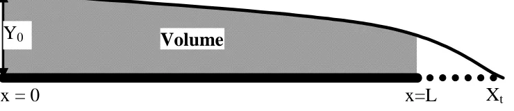
where σy is the shape factor for the advance phase, L is the length of the field and Xt is

an imaginary advance distance for the particular time, assuming that the advance can continue unimpeded past the end of the furrow (fig 1). This imaginary distance Xt is

calculated from the volume balance equation of the advance phase.

x=L

X

x = 0

Y

_Volume

Figure 1 Calculating the surface storage during the storage phase

In this case the volume stored in the furrow is:

L A

The cross sectional area Ao may be measured, predicted from the inflow using the

Manning equation, or calculated from a measured depth of flow. In the latter case the furrow geometry is presented as a power curve with provision for a flat bottom:

(13)

m B cy W

W = +

where W is the surface width of the flow, WB is the bottom width and y is the flow

depth. The parameters c and m are fitted by the model from measurements of the bottom, middle and top widths and maximum height of the furrow. Flow area is then simply calculated by integrating the flow width over the flow depth.

1 1 0 + + = + m cy y W A m o B

o (14)

As well as the measured advance (distances and times), the model requires measurements of the run-off volumes at various times during the storage phase. In field trials it is usual to measure the run-off hydrograph (run-off rate). The run-off volume at any particular time is calculated by the trapezoidal rule, assuming that the run-off hydrograph is linear between each run-off measurement.

The model attempts to minimize the difference between: (i) the calculated and measured advance distances during the advance phase, and (ii) the calculated and measured run-off volumes during the storage phase, by incrementing the parameters of the modified Kostiakov equation. The algorithms for each phase are:

∑

i z o i

a i z o y i o i advance t f kt A t Q x SSE 1 2 2 1 σ σ

σ (15)

(16)

(

)

[

]

∑

= Nr i o z a i z o ys i o Ri

runoff V Q t A L kt L f L SSE 1 2 2 1 σ σ σ

where SSE is the standard square error, xi, ti and VRi are the measured advance

distance, time and run-off volumes, respectively, Na is the number of advance points,

and Nr is the number of run-off volumes. Finally, the objective function is formed by

non-dimensionalising and summing the advance and run-off errors, weighted by a predetermined factor. 2 1 1 2 2 1 1 2 * _ ⎟ ⎟ ⎟ ⎟ ⎠ ⎞ ⎜ ⎜ ⎜ ⎜ ⎝ ⎛ + ⎟ ⎟ ⎟ ⎟ ⎠ ⎞ ⎜ ⎜ ⎜ ⎜ ⎝ ⎛ =

∑

∑

The weighting factor, w is included to enable the user to easily change the relative sensitivity of the objective function to the errors of the advance distance or runoff volume.

This objective function can also be expressed in terms of errors in both advance and runoff time. This results in parameter values very similar to those from equation 17 but requires further iterative computations as some of the terms in the model such as the subsurface shape factors (equations 7 and 8) are time dependant.

The optimisation scheme is based on the technique introduced by McClymont and Smith (1996); each of the three parameters (a, k and fo) is incremented individually

until the error reduces no further. Following this the parameters are incremented in the same direction as before but as a group until the error again cannot be reduced further. These two steps are repeated until the objective function is not improved by either the individual or group search. Now the step size is reduced and the whole process repeats.

During the design process it was noticed that occasionally the program jumped to the next smallest step size too quickly or remained incrementing at a particular step size for a long period of time. To overcome these problems the optimisation increases the group step size each time the program loops back to the individual parameter search.

The initial step sizes for the parameter optimisation are selected based on maximum stability combined with minimum execution time. The initial step sizes can be changed but experimentation has found 0.01, 0.0001 and 0.00001 for the step sizes of

a, k and f0 respectively work with most data sets.

Comprehensive tests were carried out to determine the sensitivity of the model to various inputs. These showed that the model is not significantly sensitive to furrow geometry but is influenced by other inputs such as the Manning constant.

parameter search. Also, limits have been included to ensure that the parameters do not reach unrealistic values (for example all three parameters are kept positive).

The model has been coded in C++ to create an executable program (IPARM); once it is loaded the user is required to enter input data.

The model requires a number of input measurements. Firstly the advance data in the form of distances and corresponding times, the technique requires a minimum of two advance points. Secondly the run-off data is made up of run-off rates (in l/s) measured at various times during the storage phase (the model is not valid during the depletion and recession phases). Other inputs include field slope, Manning n or upstream flow depth, inflow rate and the field length.

Model Verification

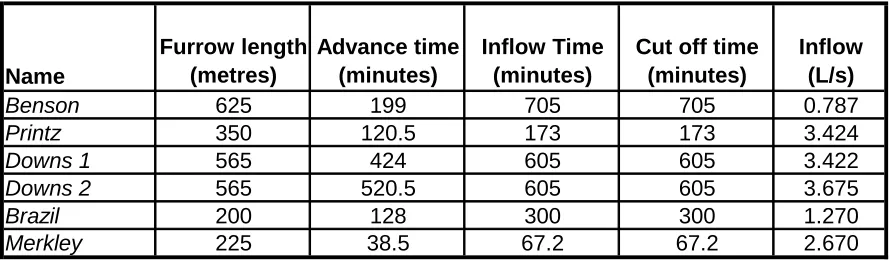
Trials of the model have been carried out using a number of data sets, six of which (Table 1) have been selected for discussion. The selected irrigations cover a wide range of soil types, flow rates and irrigation durations.

Table 1: Comparing the selected data sets

Name

Furrow length (metres)

Advance time (minutes)

Inflow Time (minutes)

Cut off time (minutes)

Inflow (L/s)

Benson 625 199 705 705 0.787

Printz 350 120.5 173 173 3.424

Downs 1 565 424 605 605 3.422

Downs 2 565 520.5 605 605 3.675

Brazil 200 128 300 300 1.270

Merkley 225 38.5 67.2 67.2 2.670

The Benson and Printz trials were carried out in Colorado on clay loam and sandy loam soils, respectively (Walker, 2005). The Benson case study is an example where the advance phase of the irrigation is relatively short compared to the storage phase.

(Dalton et al., 2001). The two data sets are titled Downs1 (Irrigation 2 furrow 3) and Downs2 (Irrigation 2 furrow 2).

The final two data sets, Brazil and Merkley, were sourced from Scaloppi et al. (1995). Both of these, in particular the Merkley trial are typical examples of where the advance data does not cover an adequate time to enable the accurate calculation of the infiltration function from the advance data alone.

Infiltration parameters were calculated for each irrigation using the maximum available number of both run-off and advance points for each data set. The optimisation was performed with equal weighting on both the advance and storage phases (see equation 17). To identify the improvement offered by of the proposed technique, the infiltration parameters were also calculated from advance data alone, with results similar to those produced by INFILT (McClymont and Smith, 1996). Values for the upstream flow area were calculated from estimates of Manning n and the furrow geometry.

The surface irrigation simulation model SIRMOD (Walker 1999) was then used to simulate the irrigation events using the different sets of infiltration parameters. In each case the values for a, k and fo were entered into the model and the value of the

Manning n was adjusted to cause the model to predict the end of the advance phase correctly. All simulations were performed by SIRMOD II using the full hydrodynamic model option. SIRMOD produces advance curves and run-off hydrographs that can be compared with the measured data. Other outputs include the total infiltration and total outflow.

Results and Discussion

Model Performance

The IPARM model was able to calculate infiltration functions for all of the case studies (Table 2). The values of the individual parameters a, k and fo vary

differences, the cumulative infiltration functions (fig 2.a-f) have similar shapes within each trial. In most cases the two infiltration curves indicate similar infiltrated volumes at times less than the end of the advance phase, in fact the curves cross at a time close to the advance time. The greatest difference between the curves is seen after the end of the advance phase where after the two curves diverge substantially. This difference or error will continue to increase if the curves are extrapolated to greater times. This has enormous implications if the infiltration parameters are to be used in the simulation or management of an irrigation at times greater than the advance time.

Table 2: Estimated Infiltration Parameters

a k f0

Advance 0 0.00163 0.000070

Advance + Runoff 0.4553 0.00058 0.000041

Advance 0 0.02624 0.000372

Advance + Runoff 0.0960 0.01539 0.000477

Advance 0 0.04731 0.000320

Advance + Runoff 0.2932 0.01889 0.000149

Advance 0 0.09316 0.000275

Advance + Runoff 0.1673 0.05037 0.000176

Advance 0.6831 0.00212 0.000000

Advance + Runoff 0.3354 0.00463 0.000263

Advance 0.5449 0.00284 0.000000

Advance + Runoff 0.2890 0.00264 0.000402

Trial Data Kostiakov Parameters

Benson

Merkley Printz

Downs 1

Downs 2

Brazil

0 0.01 0.02 0.03 0.04 0.05 0.06

0 20 40 60 80 100 120

Time (minutes) In filt ra ti o n ( m 3/m ) Advance Advance + Runoff 0 0.02 0.04 0.06 0.08 0.1 0.12 0.14

0 50 100 150 200 250 300 350 400

Time (minutes) In filt ra ti o n ( m 3/m ) Advance Advance + Runoff 0 0.05 0.1 0.15 0.2 0.25 0.3

0 100 200 300 400 500 600 700

Time (minutes) Inf iltratio n ( m 3/m) Advance Advance + Runoff

0 0.05 0.1 0.15 0.2 0.25 0.3

0 100 200 300 400 500 600 700 800

Time (minutes) Inf iltratio n ( m 3/m) Advance Advance + Runoff 0 0.02 0.04 0.06 0.08 0.1 0.12 0.14

0 50 100 150 200

Time (minutes) Inf il tra ti on (m ^3 /m ) Advance Advance + Runoff 0 0.01 0.02 0.03 0.04 0.05 0.06

0 100 200 300 400 500 600 700

Time (minutes) In fil tra ti on (m ^ 3 /m ) Advance Advance + Runoff

a

Benson

b

Prinz

c

Downs 1

d Downs 2 e Brazil f Merkley

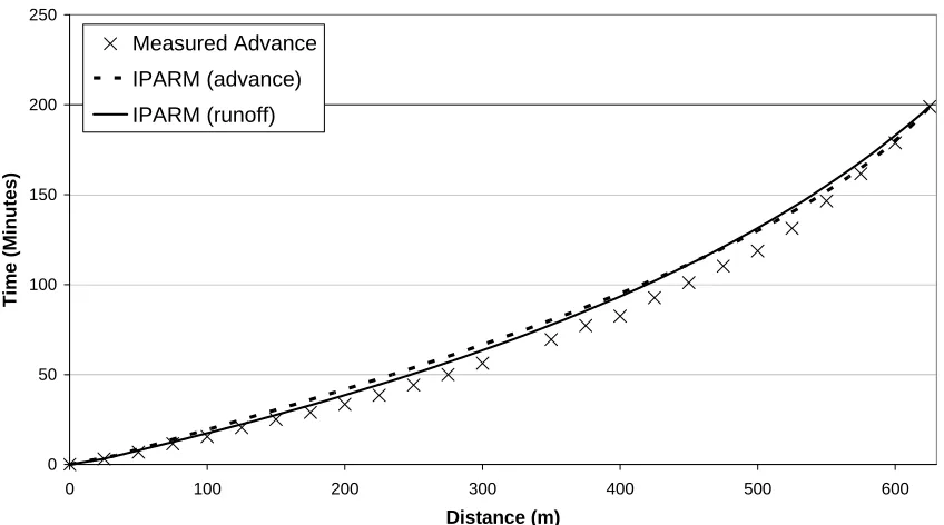
adjusting the value of Manning n. The resulting n values ranged between 0.016 and 0.05 reflecting realistic values. In each example the Manning n in SIRMOD more closely reflected the assumed value for the parameter optimisation where runoff data was used. The example in fig 3 demonstrates the typical behaviour found for all data sets studied. That is the inclusion of run-off data in the calculation of the infiltration parameters does not compromise the ability of the simulations to reproduce the advance data.

0 50 100 150 200 250

0 100 200 300 400 500 600

Distance (m)

Time (

M

inut

es

)

Measured Advance

IPARM (advance)

IPARM (runoff)

Figure 3 Comparing the measured advance curve of the Benson data with simulated advance curves.

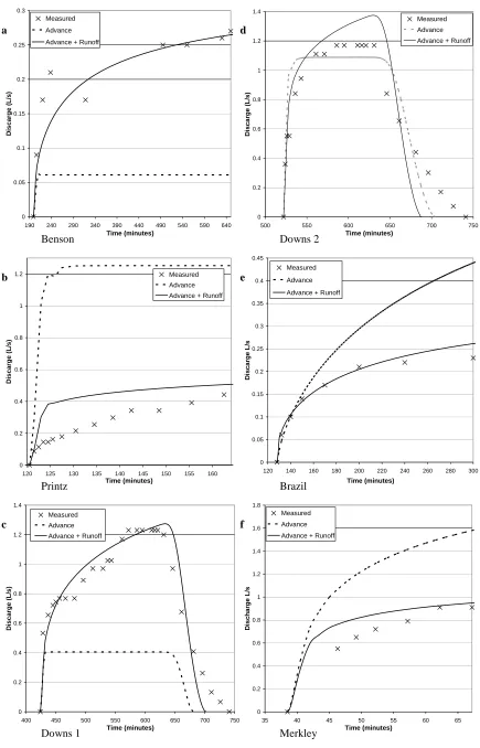
Any differences between the simulations caused by the different infiltration parameters become more apparent in a comparison of the predicted run-off hydrographs (fig 4). The results of the simulations show that in every case (perhaps with the slight exception of

0 0.2 0.4 0.6 0.8 1 1.2 1.4 1.6 1.8

35 40 45 50 55 60 65

Time (minutes) D isc h a rg e L /s Measured Advance Advance + Runoff

0 0.05 0.1 0.15 0.2 0.25 0.3 0.35 0.4 0.45

120 140 160 180 200 220 240 260 280 300

Time (minutes) Disca rge L /s Measured Advance Advance + Runoff

0 0.2 0.4 0.6 0.8 1 1.2 1.4

500 550 600 650 700 750

Time (minutes) Disca rge ( L /s) Measured Advance Advance + Runoff

0 0.2 0.4 0.6 0.8 1 1.2 1.4

400 450 500 550 600 650 700 750

Time (minutes)

Disc

arge (L/s)

Measured Advance Advance + Runoff

0 0.2 0.4 0.6 0.8 1 1.2

120 125 130 135 140 145 150 155 160

Time (minutes) Dis carge (L /s) Measured Advance Advance + Runoff

0 0.05 0.1 0.15 0.2 0.25 0.3

190 240 290 340 390 440 490 540 590 640

Time (minutes) D is carge (L /s) Measured Advance Advance + Runoff

a

Benson

b

Printz

c

Downs 1

d

Downs 2

e

Brazil

f

Merkley

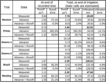
Table 3 Summary of results from SIRMOD simulations

Measured 5.84 7.76 26.89

Advance 1.63 -72.1% 2.13 -72.6% 32.81 22.0% Advance + Runoff 5.82 -0.3% 8.02 3.4% 26.61 -1.0%

Measured 0.74 1.64 62.91

Advance 3.01 305.3% 6.41 292.3% 54.05 -14.1% Advance + Runoff 1.10 48.6% 2.10 28.7% 62.04 -1.4%

Measured 15.13 96.55

Advance 5.72 -62.2% 104.87 8.6%

Advance + Runoff 15.44 2.0% 96.28 -0.3%

Measured 9.73 109.45

Advance 9.62 -1.1% 109.55 0.1%

Advance + Runoff 10.08 3.6% 109.14 -0.3%

Measured 1.97 2.30 128.51

Advance 3.06 55.2% 3.31 44.0% 122.19 -4.9% Advance + Runoff 2.08 5.2% 2.34 1.8% 128.25 -0.2%

Measured 1.11 2.20 47.60

Advance 2.05 84.1% 4.07 85.1% 37.22 -21.8% Advance + Runoff 1.35 21.1% 2.46 11.9% 46.15 -3.1%

Data

Downs 2

Brazil

Merkley Benson

Printz

Downs 1 Trial

Infiltration mm

Infiltration Error At end of

recorded time

Total, at end of irrigation (Italic cells are estimated) Runoff

(m3)

Runoff Error

Runoff (m3)

Runoff Error

Similarly, the error in the predicted run-off volumes is also significant (Table 3), for example, the run-off volume is over predicted by nearly 300% for the Printz irrigation, which corresponds to an under prediction of the average infiltrated depth by an estimated 14%.

In summary the inclusion of the run-off data in the identification of the modified Kostiakov parameters gives a greatly improved estimate of the parameters and hence improved cumulative infiltration curve. It retains the ability of the simulations to predict the advance function and it improves the accuracy of run-off and infiltration predictions during later stages of the irrigation.

Number of Run-off and Advance Points

this data there was a large difference between the infiltration functions calculated by the two methods.

Table 4: Advance data for Merkley

Distance (m) Time (min)

1 25

2 50

3 75

4 100 13.4

5 125 17.6

6 150 22.3

7 175 27.4

8 200 32

9 225 38.5

2.3 5.4 8.8

Table 5: Run-off data for Merkley Time (min) Outflow (L/s) 1 46.3

2 49.2 3 52.2 4 57.2 5 62.2 6 67.2

0.55 0.65 0.72 0.79 0.91 0.91

0 0.01 0.02 0.03 0.04 0.05 0.06 0.07 0.08 0.09 0.1

0 20 40 60 80 100 120 140

Time (minutes)

Infiltr

a

tion (m^3/m)

All advance (9 points) advance (2 4 6 8) advance (4 9) advance (1 2 3 4) runoff +advance (2 4 6 8) runoff + advance (4 9) runoff + advance (1 2 3 4) runoff + advance (all 9 points)

Figure 5 Comparing the two methods and their sensitivity to the correct selection of advance points

0 0.01 0.02 0.03 0.04 0.05 0.06 0.07 0.08

0 20 40 60 80 100 120 140

Time (minutes)

In

fi

ltr

a

ti

on

(m

^3/m

)

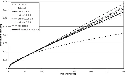
no runoff 1st point points 1 & 2 points 1,2 & 3 points 1,2,3 & 4 points 4,5 & 6 just point 6

all points 1,2,3,4,5 & 6

Figure 6 Impact of using different run-off points in the calculation of the infiltration function

better infiltration function than using no run-off data. Including the first two points is sufficient to provide an accurate estimation of the infiltration curve. When only the steady outflow rate is included, the model produces a poor answer indicating that the shape of the run-off hydrograph is important, not just the final outflow rate. There is little difference between using all six points and only the even numbered points indicating that the number of points is not important as long as the points used represent a significant portion of the storage phase.

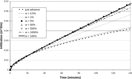
Weighting between Run-off and Advance Data

The weighing factor allows the user to change the relative importance of the advance and run-off data in the optimization of the infiltration function. It functions as a multiplier on the sum of errors in the predicted run-off volumes in equation 17. A value of 1 (100%) causes the relative error of the advance (equation 15) and the run-off (equation 16) to be of equal significance. The model will ignore the run-off if the weight is 0 and will ignore the advance data if the weight is given an extremely large value.

0 0.01 0.02 0.03 0.04 0.05 0.06 0.07

0 20 40 60 80 100 120 140

Time (minutes)

Infi

ltration

(m^3/m)

just advance w = 0.5% w = 1% w = 5% w = 50% w = 200% w = 1000% w = 100%

Figure 7 Effect of changing the weight of the run-off error in the Kostiakov parameter optimisation (100% is equal weight, <100% increases importance of the advance data)

Recommendations for the technique

The proposed parameter estimation procedure performed satisfactorily for the case studies presented here, however the volume balance model is based on a number of simplifications that may limit its application in certain conditions. The inflow rate throughout the entire irrigation should be constant with time as relatively small fluctuations may significantly impact on both the advance trajectory and runoff hydrograph. The model is only designed to apply during the storage phase therefore it is only valid to use runoff data collected during the inflow time. Further the location of the runoff measurement should be such that the measurement does not impose a backwater on the flow in the furrow.

Conclusions

infiltration parameters that cannot accurately predict run-off volumes. The use of run-off data enables the extrapolation of the infiltration curve to greater times, which is of particular importance where the advance reaches the end of the furrow early in the irrigation time.

References

Dalton, P., S. R. Raine and K. Broadfoot (2001). Best management practices for maximising whole farm irrigation

efficiency in the Australian cotton Industry. Final report to the Cotton Research and Development Corporation. National

Centre for Engineering in Agriculture Report. 179707/2, USQ, Toowoomba.

Elliott, R. L. and W. R. Walker (1982). "Field Evaulation of Furrow Infiltration and Advance Functions." Transactions

of the ASAE 25(2): 396-400.

Elliott, R. L., W. R. Walker and G. V. Skogerboe (1983). "Infiltration Parameters from Furrow Irrigation Advance

Data." Transactions of the ASAE 26(6): 1726-1731.

McClymont, D. J. and R. J. Smith (1996). "Infiltration parameters from optimization on furrow irrigation advance data."

Irrigation Science 17(1): 15-22.

Renault, D. and W. W. Wallender (1996). "Initial-inflow-variation impacts on furrow irrigation evaluation." Journal of

Irrigation and Drainage Engineering 122(1): 7-14.

Renault, D. and W. W. Wallender (1997). "Surface storage in Furrow irrigation evaluation." Journal of Irrigation and

Drainage Engineering 123(6): 415-422.

Scaloppi, E. J., G. P. Merkley and L. S. Willardson (1995). "Intake parameters from advance and wetting phases of

surface irrigation." Journal of Irrigation and Drainage Engineering 121(1): 57-70.

Walker, W. R. (1999). SIRMOD II Surface irrigation design, evaluation and simulation software--User's guide and

technical documentation, Utah State University, Logan, Utah.

Walker, W. R. (2005). "Multi-Level Calibration of Furrow Infiltration and Roughness." Journal of Irrigation and

Drainage Engineering 131(2):129-135.