two-dimensional steady-state heat conduction problems
.
White Rose Research Online URL for this paper:
http://eprints.whiterose.ac.uk/81061/
Version: Accepted Version
Article:
Karageorghis, A, Lesnic, D and Marin, L (2014) Regularized collocation Trefftz method for
void detection in two-dimensional steady-state heat conduction problems. Inverse
Problems in Science and Engineering, 22 (3). 395 - 418. ISSN 1741-5977
https://doi.org/10.1080/17415977.2013.788172
[email protected] https://eprints.whiterose.ac.uk/ Reuse
Unless indicated otherwise, fulltext items are protected by copyright with all rights reserved. The copyright exception in section 29 of the Copyright, Designs and Patents Act 1988 allows the making of a single copy solely for the purpose of non-commercial research or private study within the limits of fair dealing. The publisher or other rights-holder may allow further reproduction and re-use of this version - refer to the White Rose Research Online record for this item. Where records identify the publisher as the copyright holder, users can verify any specific terms of use on the publisher’s website.
Takedown
If you consider content in White Rose Research Online to be in breach of UK law, please notify us by
TWO-DIMENSIONAL STEADY-STATE HEAT CONDUCTION PROBLEMS
A. KARAGEORGHIS, D. LESNIC, AND L. MARIN
Abstract. We propose the use of the Trefftz collocation method for the solution of inverse geometric problems and, in particular, the determination of the boundary of a void. As was the case in the solution of such problems using the method of fundamental solutions, the algorithm for imaging the interior of the medium also makes use of radial polar parametrization of the unknown void shape in two dimensions. The centre of this radial polar parametrization is considered to be unknown. The feasibility of this new method is illustrated by several numerical examples highlighting its advantages and shortcomings.
1. Introduction
Numerous practical problems in engineering and sciences are characterised by the fact that one or more of the following conditions are partially or entirely unknown: the geometry of the domain of interest, the complete boundary and initial conditions, the material properties and the external sources acting in the solution domain. These problems are known asinverse problems and it are, in general, ill-posed [18], in the sense that the existence, uniqueness and stability of their solutions are not always guaranteed, and hence more difficult to solve. An important class of inverse problems is represented by the so-calledinverse geometric problems whose main feature is the lack of knowledge of part of the boundary. In particular, we focus herein on the numerical reconstruction of an internal boundary (i.e. cavity or rigid inclusion) in steady-state isotropic heat conduction (Laplace’s equation) from the knowledge of the temperature and normal heat flux (i.e. Cauchy data) on the outer boundary and an appropriate boundary condition for the unknown void.
The uniqueness of solution of the inverse geometric steady-state heat conduction problem related to the determi-nation of rigid inclusions or cavities from Cauchy data prescribed on the outer boundary of the solution domain for media with constant conductivity was proved in [19] and [48], respectively. The numerical reconstruction of voids in heat conduction problems has been tackled by numerous authors and various approaches have been proposed for the solution of this inverse geometric problem, see e.g. [1, 6, 13, 17, 27, 28, 32, 33, 34, 35, 46, 47, 53]. Das and Mitra [13] developed an iterative algorithm to determine the location and shape of a flaw in steady-state heat conduction (i.e. Laplace’s equation). Kassab and Pollard [32, 33] proposed a linear boundary element method (BEM), an anchored grid pattern method and a Newton-Raphson method with a Broyden update for the numerical reconstruction of an unknown cavity for the same inverse geometric heat conduction problem. The conjugate gradient method (CGM) for the numerical solution of inverse design problems in estimating the optimal locations and shapes of the internal cooling passages for turbine blades based on the desired outer surface temperature distribution was considered in [24]. Gallego and Suarez [17] proposed an approach based on a boundary integral equation for the variation of the potential and flux to retrieve numerically an assumed flaw in the case of a two-dimensional isotropic solid subject to thermal loads. An iterative algorithm based on a real coded geneatic algorithm (GA) and the BEM for detecting cavities in problems governed by the two-dimensional Laplace equation was developed in [46], while [6] proposed a simplification of the CGM for the reconstruction of voids in two-dimensional steady-state isotropic heat conduction which consists of prescribing the values of the step size for the optimal searches to be constant values
Date: November 5, 2012.
2000Mathematics Subject Classification. Primary 65N35; Secondary 65N21, 65N38.
Key words and phrases. Void detection, inverse problem, Trefftz method, collocation.
depending upon the resolution of the identification. An iterative algorithm using thermographic techniques based on the superposition of clusters of sources/sinks with the BEM [34] was employed for the detection of subsurface cavities and flaws. Mera [47] used kriging approximation models to speed-up the optimization process via GAs for detecting the size and location of subsurface cavities associated with the two-dimensional Laplace’s equation, whilst Tan et al. [50] solved a geometry identification problem in two-dimensional isotropic heat conduction by employing the least-squares collocation meshless method and CGM. Kazemzadeh-Parsi and Daneshmand [35] approached the cavity detection problem for the two-dimensional Laplace equation via the smoothed fixed grid finite element method in conjunction with the CGM. Yan and Ma [53] considered the reconstruction of a cavity in the case of the Laplace equation from the knowledge of the measurements on the exterior boundary and employed the domain derivative of the associated operator and a regularized Newton method for the solution of the corresponding ill-posed and nonlinear problem. Recently, Karageorghis and Lesnic [27] proill-posed a method of fundamental solution (MFS)-based reconstruction of a cavity for the two-dimensional stationary heat conduction equation in isotropic media, whereas Borman et al. [1] and Karageorghis and Lesnic [28] employed the same approach for the detection of inclusions.
Trefftz methods [51] have been used extensively for the solution of elliptic boundary value problems, see, for example [38, 39, 52], and also [55]. Surveys on Trefftz and related methods may be found in [26, 36, 40, 55]. In this work we investigate the performance of the Trefftz collocation method (TCM) for the solution of inverse geometric problems, in particular for void detection problems. The TCM is a boundary meshless method and such methods have, in recent years, become increasingly popular for the solution of inverse problems in general because of the ease with which they can be implemented for boundary value problems in complex geometries and in three dimensions. The MFS in particular has been used extensively for the solution of inverse problems [30]. Trefftz methods have been used for the solution of inverse Cauchy linear problems [7, 8, 9, 10, 31, 43, 54]. In the case of inverse geometric problems the TCM has been recently used by Fan and his co-workers [3, 14, 15]. In particular, [15] deals entirely with boundary identification problems for Laplace’s equation, while in [3] an internal void problem is solved in the case of the Helmholtz equation. The ideas developed in this work are close to the ones developed in [14], see also [2], where two internal void detection problems are solved in the case of the Laplace equation. However, our proposed algorithm differs from the one in [14] as follows:
• In contrast to the algorithm of [14] for void detection inverse problems, we consider problems in which the centre(s) of the void(s) to be reconstructed is (are) unknown. The coordinates of the centre(s) are merely taken as additional unknowns in the algorithm.
• By changing and augmenting the Trefftz basis, the algorithm is capable of locating multiple inclusion with unknown centres.
• Instead of using a scalar homotopy algorithm we use the state-of-the-art MATLAB optimization toolbox routinelsqnonlin. This routine allows for the imposition of simple bounds on the variable which, to a great extent, eliminates physically unrealistic solutions.
• The stability of the proposed algorithm is achieved using two regularization parameters which can be determined by the use of the L-curve criterion. The method is shown to accurately reconstruct smooth or piecewise smooth, convex or concave, single or multiple cavities and rigid inclusions.
• We are not using the so-called modified collocation Trefftz method of [41, 42] which takes into account the characteristic shapes of the domains involved. This is because the size of at least one of the domains in unknown and needs to be determined as part of the solution. Efforts to normalize one set of unknowns produced little or no difference to our results.
a degenerate situation of the MFS with the source points placed at infinity. The corresponding result in annular and exterior domains may be found in [4] and [49], respectively.
2. Mathematical formulation
In this section we formulate the direct and inverse problems related to a void such as a rigid inclusion or a cavity in the case of steady-state heat conduction (Laplace’s equation). The direct problem given by the Laplace equation
∆u = 0 in Ω, (2.1a)
subject to the Dirichlet boundary condition
u = f on ∂Ω2, (2.1b)
and the homogeneous boundary condition
αu+ (1−α)∂nu = 0 on ∂Ω1, where α∈ {0,1}, (2.1c) has a unique weak solutionu∈ H1(Ω)iff ∈ H1/2(∂Ω
2), and a unique classical solutionu∈ C2(Ω)∩ C( ¯Ω), provided
f is sufficiently smooth. In the above,Ω = Ω2\Ω1, whereΩ1⊂Ω2, is a bounded annular domain with boundary
∂Ω =∂Ω1∪∂Ω2 and we assume thatΩis connected. Equation (2.1c), covers both Dirichlet (α= 1), i.e. a rigid inclusion, and Neumann (α= 0), i.e. a cavity, boundary conditions on∂Ω1.
The inverse problem we are concerned with consists of determining not only the functionu, but also the void Ω1 so that usatisfies the Laplace equation (2.1a), given the Dirichlet dataf ̸≡constant in (2.1b), the homogeneous boundary condition (2.1c) and the Neumann current flux measurement
g := ∂nu on ∂Ω2. (2.1d)
In (2.1c) and (2.1d), the vectorndenotes the outward unit normal to the annular domainΩ. Whenα= 0, for (2.1a), (2.1c) and (2.1d) to be consistent, we require
∫
∂Ω2
g(s)ds= 0. (2.2)
In contrast to the direct (forward) boundary value problem (2.1a)-(2.1c), the inverse problem (2.1a)-(2.1d) is nonlinear and ill-posed. Although the solution is unique, [19], it is unstable with respect to small errors in the input Cauchy data (2.1b) and (2.1d).
3. Trefftz collocation method
In the TCM for the doubly-connected two-dimensional annular domainΩ, we seek an approximation to the solution of Laplace’s equation (2.1a) as a linear combination of T-complete functions in the form [42, 22, 23]
uN(α,β,γ,δ;x) =α0+γ0log|z|+
N ∑
k=1
αkℜ{zk}+ N ∑
k=1
βkℑ{zk}
+
N ∑
k=1
ckℜ{z−k}+ N ∑
k=1
dkℑ{z−k}, x= (x, y)∈Ω, (3.1)
where the T-complete system is given by
{
1,log|z|,ℜ(zn),ℑ(zk),ℜ(z−k),ℑ(z−k);z=x+iy, k∈N}
, (3.2)
where ℜand ℑ denote the real and imaginary part of a complex number, respectively. In (3.1), there are 4N+ 2 unknowns, namely the coefficients α = [α0, α1, . . . , αN]T, β = [β1, β2, . . . , βN]T, γ = [γ0, γ1, . . . , γN]T, δ =
Without loss of generality, we shall assume that the (known) fixed exterior boundary ∂Ω2 is a circle of radiusR. As a result, the outer boundary collocation points are chosen as
xM1+ℓ=R(cos ˜ϑℓ,sin ˜ϑℓ), ℓ= 1, M2, (3.3)
whereϑ˜ℓ= 2πM(ℓ−21), ℓ= 1, M2.
We further assume that the unknown boundary∂Ω1is a smooth, star-like curve with respect to the centre which has unknown coordinates(X, Y). This means that its equation in polar coordinates can be written as
x=X+r(ϑ) cosϑ, y=Y +r(ϑ) sinϑ, ϑ∈[0,2π), (3.4) whereris a smooth 2π−periodic function. The constraint thatΩ1⊂Ω2 then recasts as
(X+r(ϑ) cosϑ)2+ (Y +r(ϑ) sinϑ)2< R2, ϑ∈[0,2π). (3.5) The discretized form of (3.4) for∂Ω1 becomes
rk=r(ϑk), k= 1, M1 (3.6) and we choose the inner boundary collocation points as
xk = (X, Y) +rk(cosϑk,sinϑk), (3.7)
whereϑk =2π(Mk−11), k= 1, M1.
Since the centre is not known and therefore not necessarily the origin, the basis (3.2) needs to be modified to
{
1,log|z−z0|,ℜ(zn),ℑ(zn),ℜ((z−z0)−n),ℑ((z−z0)−n);z=x+iy, n∈N}, (3.8) where z0 = X +iY. For example, this is suggested by function theoretic results concerning the expansion of functions that are analytic in multiply-connected domains [16, page 244], see also [37]. Therefore, the TCM approximation becomes
uN(α,β,γ,δ;x) =α0+γ0log|z−z0|+
N ∑
k=1
αkℜ{zk}+ N ∑
k=1
βkℑ{zk}
+
N ∑
k=1
γkℜ{(z−z0)−k}+
N ∑
k=1
δkℑ{(z−z0)−k}, x= (x, y)∈Ω. (3.9) In the cases where R >1 we tried to scale the terms in the first and second series in (3.9) through division with
Rk as suggested by Liu [41, 42]. This produced little or no improvement to our results. This may be because the
corresponding multiplication of each of the terms in the third and fourth series in (3.9) by Rk
c, whereRc is the
characteristic length of∂Ω1, as suggested in [42] is not possible as its size is unknown.
4. Implementational details
The current flux data (2.1d) come from practical measurements which is inherently contaminated with errors due to noise, and we therefore replaceg by the noisy datagεdefined as
gε(xj) = (1 +ρjp)g(xj), j=M1+ 1, M1+M2, (4.1) whereprepresents the percentage of noise andρj is a pseudo-random noisy variable drawn from a uniform
The coefficients (ak)k=0,N,(bk)k=0,N,(ck)k=1,N and (dk)k=1,N in (3.1), the radii (rk)k=1,M1 in (3.6), and the
coordinates of the centre C = (X, Y) are determined by imposing the boundary conditions (2.1b), (2.1c) and (2.1d) in a least-squares sense. This leads to the minimization of the functional
S(α,β,γ,δ,r,C) : =
M1+M2
∑
j=M1+1
[uN(α,β,γ,δ;xj)−f(xj)]2+ M1+M2
∑
j=M1+1
[∂nuN(α,β,γ,δ;xj)−gε(xj)]2
+
M1
∑
j=1
[αuN(α,β,γ,δ;xj) + (1−α)∂nuN(α,β,γ,δ;xj)]2
+λ1(|α|2+|β|2+|γ|2+|δ|2)+λ2
M1
∑
ℓ=2
(rℓ−rℓ−1)2, (4.2) whereλ1, λ2≥0are regularization parameters to be prescribed.
In (4.2), the outward normal vectornis defined as follows:
n=
cosϑi+ sinϑj, if x∈∂Ω2,
1
√
r2(ϑ) +r′2(ϑ)
[−(r′(ϑ) sinϑ+r(ϑ) cosϑ)i+ (r′(ϑ) cosϑ−r(ϑ) sinϑ)j], if x∈∂Ω
1, (4.3) wherei= (1,0)andj = (0,1). As a result, from (3.9) the normal derivative∂nuN is evaluated as
∂nuN =n· ∇uN =
n·
(
γ0
ℜ {z−z0}
|z−z0|2 +
N ∑
k=1
αkℜ{kzk−1}+ N ∑
k=1
βkℑ{kzk−1}
+
N ∑
k=1
γkℜ{−k(z−z0)−k−1}+
N ∑
k=1
δkℑ{−k(z−z0)−k−1},
γ0
ℑ {z−z0}
|z−z0|2
+
N ∑
k=1
αkℜ{ikzk−1}+ N ∑
k=1
βkℑ{ikzk−1}
+
N ∑
k=1
γkℜ {
−ki(z−z0)−k−1
}
+
N ∑
k=1
δkℑ {
−ki(z−z0)−k−1
} )
. (4.4)
In (4.3), we use the central finite-difference approximation
r′(ϑ
i)≈
ri+1−ri−1
4π/M1
, i= 1, M1, (4.5)
with the convention thatrN+1=r1, r0=rM1.
Since the total number of unknowns is4N+2+M1+2and the number of boundary condition collocation equations isM1+ 2M2 we need to take M2≥2N+ 2.
4.1. Non-linear minimization. The minimization of functional (4.2) is carried out using theMATLAB [45] opti-mization toolbox routine lsqnonlinwhich solves nonlinear least squares problems. This routine by default uses the so-called trust-region-reflective algorithm based on the interior-reflective Newton method [11, 12]. In addition,
lsqnonlin does not require the user to provide the gradient and, in addition, it offers the option of imposing lower and upper bounds on the elements of the vector of unknowns. Further details regarding the application of
5. Numerical examples
5.1. Example 1. We first consider an example from the literature for which the exact solution is known [1]. Here we examine the case of a circular rigid inclusion whereα= 1. In particular, we consider
Ω1=
{
(x, y)∈R2:x2+y2< R20<1}, Ω2={(x, y)∈R2:x2+y2< R2= 1} (5.1)
and
u(x, y) = log
√
x2+y2
R0
. (5.2)
For any0< R0<1, the functionusatisfies problem (2.1a)-(2.1d), with
f(x, y) =−logR0, g(x, y) = 1, (x, y)∈∂Ω2. (5.3) In our numerical experiments we consider the caseR0= 0.5. We take as initial guessesr0=0.3,a0=b0=0and
c0=d0
=0, and we fix as known the centreC at the origin(0,0).
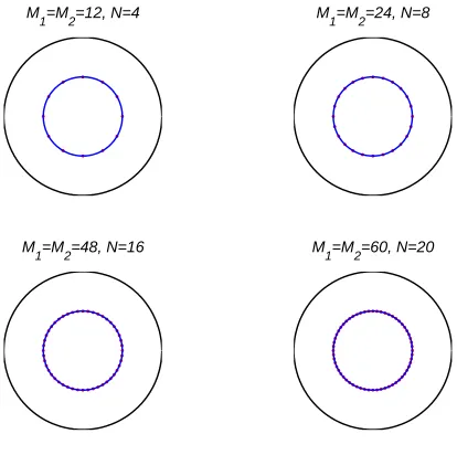
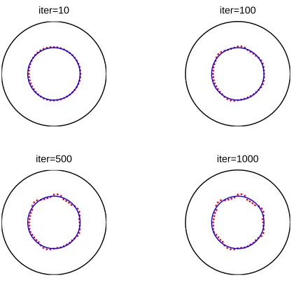
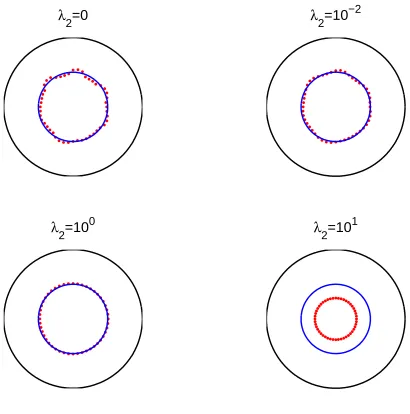
In Figure 1 we present the reconstructed curves for various numbers of degrees of freedom obtained in 20 iterations, no noise and no regularization. From this figure it can be seen that very accurate and convergent numerical results are obtained. In Figure 2 we present typical examples of reconstructed curves with noise level of p= 10%with no regularization and M1 =M2 = 48, N = 8 for different numbers of iterations. From this figure it can be seen that as the number of iterations increases instabilities start to manifest if no regularization is included. In Figure 3 we present the corresponding reconstructed curves with p= 10%, after 1000 iterations and various regularization parameters λ1 with λ2 = 0. The corresponding curves for various regularization parametersλ2 with λ1 = 0are presented in Figure 4. In some instances, in this and subsequent examples, the use of regularization leads the iterative process to converge in fewer than the prescribed maximum number of iterations. Overall from Figures 3 and 4 it can be seen that regularization with eitherλ1= 120 or λ2 = 1, respectively, does smooth out the slight oscillations recorded in the results of Figure 2 obtained after 1000 iterations with no regularization.
M
1=M2=12, N=4 M1=M2=24, N=8
M
[image:7.612.211.418.417.623.2]1=M2=48, N=16 M1=M2=60, N=20
Figure 1. Example 1: Results after 20 iteration for various numbers of degrees of freedom, no
iter=10 iter=100
[image:8.612.210.420.109.316.2]iter=500 iter=1000
Figure 2. Example 1: Results for noisep= 10%, no regularization and various numbers of iterations.
λ1=0 λ
1=10 1
λ1=102 λ
1=120
Figure 3. Example 1: Results after 1000 iterations for noisep= 10%and regularization withλ1.
5.2. Example 2. In this example, we consider a more complicated peanut-shaped rigid inclusion whose boundary
∂Ω1is described by the radial parametrization
r(ϑ) =3 4
√
[image:8.612.209.420.377.585.2]λ2=0 λ
2=10 −2
λ2=100 λ
[image:9.612.212.417.111.318.2]2=10 1
Figure 4. Example 1: Results after 1000 iterations for noisep= 10%and regularization withλ2.
in the case ofα= 1, which was considered in [25]. The Dirichlet data (2.1b) on∂Ω2is taken as [25]
u(1, ϑ) =f(ϑ) = e−cos2
ϑ, ϑ∈[0,2π). (5.5)
Since in this case no analytical solution is available, the Neumann data (2.1d) is simulated by solving the direct well-posed problem (2.1a), (2.1c) and (5.5), when∂Ω1is given by (5.4), using the direct TCM withM1=M2= 100, N=
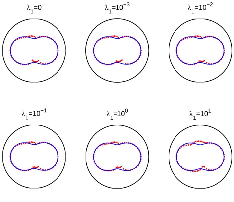
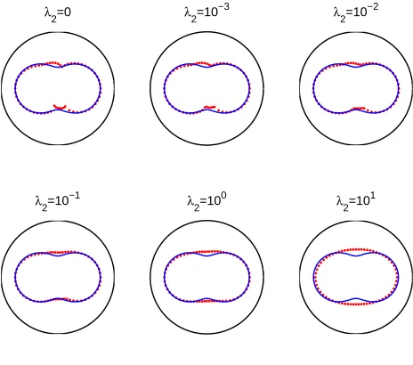
30. In order to avoid committing an inverse crime, the inverse solver is applied usingM1=M2= 64, N = 6. In Figure 5 we present typical examples of reconstructed curves with noise p = 10% with no regularization for different numbers of iterations. In Figures 6 and 7 we present the corresponding reconstructed curves withp= 10%, after 1000 iterations and various regularization parametersλ1 withλ2= 0, andλ2 withλ1= 0, respectively. The L-curves [21, 20] obtained with regularization inλ1 or λ2 for noisep= 10%and 1000 iterations are presented in Figures 8(a) and (b), respectively. From Figure 5 it can be seen that the numerically retrieved shapes are stable and in reasonable agreement with the exact shape (5.4). This is somewhat surprising since no regularization has been imposed, but it may be that oscillations will start to appear only after a larger number of iterations than 1000. Furthermore, Figure 6 shows that regularization with λ1 produces almost no improvement and, in fact, Figure 8(a) illustrates that an L-curve could not be obtained in this case. On the other hand, Figure 7 shows that regularization withλ2 between10−2to 1 does produce smoother and more stable and accurate solutions with the choice of the regularization parameter given by the corner of the L-curve illustrated in Figure 8(b).
5.3. Example 3. In this example, we again consider the peanut-shaped cavity whose boundary∂Ω1 is described by the radial parametrization (5.4), this time in the case of α= 0, which was studied in [25, 29]. As in Example 2, the Dirichlet data (2.1b) on∂Ω2 is given by (5.5). The Neumann data (2.1d) is simulated by solving the direct problem using the direct TCM with,M1=M2= 100, N= 28. In order to avoid committing an inverse crime, the inverse solver is applied usingM1=M2= 64, N= 5.
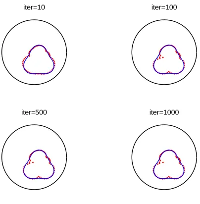
In Figure 9 we present typical examples of reconstructed curves with noise level ofp= 5%with no regularization for different numbers of iterations. In Figures 10 and 11 we present the corresponding reconstructed curves with
iter=10 iter=100
[image:10.612.210.419.109.317.2]iter=500 iter=1000
Figure 5. Example 2: Results for noisep= 10%, no regularization and various numbers of iterations.
λ1=0 λ
1=10
−3 λ
1=10 −2
λ1=10−1 λ
1=10
0 λ
1=10 1
Figure 6. Example 2: Results after 1000 iterations for noisep= 10%and regularization withλ1.
[image:10.612.196.432.373.576.2]λ2=0 λ
2=10
−3 λ
2=10 −2
λ2=10−1 λ
2=10
0 λ
[image:11.612.198.430.112.317.2]2=10 1
Figure 7. Example 2: Results after 1000 iterations for noisep= 10%and regularization withλ2.
0.5 0.75 1
1.35 1.4 100
[image:11.612.168.435.384.594.2]10−1
||Residual||
2
||
coefficients
||2
(a)
0.5 0.6 0.7
0.1 0.15 0.2
100
10−1
||Residual||2
||
r
′||2
(b)
Figure 8. Example 2: L-curves obtained with regularization in (a)λ1 and (b)λ2for noise p= 10%.
5.4. Example 4. We consider a rigid inclusion Ω1, i.e. α= 1, described by X = 0.5, Y =−1, R= 3.5 and the radial parametrization
iter=10 iter=100
[image:12.612.210.419.110.316.2]iter=200 iter=500
Figure 9. Example 3: Results for noisep= 5%and no regularization.
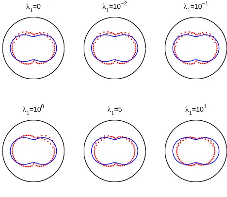
λ1=0 λ
1=10
−2 λ
1=10 −1
λ1=100 λ
1=5 λ1=10 1
Figure 10. Example 3: Results for noise p= 5%and regularization withλ1.
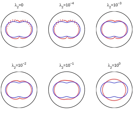
[image:12.612.196.430.383.586.2]λ2=0 λ
2=10
−4 λ
2=10 −3
λ2=10−2 λ
2=10
−1 λ
[image:13.612.197.431.110.312.2]2=10 0
Figure 11. Example 3: Results for noise p= 5%and regularization withλ2.
collocation points. The inverse TCM solver is applied using M1 =M2 = 64, N = 6. The starting position of the centre in the iterative process was taken to be the origin.
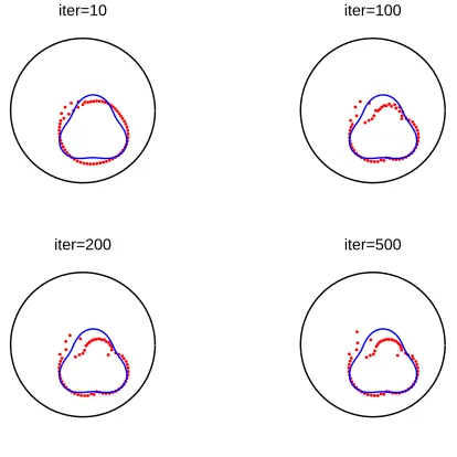
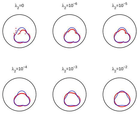
In Figure 12 we present typical examples of reconstructed curves with noise level ofp= 5%with no regularization for different numbers of iterations. In Figures 13 and 14 we present the corresponding reconstructed curves with
p= 5%, after 1000 iterations and various regularization parametersλ1withλ2= 0, andλ2withλ1= 0, respectively. From Figures 12-14, the same conclusions as those drawn from Figures 5-7 for Example 2 and Figures 9-11 for Example 3 are obtained. This shows that the reconstruction method also performs well when the centre of the star-shaped void is unknown.
5.5. Example 5. We finally consider the same obstacle as in Example 4, given by (5.6) but in the case ofα= 0, i.e. Ω1is a cavity. The numerical details are the same as in Example 4.
In Figure 15 we present the results obtained for different numbers of iterations, with p = 5% noise and no regularization. In Figures 16 and 17 we present the corresponding reconstructed curves with p = 5%, after 500 iterations and various regularization parametersλ1 withλ2 = 0, andλ2 withλ1= 0, respectively. From Figures 15 and 16 it can be seen that the numerically obtained shapes withλ1=λ2 = 0, orλ2 = 0,λ1>0, are unstable, whilst from Figure 17 it can be observed that regularization withλ2 between 10−4 and 10−2 produces smoother stable reconstructions.
6. Extension to multiple voids
The TCM analysis performed so far showed the successful implementation of this method for the identification of a single void. In this section we extend the analysis to multiple voids which may contain both cavities and rigid inclusions. For the sake of clarity, we describe the formulation for the case of two voids. Therefore, we consider the inverse problem
iter=10 iter=100
[image:14.612.214.416.109.315.2]iter=500 iter=1000
Figure 12. Example 4: Results for noisep= 5%, no regularization and various numbers of iterations.
λ1=0 λ1=10−6 λ1=10−5
λ1=10−4 λ1=10−3 λ1=10−2
Figure 13. Example 4: Results after 1000 iterations for noisep= 5%and regularization withλ1.
subject to the boundary conditions
u = f and ∂nu=g on ∂Ω2, (6.1b)
and the homogeneous boundary conditions
[image:14.612.200.429.374.569.2]λ2=0 λ
2=10
−4 λ
2=10 −3
λ2=10−2 λ
2=10
−1 λ
[image:15.612.202.425.112.310.2]2=10 0
Figure 14. Example 4: Results after 1000 iterations for noisep= 5%and regularization withλ2.
iter=10 iter=100
iter=200 iter=500
Figure 15. Example 5: Results for noisep= 5%, no regularization and various numbers of iterations.
and
[image:15.612.211.418.378.585.2]λ1=0 λ
1=10
−7 λ
1=10 −6
λ1=10−5 λ
1=10
−4 λ
[image:16.612.200.428.108.307.2]1=10 −3
Figure 16. Example 5: Results after 500 iterations for noisep= 5%and regularization withλ1.
λ2=0 λ
2=10
−6 λ
2=10 −5
λ2=10−4 λ
2=10
−3 λ
2=10 −2
Figure 17. Example 5: Results after 500 iterations for noisep= 5%and regularization withλ2.
The outer boundary collocation points are chosen as
xM1+M2+ℓ=R(cos ˜ϑℓ,sin ˜ϑℓ), ℓ= 1, M3, (6.2)
[image:16.612.198.427.374.575.2]We further assume that the unknown boundaries∂Ωa
1 and∂Ωb1 are a smooth, star-like curves with respect to their centres which haveunknowncoordinates (Xa, Ya)and (Xb, Yb), respectively. This means that their equations in
polar coordinates can be written as
x=Xa+ra(ϑ) cosϑ, y=Ya+ra(ϑ) sinϑ, (6.3)
x=Xb+rb(ϑ) cosϑ, y=Yb+rb(ϑ) sinϑ, ϑ∈[0,2π), (6.4) wherera andrb are smooth2π−periodic functions.
The discretized forms of (6.3) and (6.4) for∂Ωa
1 and∂Ωb1become
rak =ra(ϑk), k= 1, M1 and rbℓ=rb(ϑℓ) ℓ= 1, M2. (6.5) We choose the inner boundary collocation points as
xk = (Xa, Ya) +rka(cosϑk,sinϑk), k= 1, M1 (6.6)
xk = (Xb, Ya) +rkb(cosϑk,sinϑk), k=M1+ 1, M1+M2. (6.7) Since we have more than one void and their centres are not at the origin, the basis (3.2) needs to be modified as in the doubly connected domain, to (see [16])
{
1,log|z−za|,log|z−zb|,ℜ(zn),ℑ(zn),ℜ((z−za)−n),ℑ((z−za)−n),
ℜ((z−zb)−n),ℑ((z−zb)−n);z=x+iy, n∈N}
, (6.8)
whereza=Xa+iYa, zb=Xb+iYb and therefore the TCM approximation becomes
uN(α,β,γa,γb,δa,δb;x) =α0+γ0alog|z−za|+γ0blog|z−zb|+
N ∑
k=1
αkℜ{zk}+ N ∑
k=1
βkℑ{zk}
+ N ∑ k=1 γa kℜ {
(z−za)−k}
+ N ∑ k=1 δa kℑ {
(z−za)−k}
+ N ∑ k=1 γb kℜ {
(z−zb)−k}
+ N ∑ k=1 δb kℑ {
(z−zb)−k}
, (6.9) forx= (x, y)∈Ω.
The coefficients(αk)k=0,N,(βk)k=1,N,(γkℓ )
k=0,N ,ℓ=a,b, (
δℓ k )
k=1,N ,ℓ=a,bin (6.9), the radii(r a
k)k=1,M1,
(
rb k )
k=1,M2 in
(6.5), and the coordinates of the centres(Xa, Ya),(Xb, Yb)can be determined by imposing the boundary conditions
in a least-squares sense. This leads to the minimization of the functional
S(α,β,γa,γb,δa,δb,ra,rb,C) :=
M1+M2+M3
∑
j=M1+M2+1
[
uN(α,β,γa,γb,δa,δb;xj)−f(xj) ]2
+
M1+M2+M3
∑
j=M1+M2+1
[
∂nuN(α,β,γa,γb,δa,δb;xj)−gε(xj) ]2 + M1 ∑ j=1 [
α1uN(α,β,γa,γb,δa,δb;xj) + (1−α1)∂nuN(α,β,γa,γb,δa,δb;xj) ]2
+
M1+M2
∑
j=M1+1
[
α2uN(α,β,γa,γb,δa,δb;xj) + (1−α2)∂nuN(α,β,γa,γb,δa,δb;xj) ]2
+λ1
(
|α|2+|β|2+|γa|2+|γb|2+|δa|2+|δb|2)+λa
2 M1 ∑ ℓ=2 ( ra ℓ −raℓ−1
)2
+λb
2 M2 ∑ ℓ=2 ( rb ℓ−rbℓ−1
)2
, (6.10) where λ1, λa2, λb2≥0are regularization parameters to be prescribed, ra = [ra1, ra2, . . . , rNa]T, rb = [r1b, r2b, . . . , rbN]T,
and C = [Xa, Ya, Xb, Yb]T. The number of unknowns is 6N+ 3 +M
6.1. Example 6. We consider the case when two rigid inclusions α1 = α2 = 1) Ωa1 and Ωb1 are present. The domain Ωa
1 is a disk of radius 1, with centre Xa = 1, Ya = −1, while the domain Ωb1 is described by the radial parametrization
r(ϑ) = 1 + 0.8 cos(ϑ) + 0.2 sin(2ϑ)
1 + 0.7 cos(ϑ) , ϑ∈[0,2π), (6.11)
and has centreXb =−1, Yb= 1. In this example which was also examined in [29] we takeR= 3.5. The Neumann
data (2.1d) is simulated by solving the direct problem using the MFS with 600 singularities and 600 collocation points. The inverse TCM solver is applied using M1 =M2 = 32, M3 = 64, N = 6. The starting position of the centres in the iterative process was taken to be (0.5,-0.5) and (-0.5,0.5), respectively.
In Figure 18 we present the results obtained for different numbers of iterations, no regularization, andp= 5%noise. In Figures 19 and 20 we present the corresponding reconstructed curves with p= 5%noise, after 500 iterations, and various levels of regularizationλ1withλ2=λa2=λb2= 0, andλ1= 0withλ2=λa2=λb2, respectively. Overall, Figures 18-20 illustrate that the MFS can successfully retrieve voids having two connected components.
iter=10 iter=100
[image:18.612.214.418.293.498.2]iter=200 iter=500
Figure 18. Example 6: Results for noisep= 5%, no regularization and various numbers of iterations.
7. Conclusions
λ1=0 λ
1=10
−6 λ
1=10 −5
λ1=10−4 λ
1=10
−3 λ
[image:19.612.202.425.112.312.2]1=10 −2
Figure 19. Example 6: Results after 500 iterations for noisep= 5%and regularization withλ1.
λ2=0 λ2=10−5 λ2=10−4
λ2=10−3 λ2=10−2 λ2=10−1
Figure 20. Example 6: Results after 500 iterations for noisep= 5%and regularization withλ2.
[image:19.612.199.428.378.578.2]Acknowledgements
The authors wish to thank Professor Nick Papamichael for many enlightening discussions and are also grateful to the University of Cyprus for supporting this research. L. Marin also acknowledges the financial support received form the Romanian National Authority for Scientific Research, CNCS–UEFISCDI, project number PN–II–ID– PCE–2011–3–0521.
References
[1] D. Borman, D. B. Ingham, B. T. Johansson, and D. Lesnic,The method of fundamental solutions for detection of cavities in EIT, J. Integral Equations Appl.21(2009), 381–404.
[2] H.-F. Chan,Meshless Method and Exponentially Convergent Scalar Homotopy Algorithm for the Inverse Boundary Determination Problem, Master’s thesis, Department of Harbor and River Engineering, National Taiwan Ocean University, Keelung, Taiwan, 2011. [3] H.-F. Chan, C.-M. Fan, and W. Yeih, Solution of inverse boundary optimization problem by Trefftz method and exponentially
convergent scalar homotopy algorithm, CMC Comput. Mater. Continua24(2011), 125–142.
[4] J.-T. Chen, Y.-T. Lee, S.-R. Yu, and S.-C. Shieh,Equivalence between the Trefftz method and the method of fundamental solution for the annular Green’s function using the addition theorem and image concept, Eng. Anal. Bound. Elem.33(2009), 678–688. [5] J.-T. Chen, C.-S. Wu, Y.-T. Lee, and K.-H. Chen,On the equivalence of the Trefftz method and method of fundamental solutions
for Laplace and biharmonic equations, Comput. Math. Appl.53(2007), 851–879.
[6] C.-H. Cheng and M.-H. Chang,A simplified conjugate-gradient method for shape identification based on thermal data, Num. Heat Transfer, Part B43(2003), 489–507.
[7] M. Ciałkowski and K. Grysa,Trefftz method in solving the inverse problems, J. Inverse Ill-Posed Probl.18(2010), 595–616. [8] M. J. Ciałkowski and Fr¸ackowiak,Solution of the stationary 2D inverse heat conduction problem by Treffetz method, J. Thermal
Science11(2002), 148–162.
[9] M. J. Ciałkowski, A. Fr¸ackowiak, and K. Grysa, Physical regularization for inverse problems of stationary heat conduction, J. Inverse Ill-Posed Probl.15(2007), 347–364.
[10] ,Solution of a stationary inverse heat conduction problem by means of Trefftz non-continuous method, Int. J. Heat Mass Transfer50(2007), 2170–2181.
[11] T. F. Coleman and Y. Li,On the convergence of interior-reflective Newton methods for nonlinear minimization subject to bounds, Math. Programming67(1994), 189–224.
[12] ,An interior trust region approach for nonlinear minimization subject to bounds, SIAM J. Optim.6(1996), 418–445. [13] S. Das and A. K. Mitra,An algorithm for the solution of inverse Laplace problems and its application in flaw identification in
materials, J. Comput. Phys.99(1992), 99–105.
[14] C.-M. Fan and H.-F. Chan,Modified collocation Trefftz method for the geometry boundary identification problem of heat conduc-tion, Numerical Heat Transfer, Part B59(2011), 58–75.
[15] C.-M. Fan, H.-F. Chan, C.-L. Kuo, and W. Yeih,Numerical solutions of boundary detection problems using modified collocation Trefftz method and exponentially convergent scalar homotopy algorithm, Eng. Anal. Bound. Elem.36(2012), 2–8.
[16] D. Gaier,Konstruktive Methoden der Konformen Abbildung, Springer Tracts in Natural Philosophy, Vol. 3, Springer-Verlag, Berlin, 1964.
[17] R. Gallego and J. Suarez,Solution of inverse problems by boundary integral equations without residual minimization, Int. J. Solids Struct.37(2000), 5629–5652.
[18] J. Hadamard,Lectures on Cauchy Problem in Linear Partial Differential Equations, Yale University Press, New Haven, 1923. [19] H. Haddar and R. Kress,Conformal mappings and inverse boundary value problems, Inverse Problems21(2005), 935–953. [20] P. C. Hansen,Discrete Inverse Problems: Insight and Algorithms, SIAM, Philadelphia, 2010.
[21] P. C. Hansen and D. P. O’Leary,The use of theL-curve in the regularization of discrete ill-posed problems, SIAM J. Sci. Comput. 14(1993), 1487–1503.
[22] I. Herrera,Boundary Methods: an Algebraic Theory, Applicable Mathematics Series, Pitman (Advanced Publishing Program), Boston, MA, 1984.
[23] I. Herrera and F. J. Sabina,Connectivity as an alternative to boundary integral equations: construction of bases, Proc. Nat. Acad. Sci. U.S.A.75(1978), 2059–2063.
[24] C.-H. Huang and T.-Y. Hsiung,An inverse design problem of estimating optimal shape of cooling passages in turbine blades, Int. J. Heat Mass Transfer42(1999), 4307–4319.
[25] O. Ivanyshyn and R. Kress,Nonlinear integral equations for solving inverse boundary value problems for inclusions and cracks, J. Integral Equations Appl.18(2006), 13–38.
[26] J. Jirousek and A. P. Zieliński,Survey of Trefftz-type element formulations, Comput. & Structures63(1997), 225–242.
[28] ,The method of fundamental solutions for the inverse conductivity problem, Inverse Probl. Sci. Eng.18(2010), 567–583. [29] A. Karageorghis, D. Lesnic, and L. Marin,A moving pseudo-boundary MFS for void detection, Numer. Methods Partial Differential
Equations, to appear, http://dx.doi.org/10.1002/num.21739.
[30] ,A survey of applications of the MFS to inverse problems, Inverse Probl. Sci. Eng.19(2011), 309–336.
[31] M. S. Karaś and A. P. Zieliński,Boundary-value recovery by the Trefftz approach in structural inverse problems, Comm. Numer. Methods Engrg.24(2008), 605–625.
[32] A. J. Kassab and J. E. Pollard,Authomated algorithm for high the nondestructive detection of subsurface cavities by the IR–CAT method, J. Nondestructive Evaluation12(1993), 175–186.
[33] A. J. Kassab and J. E. Pollard,Cubic spline anchored grid pattern algorithm for high resolution detection of subsurface cavities by the IR–CAT method, Num. Heat Transfer, Part B26(1994), 63–71.
[34] A. J. Kassab, E. A. Divo, and F. Rodriguez,An efficient superposition technique for cavity detection and shape optimization, Num. Heat Transfer, Part B46(2004), 1–30.
[35] M. J. Kazemzadeh-Parsi and F. Daneshmand,Solution of geometric inverse heat conduction problems by smoothed fixed grid finite element method, Finite Elem. Anal. Design45, (2009), 599–611.
[36] E. Kita and N. Kamiyia,Trefftz method: an overview, Adv. Eng. Software24(1995), 3–12.
[37] C. A. Kokkinos, N. Papamichael, and A. B. Sideridis,An orthonormalization method for the approximate conformal mapping of multiply-connected domains, IMA J. Numer. Anal.10(1990), 343–359.
[38] J. A. Kołodziej and A. P. Zieliński,Boundary Collocation Techniques and their Application in Engineering, WIT Press, Southamp-ton, 2009.
[39] V. M. A. Leitão, Applications of multi-region Trefftz-collocation to fracture mechanics, Eng. Anal. Bound. Elem. 22(1998), 251–256.
[40] Z.-C. Li, T.-T. Lu, H.-T. Huang, and A. H.-D. Cheng,Trefftz, collocation, and other boundary methods—a comparison, Numer. Methods Partial Differential Equations23(2007), 93–144.
[41] C.-S. Liu,An effectively modified direct Trefftz method 2d potential problems considering the domain’s characteristic length, Eng. Anal. Bound. Elem.31(2007), 983–993.
[42] ,A highly accurate collocation Trefftz method for solving the Laplace equation in the doubly connected domains, Numer. Methods Partial Differential Equations24(2008), 179–192.
[43] ,A modified collocation Trefftz method for the inverse Cauchy problem of Laplace equation, Eng. Anal. Bound. Elem.32 (2008), 778–785.
[44] N. F. M. Martins and A. L. Silvestre, An iterative MFS approach for the detection of immersed obstacles, Eng. Anal. Bound. Elem.32(2008), 517–524.
[45] The MathWorks, Inc., 3 Apple Hill Dr., Natick, MA,Matlab.
[46] N. S. Mera, L. Elliott, and D. B. Ingham,Detection of subsurface cavities in IR-CAT by a real coded genetic algorithm, Applied Soft Comput.2(2002), 129–139.
[47] N. S. Mera,Efficient optimization processes using kriging approximation models in electrical impedance tomography, Int. J. Numer. Meth. Engng.69(2007), 202–220.
[48] A. G. Ramm,A geometrical inverse problem, Inverse Problems2(1986), L19–L21.
[49] T. Shigeta and D. L. Young,Mathematical and numerical studies on meshless methods for exterior unbounded domain problems, J. Comput. Phys.230(2011), 6900–6915.
[50] J. Y. Tan, J. M. Zhao, and L. H. Liu,Meshless method for geometry boundary identification problem of heat conduction, Num. Heat Transfer, Part B55(2009), 135–154.
[51] E. Trefftz,Ein Gegenstück zum Ritzschen Verfahren,2er
Intern. Kongr. für Techn. Mech., Zürich, 1926, pp. 131–137.
[52] C.-C. Tsai and P.-H. Lin,A multiple-precision study on the modified collocation Trefftz method, CMC Comput. Mater. Continua 28(2012), 231–259.
[53] W.-J. Yan and Y.-C. Ma, Numerical simulation for the shape reconstruction of a cavity, Numer. Methods Partial Differential Equations25(2009), 460–469.
[54] W. Yeih, C.-S. Liu, C.-L. Kuo, and S. N. Atluri,On solving the direct/inverse Cauchy problems of Laplace equation in a multiply connected domain, using the generalized multiple-source-point boundary-collocation Trefftz method and characteristic lengths, CMC Comput. Mater. Continua17(2010), 275–302.
[55] A. P. Zieliński,On trial functions applied in the generalized Trefftz method, Adv. Eng. Software24(1995), 147–155.
Department of Mathematics and Statistics, University of Cyprus/Panepisthmio Kuprou, P.O.Box 20537, 1678 Nicosia/Leukwsia, Cyprus/Kuproc
E-mail address:[email protected]
Department of Applied Mathematics, University of Leeds, Leeds LS2 9JT, UK
E-mail address:[email protected]
Institute of Solid Mechanics, Romanian Academy, 15 Constantin Mille, 010141 Bucharest, and Centre for Continuum Mechanics, Faculty of Mathematics and Computer Science, University of Bucharest, 14 Academiei, 010014 Bucharest, Romania