Theses Thesis/Dissertation Collections
8-2015
A Study of DAS delays and their Impact on the
Wireless Channels with Application to Indoor
Localization
Ahmed Sallam Mohamed Ibrahim
Follow this and additional works at:http://scholarworks.rit.edu/theses
This Thesis is brought to you for free and open access by the Thesis/Dissertation Collections at RIT Scholar Works. It has been accepted for inclusion in Theses by an authorized administrator of RIT Scholar Works. For more information, please [email protected].
Recommended Citation
A Study of DAS delays and their Impact on the Wireless
Channels with Application to Indoor Localization
by
Ahmed Sallam Mohamed Ibrahim
A Thesis Submitted in Partial Fulfillment of the Requirements for the Degree of Master of Science in Electrical Engineering
Supervised by Dr. Muhieddin Amer
Department of Electrical Engineering Kate Gleason College of Engineering
Rochester Institute of Technology Dubai, UAE
August 2015
Approved by:
_______________________________________________________________________________ Dr. Muhieddin Amer
Primary Advisor – R.I.T. Dept. of Electrical Engineering
_______________________________________________________________________________ Dr. Ali Raza
Secondary Advisor – R.I.T. Dept. of Electrical Engineering
_______________________________________________________________________________ Dr. Boutheina Tlili
Acknowledgements
Abstract
This research evaluates the Distributed Antenna Systems (DAS) introduced delays and their effects on the indoor channel in simulcast situations where the effect of delays is most prevalent. Different simulcast cases that form the basic building blocks are analyzed to form an understanding of the problem. Two case studies of important indoor environments are presented. Importance of improving ray tracing simulations to include propagation and DAS delays is highlighted.
The paper also introduces a DAS element representation and delay mapping model and explores techniques of engineering DAS delays to optimize location estimation by ranging and RF fingerprinting to achieve E911 mandated accuracy.
Table of Contents
Acknowledgements...ii! Abstract...iii! Table.of.Contents...iv! List.of.Figures...vi! List.of.Tables...ix! Glossary...x!Chapter.1! Introduction...1!
1.1.! Motivation*...*1!
1.2.! Thesis*Overview*...*1!
Chapter.2! Overview.of.DAS.systems...3!
2.1.! Introduction*...*3!
2.2.! DAS*Types*and*Architecture*...*4!
2.2.1! Passive!DAS!...!4!
2.2.2! Active!DAS!...!5!
2.2.2.1! Digital!and!Analog!Active!DAS!...!6!
2.2.3! Hybrid!DAS!...!7!
2.2.4! DAS!RF!Power!...!7!
2.3.! Simulcasting*Concept*...*7!
Chapter.3! DAS.Delays...9!
3.1.! Sources*of*Delays*in*DAS*Systems*...*9!
3.1.1! Cable!and!filter!Delays!...!9!
3.1.2! Hardware!Delays!...!11!
3.1.3! Generalized!DAS!model!...!11!
3.1.4! Delay!Mapping!Concept!...!12!
3.1.5! Wall!Penetration!Delay!...!13!
3.2.! Effect*of*absolute*delay*introduced*by*DAS*...*14!
3.2.1! Accumulated!Propagation!Delay!...!15!
3.2.2! Manipulating!DAS!delay!...!15!
3.3.! Effect*of*relative*delays*introduced*by*DAS*on*Channel*Impulse*Response*..*16!
3.3.1! General!formula!for!Simulcast!DAS!Channel!delays!...!21!
3.3.2! Simulcast!deployment!scenarios!...!22!
3.3.2.1! Scenario!I:!Direct!indoor!with!two!antenna!in!an!open!area!...!22!
3.3.2.2! Scenario!II:!Three!Antenna!in!an!Open!Area!...!25!
3.3.2.3! Scenario!III:!Tunnels!and!Outdoor!DAS!...!28!
3.4.! Case*Studies*...*29!
3.4.1! Dense!Indoor!Environment!with!Corridors!...!29!
3.4.1.1! Channel!Power!Delay!Profile!and!Frequency!Response!...!35!
3.4.1.2! Effect!of!Antenna!Count!...!38!
3.4.3! Theater!and!Stadium!Seating!...!39!
Chapter.4! Engineering.DAS.delays.for.Indoor.Positioning.Application...43!
4.1.! Distributed*Delay*DAS*concept*...*44!
4.2.! Criteria*for*Distinctive*Mapping*and*Accurate*Ranging*...*49!
4.3.! Measurement*Resolution*Values*for*Different*Cellular*Technologies*...*51!
4.4.! Distributed*Delay*Passive*DAS*for*Indoor*Positioning*...*52!
4.5.! RF*Pattern*matching*and*RF*fingerprinting*...*53!
Chapter.5! Applications.of.Channel.Sounder.for.DAS...56!
5.1.! Channel*Sounding*Concept.*...*56!
5.2.! Implementation*of*SDR*Channel*Sounder*...*57!
5.2.1! Sliding!Correlator!Channel!sounder!implementation!in!GnuSRadio!and! USRP………58!
5.3.! Frequency*domain*channel*sounding*...*60!
5.4.! Channel*Sounding*for*DAS*...*60!
5.4.1! Channel!Sounding!with!Distributed!Receiver’s!Antenna!...!60!
Chapter.6! Conclusion...62!
6.1.! Accomplishment*and*contribution*...*62!
6.2.! Future*work*...*62!
6.3.! Closing*...*63!
Bibliography...64!
! MATLAB!codes!...!66!
! LFSR!generating!polynomial!...!76!
! IBwave!Simulations!...!77!
! 2SRay!Dispersive!Fading!Null!Charts!...!84!
! Simulations!and!Measurement!...!88!
List of Figures
Figure 2-1 Sample Passive DAS Schematic representation ... 4!
Figure 2-2 General 2-Stage DAS schematics ... 5!
Figure 3-1 Propagation Delays for Typical DAS cables ... 10!
Figure 3-2 Generalized DAS model and propagation delay map ... 11!
Figure 3-3 Radial Delay Map ... 12!
Figure 3-4 Effect of Absolute Delay on Subscribers' location for a Hybrid DAS ... 14!
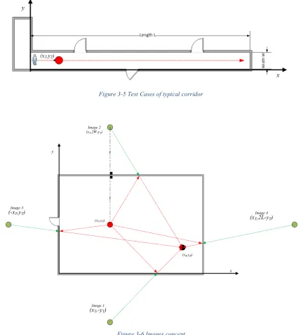
Figure 3-5 Test Cases of typical corridor ... 17!
Figure 3-6 Images concept ... 17!
Figure 3-7 Simulated Frequency Response at different points along a corridor ... 18!
Figure 3-8 theoretical PDP and Frequency response at x=8 ... 19!
Figure 3-9 theoretical PDP and Frequency response at x=18 ... 19!
Figure 3-10 RMS Delay Spread for a Corridor for 3 different cases ... 20!
Figure 3-11 General Linear Channel Model ... 21!
Figure 3-12 Channel Impulse Response of the two antenna case ... 22!
Figure 3-13 frequency Response for different values of α ... 23!
Figure 3-14 Dispersive Fading null chart for 2100MHz band (Zoomed) ... 24!
Figure 3-15 Measured Frequency response for a 2 antenna case. ... 24!
Figure 3-16 three antenna case with different DAS splitting arrangement ... 26!
Figure 3-17 Soft Hand off simulation for 3 Antenna scenario ... 26!
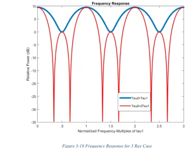
Figure 3-18 Frequency Response for 3 Ray Case ... 27!
Figure 3-19 Simulation and Measurement of Three Antenna Case ... 27!
Figure 3-20 Doppler Shift in a DAS Tunnel deployment ... 28!
Figure 3-21 Dense Indoor Environment (High Rise Hotel). ... 30!
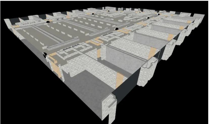
Figure 3-22 3D cross section of IBwave Floor Model for a Hotel ... 31!
Figure 3-23 Geometry of antenna arrangement ... 31!
Figure 3-24 Multiple Contribution Zone ... 32!
Figure 3-25 PDP and Frequency Response for Point 1 ... 35!
Figure 3-26 PDP and Frequency Response for Point 2 ... 35!
Figure 3-28 PDP and Frequency Response for Point 5 ... 36!
Figure 3-29 PDP and Frequency Response for Point 4 ... 36!
Figure 3-30 Service Count Simulation (11-Antenna Design) ... 37!
Figure 3-31 Nature of Path Simulation (11-Antenna Design) ... 37!
Figure 3-32 Soft HandOff (11-Antenna Design) ... 37!
Figure 3-33 Soft-Hand off Area calculations for 2 different designs ... 38!
Figure 3-34 Service Count Area calculations for 2 different designs ... 38!
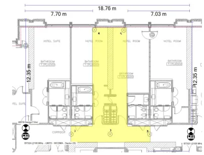
Figure 3-35 Example of an Open office indoor environment ... 39!
Figure 3-36 Simulcast Coverage Area of a stadium sector covered by 4 Antennas ... 40!
Figure 3-37 Simulcast Coverage Area of a stadium sector covered by antennas on the edges ... 40!
Figure 3-38 PDP of Stadium seating test path ... 41!
Figure 3-39 Frequency Response of Stadium seating test path ... 41!
Figure 3-40 RMS delay Spread and Coherence Band Width for Stadium Example ... 42!
Figure 4-1 Open office with 4 antennas ... 45!
Figure 4-2 Soft Handoff Simulation ... 45!
Figure 4-3 PDP of open office along the edge of the room ... 46!
Figure 4-4 Arrival time for direct rays only ... 47!
Figure 4-5 RMS Delay Spread of open office along the edge of the room ... 47!
Figure 4-6 Arrival time for direct rays and reflections ... 48!
Figure 4-7 PDP of open office along the edge of the room (direct ray + reflections) ... 48!
Figure 4-8 Expected PDP for open office example ... 49!
Figure 4-9 CPICH Delay and Delay Spread for Palm Jumairah Tunnel ... 54!
Figure 4-10 Absolute Delay for Active and Passive tunnel DAS ... 54!
Figure 5-1 GNU-Radio Channel Sounder Transmitter. 32MHz BPSK modulated signal 58! Figure 5-2 GNU-Radio Sliding Correlator Channel Sounder Receiver ... 59!
Figure 5-3 Sliding Correlator Output for a two path emulated channel ... 59!
Figure C-2 Soft Hand-Off Simulation (11-Antenna Design) ... 79!
Figure C-3 Service Count Simulation (11-Antenna Design) ... 80!
Figure C-4 Nature of Path Simulation (11-Antenna Design) ... 81!
Figure C-5 Nature of Path Simulation (22-Antenna Design) ... 82!
Figure C-6 Soft Hand-Off Simulation (22-Antenna Design) ... 83!
Figure D-1 Dispersive fading nulls for 2100MHz Ban ... 85!
Figure D-2 Dispersive fading nulls for 1800MHz Band ... 86!
Figure D-3 Dispersive fading nulls for 900MHz Band ... 87!
List of Tables
Table 3-1 Propagation Delay for Common DAS cables ... 10!
Table 3-2 Estimated Wall Penetration Delays for simulation Materials ... 13!
Table 3-3 Wall Materials Simulation Parameters ... 33!
Table 3-4 DAS cable length to Antenna Units ... 33!
Table 3-5 Receive Points Analysis ... 34!
Table 5-1 SDR Sounder Charecteristics ... 59!
Glossary
BER Bit Error Rate
BTS Base Transceiver System CDMA Code Division Multiple Access CIR Channel Impulse Response. CPICH Common Pilot Channel DAS Distributed Antenna System. DDDAS Distributed Delay DAS.
EIRP Effective Isotropic Radiation Power
GSM Global System of Mobile communications. PDP Power Delay Profile.
RBS Radio Base Station
STDCC Swept Time Delayed Cross-Correlation channel sounder TOA Time of Arrival.
Chapter 1
!
Introduction
1.1.# Motivation#
Being in the wireless industry for the last 9 years I have observed a need for a test equipment and design tools that predict and estimate the final performance of a deployed Distributed Antenna System (DAS) site. With Data technologies advancing from GPRS, EDGE, HSPA and LTE, the demand to predict final throughput was deemed critical from there being no way to address this demand without full deployment of the project. My initial hypothesis about such tool was a high resolution channel sounder to collect Path Loss values and indoor multipath information. A considerable amount of time was spent building a Software Defined Radio (SDR) channel sounder to prove the concept. Channel sounder researches and literature were surveyed in a quest for this ultimate indoor design verification tool. I noted that a very important part of the indoor channel was overlooked in these researches, the effect of the DAS design on the channel. The characterization of indoor channel was basically based on simple case of one transmitter. For the Distributed Antenna Systems, as the name suggests, the transmit antenna is actually a modified distributed version of standard antenna. The delays introduced by this distributed nature is much higher than the indoor multipath case for the intended coverage area. Although these delays are a direct result of the DAS design, delays are not considered in the DAS design process.
Based on these findings I decided to direct my effort to the understanding of the delay attributes of DAS systems on indoor wireless channels and possible applications for indoor localization and positioning.
1.2.# Thesis#Overview#
Chapter 2 gives a background of DAS types and definitions, both active and passive DAS.
Chapter 3 evaluates sources of delays in DAS, analysis on the effects of absolute and relative delay for simulcast situations compared to indoor reflections, describes a general DAS model and delay mapping concept. Basic cases of simulcast transmission are analyzed and case studies are presented for important propagation environments
Chapter 4 examines practical delay adjustment techniques and introduces a design concept to optimize location finding. Fingerprinting for indoor positioning is briefly described in this chapter.
Chapter 5 sheds light on the Channel Sounding applications for DAS and introduces a testing procedure for optimizing DAS delays
Chapter 2
!
Overview of DAS systems
2.1.# Introduction#
Passive and active Distributed Antenna Systems (DAS) have been in the mobile industry for the past three decades as a means of delivering quality mobile services and public safety communications for indoor subscribers. The need for DAS has increased over the last decade with the introduction of new cellular standards and the exponentially increasing data demand. Often, the indoor channel characterization concentrates on the case of single transmitting antenna. In this paper, we will study DAS systems with emphasis on their delays specially in simulcasting deployment where multiple antennas transmit the same signal to the indoor environment. The available studies of the DAS introduced delays and their effects on the indoor channel properties are not sufficient. This paper examines also the effect of delays on the fading characteristics of the channel for different delay profiles.
DAS can be classified into two major categories: Passive DAS and Active DAS. A Passive DAS system utilizes a dedicated indoor Base Transceiver Station (BTS) to distribute its signal to multiple indoor antennas using a passive distributing network. The passive network is formed of Coaxial cables, equal and non-equal power splitters. On the other hand an active DAS system distributes the signal through amplification of the signal electronically on the Forward and Reverse path, utilizing optical fiber, network cables, and other types of low-loss physical media to deliver better signal with the target of achieving better quality of service. A combination of active and passive DAS is often referred to as Hybrid DAS.
advanced every day promising better quality signal delivery for traffic hungry user equipment’s (UE).
2.2.# DAS#Types#and#Architecture#
The detailed comparison and classification of DAS equipment is outside the scope of this thesis. However, an overview of the commonly used transport media and topology will help us understand the sources of signal propagation delays.
2.2.1! Passive!DAS!
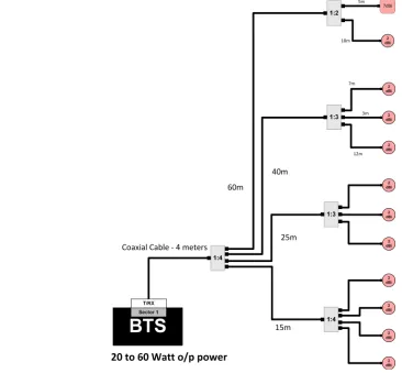
[image:15.612.96.462.340.679.2]Passive DAS refer to the use of coaxial cables, power splitters and antenna to distribute the signal from the BTS, NodeB or eNodeB (hereafter referred to as Signal Source) in an indoor location to the antenna to deliver a signal to the subscribers. Passive, as opposed to Active, does not utilize any kind of electronic signal amplification at any
Figure 2-1 Sample Passive DAS Schematic representation
stage after the original signal source. The available power to distribute is limited to the signal source power Figure 2-1.
A Passive DAS design is characterized by high cable losses, is difficult to balance to provide the same output EIRP from each antenna, has a limited area span from the BTS room depending on the BTS power, and lower SNR on the uplink (reverse) path due to the initial attenuation of signal from mobile to the receiver amplifier.
2.2.2! Active!DAS!
An Active DAS system, on the other hand, solves the problem of limited available power at the signal source that is distributed to many indoor antennas. An active system distributes and amplifies the signal through several amplifiers, each feeding a group of antennas. In uplink, or reverse path, active DAS amplifiers pick up the signal as close as possible to the UE. Having the first amplifier stage closer to the user equipment enhances the Signal-to-Noise ratio (SNR) significantly. The main advantage of Active DAS is the use of a low intermediate frequency on different transportation media, (fiber, twisted pair or thin coaxial) to achieve lower losses than the RF signal on coaxial cables, thus carrying the signal longer distances and across wider coverage areas. The Active DAS then converts the signal back to the original RF Frequency.
and Remote-end units. Some architectures have an additional unit between the front end and the head-end. Specific naming of these units depends on the manufacturer or vendor. Active equipment units are sometimes referred to as Main unit and Remote unit. Transport medium can be optical fiber, twisted pair or thin coaxial cables. With all active equipment sharing the same concept of distributing RF signal from a single point to multiple antenna, the topology depends mainly on the transport medium. For example, a product using twisted pair cables to transmit the signal and DC power to a remote amplifier has a low amplifier power, typically less than 1 watt. This type of amplifier in typical indoor deployment requires using several remote units in the same floor to achieve the required coverage levels. With power amplifiers below 1 watt feeding antennas, several amplifiers will transmit the same signal on the same floor with overlapping coverage areas. These overlapping coverage areas will receive a signal from different antennas with different arrival times. Such overlapping coverage areas can exceed 30% of a given floor layout.
2.2.2.1
!
Digital and Analog Active DAS
A Digital DAS system digitizes the signal source at very high speed through Analog to Digital Converters (ADCs) before transporting it to the remote-end. At the remote-End equipment, the signal is converted back to its original analog form using Digital to Analog converters (DACs) and then amplified to the rated amplifier power.
The use of data converters and digital transport technology minimizes the effect of loss and noise in transport medium thus achieving better signal quality in both the forward and reverse path. Additionally, the digital DAS system can digitally control the delay to each individual remote-end amplifier for multiple remote deployments.
2.2.3! Hybrid!DAS!
It is a common practice in DAS industry to identify an Hybrid DAS as an Active system utilizing high power amplifiers since Hybrid DAS has enough power to drive a large network of passive splitters and coaxial cables similar to the Passive DAS. While this definition is common, we observe that a hybrid system is better defined as the system where a passive distributing network is employed to deliver power RF power to one or more antennas in parallel to an active DAS of any Power rating. The Characteristics of delays of a Hybrid System defined in this way exhibits a specific pattern dissimilar to the common definition.
2.2.4! DAS!RF!Power!
Typical values of head-end RF power range from 0.5 watt to 40 watts. For Middle East indoor DAS designs, an average EIRP varies between 5 to 10 dBm per channel due to the heavy use of concrete Middle Eastern building structures. For such environment, a low and medium power DAS equipment is connected to maximum of 1 to 5 antennas while a higher power remote-end can support up to 20 antennas depending on the design of the passive RF distribution network.
2.3.# Simulcasting#Concept#
Simulcast in DAS refers to utilization of two or more head-end units to transmit the same signal from the same signal source. This concept is used to extend the coverage map of the cellular sector in areas where more coverage is required without adding more capacity to the system.
Chapter 3
!
DAS Delays
3.1.# Sources#of#Delays#in#DAS#Systems#
To analyze the effect of DAS delays on the wireless channel, we first identify two different ways to measure the delay: Absolute delay and relative delay. The absolute delay is the time needed for the signal to travel through all the system components from the signal source to the UE taking the DAS RBS RF port as the reference of measurement. The relative delay on the other hand is the time of arrival relative to the first version of the signal.
3.1.1! Cable!and!filter!Delays!
Electromagnetic waves propagate in different mediums with different velocities. The velocity of Electromagnetic waves in fiber, copper and coaxial cables (non-magnetic mediums) depends on the dielectric constant ! or refractive index " of the cable. For Coaxial cables, propagation velocity is given by [17]
#$% = '
! (3.1)
where c is the speed of light in vacuum. Cable manufacturers quote the Velocity Factor #( for cables relative to ' instead and is defined as the percentage of the velocity of electromagnetic signals in the cable to the velocity of light in vacuum. Hence VF in Coax is given by
#(% = 100
! (3.2)
For Optical fiber cables, the refractive index " is, by definition, the ratio of the speed of light in vacuum to the speed of light in the optical cable. Hence Velocity factor in fiber is given by
#( = 100
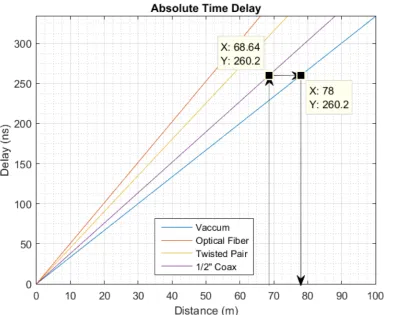
Figure 3-1 presents the propagation delay values for common cables used for DAS. A typical value of 5ns/m for fiber and 3.8ns/m for common Coaxial cable (LDF4-50A) are used. To put this delay value in perspective, the chip duration for WCDMA is 260.4ns; hence a generic ½” coaxial cable of 68m introduces a propagation delay equivalent to one chip in WCDMA as exhibited in Figure 3-1
Cable Property
Type of Cable Braided Coax
(RG-58A/U)
Foam Coax
LDF4-50A Optical Fiber
Twisted Pair CAT5E
Velocity Factora(%) 66 88 67 74
velocity (m/s) 197863022 263817363 200860946 221846418
Propagati on Delay (ns/m) 5.054 3.791 4.979 4.508
a.Reference to speed of light in vacuum of 299,792,458 m/s
[image:21.612.109.517.357.672.2]Table 3-1 Propagation Delay for Common DAS cables
3.1.2! Hardware!Delays!
Delays due to the electronic circuitry of active DAS are here referred to as Hardware delay. These delays are always constant for an individual active DAS product. It is very rare that two types of active products are used in the same indoor site to cover the same location, although it can be used in the instance of upgraded sites. Assuming single product usage, HW delays are consistent for all devices and add to the absolute delay. However, relative delays are only triggered by differences in cable lengths. Quoted value for the hardware delays for an Analog DAS product is less than 500ns and 12µs for the Digital DAS product [29] [31].
3.1.3! Generalized!DAS!model!
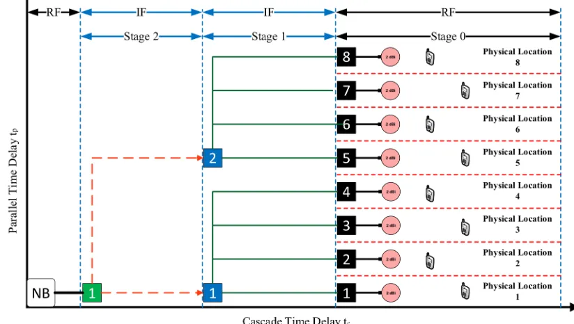
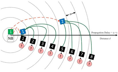
[image:22.612.97.509.453.686.2]requirements. A purely passive DAS will only have Stage-0. An Active DAS of a single star connection topology will have both Stages-0 and Stage-1. A double star topology will have Stage-0, Stage-1 and Stage-2 and so on for Cascaded DAS systems. Figure 3-2 depicts the general DAS model mapped on a Delay Map where no two equipment have the same absolute delay. Each box indicates an active equipment device. The boxes are marked with numbers labeling the corresponding device. The two axes have time dimensions and the absolute delay is the sum of the cascade delay component τc and parallel delay component τp .where cascaded and parallel subscripts refer to hypothetical direction of delay measurement.
3.1.4! Delay!Mapping!Concept!
[image:23.612.96.508.71.325.2]It is the industry standard to have Power budget and Antenna EIRP reports as the main design deliverables along with the indoor floor layouts. Recently, DAS software tools introduced specific reports to help deployment teams in their work by providing details on antenna orientation, cable routing and cross references. A very important yet missing concept in these deliverables is the calculation of delays from source to antennas and a mapping to their physical locations. The simplest form of such map can be a table with calculations and physical installation location. A more detailed representation can be as
presented in Figure 3-2 and Figure 3-3. The importance of a delay map will be clear in the discussions of indoor positioning information available from DAS. A single glance to a delay map should be sufficient to identify the possible locations and causes of ambiguity in indoor Time of Arrival (TOA) ranging. Such delay map should be added to the site database, planned at design and verified at commissioning stage.
3.1.5! Wall!Penetration!Delay!
Penetration of walls on the path of the signal will introduce a delay equivalent to the time of propagation in material of a certain relative permittivity. The maximum penetration path is determined by Snail’s law to avoid total internal reflection inside the wall. Table 3-2 shows the maximum delay for the wall material for a given thickness. Maximum penetration path accounts for the real path at the critical angle inside the wall.
Stone Brick Concrete Wood Glass Fiberglass Rel. Permittivity 4 6 1.8 6.7 5.2 Material Thickness (m) 0.15 0.2 0.1 0.01 0.01 Velocity factor 50.00 40.82 74.54 38.63 43.85 Propagation Delay
(s/m) 6.67E-09 8.17E-09 4.48E-09 8.63E-09 7.61E-09 Critical angle (rad) 0.2527 0.1674 0.5890 0.1498 0.1935 Maximum Penetration
Path (m) 0.1549 0.2028 0.1203 0.0101 0.0102 Maximum Penetration
delay (ns) 1.034 1.657 0.538 0.087 0.078
3.2.# Effect#of#absolute#delay#introduced#by#DAS#
The absolute delay of Active DAS system will be seen by the source as an offset to cell radius. The distance at which the UE is located away from the source is increased by an offset equivalent to the same delay in a vacuum. Figure 3-1 can be used to estimate the effective location of the UE as seen by the source. Depending on the specific technology, the signal source with feedback from the UE estimates the distance based on the propagation delay by assuming propagation in a vacuum (or any predefined propagation model). Methods like Time of Arrival (TOA) and round trip time (RTT) are used for ranging. A hybrid DAS signal source will see the subscribers’ UEs as two groups. The first group is very close to the source communicating through passive DAS and a second distant group communicating through the active DAS with an offset in distance equivalent to the hardware and fiber delays. Figure 3-4 illustrates this effect where d0 corresponds to
maximum delay in passive DAS. d1 equivalent to minimum active hardware and cable
delays, d2 is the distance of the farthest UE. It is important to carefully study and consider
[image:25.612.97.514.396.679.2]relative delays for indoor sites with a mix of passive and active DAS to avoid possible
channel degradation and interference due to the relatively high hardware delays in overlapping coverage area.
3.2.1! Accumulated!Propagation!Delay!
The accumulated propagation delay for a given antenna n is the summation of all delays accumulated over the signal path to this antenna according to the DAS model in Figure 3-2 and is given by
+, = -. + (1. ∙ 34.) 6
.78
(3.4)
where n is the antenna number, i is stage number and I is the total number of stages, ki is the active equipment hardware delay, li is the cable segment length and Pdi is its
propagation delay per unit length of the cable.
3.2.2! Manipulating!DAS!delay!!
3.3.# Effect# of# relative# delays# introduced# by# DAS# on# Channel#
Impulse#Response#
For the selected case studies and antenna deployments, the effect of indoor multipath can cause a negligible delay in the range of several nano seconds as in corridors to larger delays but with high reflection and propagation losses that minimize their effect on the channel characteristics. Thus it’s safe to exclude these components from the study of power delay profile caused by the DAS. On the other hand, the relative delays caused by DAS can range from 80~300 with comparable power levels at significant percentage of indoor coverage area. To further justify this assumption, simulations of the first level of reflections using one transmitting antenna was conducted in the corridor and Open-Office room of Figure 3-5. Wall and ground reflection losses are assumed to be 6.5dB. The transmitting and receiving antennas are placed at coordinates (xT,yT,hT) and (xR,yR,hR).
Comparing the result of single antenna with reflections taken into account against another two cases where two antennas are placed symmetrically across the corridor at x=3 and x=37m. A relative delay of transmission from the antenna equivalent to a cable of 40m length is assumed. We can safely conclude that we can neglect the reflection components in channel merits related to delays in the presence of a DAS simulcast system. Figure 3-10 shows the RMS delay spread for the three different cases of the corridor example.
!
3.3.1! General!formula!for!Simulcast!DAS!Channel!delays!
The simulcast channel model caused by DAS is identical to a multipath channel where delay between DAS antennas is the main cause of the multipath nature. Indoor locations receiving signals from more than one antenna can suffer from dispersive fading. This fading envelope can change the channel classification from wideband to narrow band, in addition to the introduction of inter-symbol interference caused by path delays.
The general formula governing multipath linear channel h(t) is given by corresponding to Figure 3-11 [7].
ℎ : = ;<=(: − +<) ?@A
<78
(3.5)
B C = ;<D@EFGHIJ
?@A
<78
(3.6)
K : = % ;<L : − +< + M(:) ?@A
<78
(3.7)
where
s(t) is the input signal,
H(f) and h(t) are the channel spectrum and impulse response, respectively
v(t) is a zero-mean white Gaussian noise random variable with power spectral density of No/2, and
τ
m is the mth component delay.We are interested in the study of the channel in simulcast scenarios discussed in the following section.
3.3.2! Simulcast!deployment!scenarios!
3.3.2.1
!
Scenario I: Direct indoor with two antenna in an open area
A common deployment scenario in an indoor environment is where UEs are stationed in an open area and receive signals from two DAS antennas.. Such a case can apply to theaters, food courts and stadium seating where UEs are almost stationary. Corridors are another common situation with slowly moving UEs. The resultant channel is described byFig.3 with frequency response equal to
B(C) = %1 + ;D@EFGHI (3.8)
Where +%is the relative delay between the two received signals and αis the relative amplitude of the delayed signal from the second antenna. For the worst case, this factor is
assumed to be 1. Lower values of α will have a scaling factor equal to ANO
A@O on the peak-to-peak amplitude of the sinusoidal channel frequency response pattern as in Figure 3-13. The resultant channel is a frequency selective fading channel with nulls at
C =(2" + 1)
2+ (3.9)
where n is an integer≥ 0.
A set of charts are produced to locate these nulls corresponding to certain cable length or delay τ (Appendix D ). Figure 3-14 show an examples for 2110MHz band chart. Values of delay τare limited to a certain range of interest for better appearance. The colored lines represent the location of nulls for different values of n. a vertical line intersects the colored lines at null locations. Sliding this line to the right or left gradually changes the null locations and separation corresponding to a moving receiver around the initial point.
Figure 3-14 Dispersive Fading null chart for 2100MHz band (Zoomed)
3.3.2.2
!
Scenario II: Three Antenna in an Open Area
Another simulcast situation of interest is where the UE is in the coverage of three antennas. Typical examples of these environments include theaters and stadium seating. Mobile users are almost static in this case. So far, a widely accepted approach to cover high capacity stadium is to divide seating area into sectors of few thousand subscribers. To achieve high isolation between these sectors antennas are positioned on the edges of the sector radiating inwards (two on the sides and one at the back) to increase received signal levels and increase isolation relative to adjacent sectors. Effects of delays are not accounted for when designing for such situation. Similar to the two antenna case, the frequency response of this channel of three antennas is given by
B C = %1 + ;AD@EFGHIQ+ ;FD@EFGHIR (3.10) ;A and ;F equal 1 for the worst case where the 3 signals from the 3 different antennas are exactly equal in power. There are unlimited possibilities for the frequency responses for different combinations of ;A%, +A%, ;F and +F that can be accurately predicted by ray tracing simulations to obtain the frequency responses. Figure 3-17 exhibits that more than 60% of the area has a relative received power within 6dB which translates to α = 0.5 . For areas where one of the received signals rays is very weak (α is very small) presents the effects of a 2 antenna scenario. We can simplify the problem by considering a common deployment cases where +F = +A and +F= 2%+A as shown in Figure 3-16.
The channel impulse responses for these cases are given by
B C = %1 + 2D@EFGHIQ (3.11)
B C = %1 + D@EFGHIQ+ D@ETGHIQ (3.12)
Figure 3-19 displays the frequency response for a given +A for both cases. The frequency axis is normalized to +A. It is clear that an indoor RF designer should avoid the second splitting arrangement where the three antennas are connected with constantly progressive delays.
Figure 3-16 three antenna case with different DAS splitting arrangement
3.3.2.3
!
Scenario III: Tunnels and Outdoor DAS
Outdoor DAS (sometimes referred to as Street DAS) refers to the deployment of Active DAS in outdoor environment for coverage extension or capacity enhancement. Outdoor DAS deployment is usually characterized by High Power Amplifiers, low numbers of antenna per remote equipment and longer distance span from head-end to remote-end equipment over optical fiber cables. Tunnels can have remotes placed at distances approximately 1km apart with hundreds of meters of radiating cables (cable antenna) to distribute the signal in the tunnel. Outdoor and street DAS are intended to cover large outdoor areas like college campuses, outdoor malls and outdoor exhibition venues. For overlapping coverage areas, relative delays will be contributed mainly by fiber optic delays in the order of few micro seconds. Such large delays should be eliminated and brought down to a value that the technology is capable of handling for simulcast cases and Handover between different sectors. Cable spooling or digital delay is used to balance delays. A State of the art digital DAS has a 1µs delay adjustment resolution over the fiber. Moreover, the known effect of Doppler Shift caused by the relative motion of the transmitter and the receiver has a different effect in tunnels with DAS simulcast deployment. The receiver will be relatively moving away from a transmitter but at the same time approaching another transmitter. This will result in having a positive and negative frequency shifts at the same with one of these shifts is also delayed in time. Figure 3-20 represents a DAS in a tunnel showing the resultant signal smeared frequency.
!
3.3.3! Relative!Delay!Effects!for!Different!Cellular!Technologies!!
In addition to the dispersive fading effect on the channel, relative DAS delay in an indoor site causes delay spread and inter-symbol interference. This effect is most significant for WCDMA technology where the symbol rate (chip rate= 3.84MHz) is the highest in all existing cellular standards. The highest rate for EDGE is 325KHz while LTE has hundreds of subcarriers with a symbol rate of 15 KHz. Direct sequence spread spectrum systems like WCDMA have to rely on rake receivers and frequency domain equalization to untangle ISI [16] .In WCDMA, relative delays below one chip duration of 260.4ns will cause delay spread and inter-chip interference. The typical distance of 30m or less between indoor antennas causes a delay equal to half the chip duration which affects signal quality. RAKE receivers are able to resolve the second path only if the delay exceeds one chip period, or equivalently, antennas are separated over 68m apart. Unfortunately, this will impose harder constraints on the designer and might not be possible for all RF designs. A solution is avoiding two serving antennas in the same open area unless there is sufficient delay between them. Also assuring there is ample RF isolation for antennas in close vicinity of each other. i.e., avoid overlapping coverage areas of comparable power.
It is noteworthy to highlight that current RF prediction models and design tools do not take into account the effect of simulcasting or DAS delays. Software tools that use Ray Tracing prediction models can be improved by calculating delays to predict the exact channel impulse response for a given indoor location and, consequently, help predict BER performance and expected data throughput for any technology.
3.4.# Case#Studies#
In this section we will study a specific cases and apply the analysis of DAS delays and their effect on the indoor channel.
3.4.1! Dense!Indoor!Environment!with!Corridors!
of RF power and active equipment needed to generate enough power to penetrate the dense structure at the entrance of the hotel rooms (Toilets, Wooden closets, air ducts, etc.). Figure 3-21 presents a floor layout of the clock tower hotel in Makkah, KSA (the 3rd tallest building worldwide).
Delivering the required coverage levels at room edges is nearly impossible when coverage from nearby outdoor cellular sites is significantly high. Adding more indoor antenna to get the required coverage levels also adds more sources in a simulcasting configuration and changes the channel characteristics in the overlapping coverage areas. IBwave software is used to simulate the overlapped coverage area with its proprietary fast ray tracing algorithm. A very detailed 3D model of the building was developed using material types in AutoCAD files and matching IBwave material definition (Figure 3-22). Wall material parameters was calibrated using feedback from several CW tests and site surveys. The resultant 3D model includes effects of not only brick and concrete walls but also the false ceilings, large metal pipes in Electromechanical Risers, toilet wall partitions and wooden cabinets. All simulation were run with a resolution of 15cm at hR=1.5m above
[image:41.612.94.510.81.322.2]ground applying a fast ray tracing algorithm. Table 3-3 shows the material parameters used in simulations antenna height hT=2.5m.
Cable lengths and distances measured on IBwave layout are in the x and y directions. To account for the direct path in the z dimension we use equation (3.13) corresponding to Figure 3-23 where l is the direct ray distance from Antenna to receiver and d is the horizontally measured value from IBwave. In our case, the difference between measured and actual path is very small for d >5m that it can be neglected.
1 = % 4
cos tan@Aℎ[− ℎ\ 4
(3.13)
[image:42.612.100.516.75.321.2]To obtain an indication of coverage overlap, we examined three different prediction types for two proposed designs with 11 and 22 antennas respectively. Nature of path, service count and Soft handoff simulations were compared. The Soft hand off simulation is used to predict the relative coverage levels from each antenna. To accomplish this, we temporarily assign a different sector to each antenna for the purpose of simulation only. However, in Simulcast configuration, all antennas are connected to the same RF BTS sector thereby transmitting the same signal. The Soft Handover simulation calculates the relative signal levels at each point in the layout and calculates the percentage of area with certain limits. For this study we will concentrate on 8~10dB difference between the signals from different antennas. Figure 3-32 , Figure 3-30 and Figure 3-31 show soft handoff, service count and nature of path simulations respectively. Nature of path simulation indicates the type of dominant signal path which are either a Diffracted Ray, Direct Line of Sight (DLOS), Direct Non Line of sight (DNLOS) or multiple contributors. Since our main concern is in areas with relatively similar received power from more than one antenna, we
are concerned only with the multiple contribution zone in the nature of path simulation Figure 3-31.
A detailed analysis on the five points shown in Figure 3-24 is conducted. Wall penetration delays is assumed to be an exaggerated value of 5ns for all wall types. The increase from the values calculated in Table 3-2 accounts for wall thickness variations among different floors of the HI-Rise buildings. Concrete walls and columns are thicker in
the lower floors compared to the top floors of the building. Table
3-5
shows the extracted values from different simulations from IBwave. For each of the five points, we have the received signal strength (Rx power), path length and the corresponding propagation delay. Moreover, we calculate the wall penetration delay based on a 5ns assumed wall penetration delay multiplied by the number of walls in the signal path from source to receiving point. For the given design, cable lengths of Active DAS are listed in Table 3-4 Assuming a cable with VF=84Type Stone Brick Concrete Wood Glass Fiberglass Metal sheet
Diffraction loss (dB) 20 19 22 17 20 20
Incident loss (dB) Max 36 35 33 34 36 36
Min 12 12 9 13 12 12
Reflection loss (dB) 9.52 7.51 16.2 7.08 8.17 0.05
Rel. Permittivity 4 6 1.8 6.7 5.2 1
Rel. Permeability 1 1 1 1 1 20
Conductivity (S/m)
2000MHz 0.04 0.08 0.03 0 0.03 11111.11
2400MHz 0.05 0.09 0.04 0 0.03 13333.33
interpolated for
2170MHz 0.044 0.084 0.034 0 0.03 12055.5535
Transmission Loss (dB)
2000MHz 4.48 12.08 4.24 1.9 1.62 951.94
2400MHz 7.57 14.16 5.05 1.9 1.66 1014.73
interpolated for
2170MHz 5.79325 12.964 4.58425 1.9 1.637 978.62575
Material Thickness
[image:44.612.101.522.344.582.2](m) 0.15 0.2 0.1 0.01 0.01 0.01
Table 3-3 Wall Materials Simulation Parameters
Using the information about signal power and path delay we ran a series of MATLAB simulations to estimate the channel characteristics both in time domain and frequency domain. Simulation in time produces the Power Delay Profiles while the frequency simulation produces the channel frequency response for a given location.
! Point!1! ! ! Corridor! ! !
Source!ID! Rx!Power!(dBm)! Path!length!(m)! Pd!(ns)! Penetrations! Type! Wall!Delays!
2! B75.20! 19.63! 65.5! 1! DNLOS! 5.00!
3! B58.57! 9.32! 31.1! 0! DLOS! 0.00!
5! B70.61! 36.73! 122.5! 0! DLOS! 0.00!
9! B67.83! 27.28! 91.0! 0! DLOS! 0.00!
11! B57.80! 9.30! 31.0! 0! DLOS! 0.00!
! ! ! ! ! ! !
! Point!2! ! ! Corridor! ! !
Source!ID! Rx!Power! Path!length!(m)! Pd!(ns)! Penetrations! Type! Wall!Delays!
3! B53.52! 5.31! 17.7! 0! DLOS! 0.00!
4! B81.61! 24.86! 82.9! 0! Diffracted! 0.00!
5! B71.55! 41.91! 139.8! 0! DLOS! 0.00!
9! B69.25! 31.94! 106.5! 0! DLOS! 0.00!
10! B75.87! 24.50! 81.7! 0! Diffracted! 0.00!
11! B61.40! 13.76! 45.9! 0! DLOS! 0.00!
! ! ! ! ! ! !
! Point!3! ! ! Corridor! ! !
Source!ID! Rx!Power! Path!length!(m)! Pd!(ns)! Penetrations! type! Wall!Delays!
3! B62.06! 14.25! 47.5! 0! DLOS! 0.00!
5! B69.44! 32.14! 107.2! 0! DLOS! 0.00!
9! B66.14! 22.62! 75.5! 0! DLOS! 0.00!
11! B52.31! 4.71! 15.7! 0! DLOS! 0.00!
! ! ! ! ! ! !
! Point!4! ! ! Guest!Room! ! !
Source!ID! Rx!Power! Path!length!(m)! Pd!(ns)! Penetrations! Type! Wall!Delays!
2! B84.69! 30.94! 103.192! 2! DNLOS! 10.00!
3! B84.2! 13.87! 46.252! 4! DNLOS! 20.00!
11! B97.71! 15.93! 53.141! 5! DNLOS! 25.00!
! ! ! ! ! ! !
! Point!5! ! ! Guest!Room! ! !
Source!ID! Rx!Power! Path!length!(m)! Pd!(ns)! Penetrations! Type! Wall!Delays!
2! B84! 30.94! 103.192! 2! DNLOS! 10.00!
3! B98.9! 15.79! 52.675! 6! DNLOS! 30.00!
[image:45.612.98.519.62.531.2]11! B86! 13.87! 46.252! 5! DNLOS! 25.00!
3.4.1.1
!
Channel Power Delay Profile and Frequency Response
Figure 3-26 to Figure 3-29 show the Expected Power Delay profile of the channel as a result of the reception of the signals in Table 3-5 adjusted by delays of Active DAS Stage-1 cables in Figure 3-2.
Figure 3-25 PDP and Frequency Response for Point 1
Notes on Multipath Rays: to the best of our knowledge the Ray tracing method implemented in IBwave reports the collective power received at a certain point on the layout without information about the relative delay of these paths. However, the relatively small arrival delay of the first level reflections and the reflection loss make it safe to neglect their effect. For instance, the reflection loss of a ground bounce in the corridor is around 7.5dB delayed by 2.4ns from the direct path at 10m distance from the antenna. The 2.4ns is significantly small compared to the delays caused by DAS. From the PDP and channel response figures, we can conclude that the highest two arrivals have the most significant effect on the frequency response. The third highest component will have a ripple effect on the response according to its relative arrival time and power, which is very clear for point 5 as exhibited in Figure 3-28. The significant factor determining the channel response for an indoor DAS deployment is the DAS delay and power received from simulcasting DAS antenna.
Figure 3-32 Soft HandOff (11-Antenna Design)
3.4.1.2
!
Effect of Antenna Count
Figure 3-33 and Figure 3-34 display a comparison between two designs comparing the covered area percentage served by a specific number of antenna with signal levels above -90dBm (Figure 3-34), And the percentage of area with certain relative received power (Figure 3-33). It is clear that adding more antennas will reduce the area of single antenna dominance and increase the area of overlap converting them to multiple contribution zones with more dispersive fading effect.
[image:49.612.89.528.381.681.2]Figure 3-33 Soft-Hand off Area calculations for 2 different designs
3.4.2! Open!office!environment!
Figure 3-35 shows an Open-office environment with the expected coverage contours of each antenna. Open-Office environment is characterized by low losses and average capacity requirements. Although such environment is considered a simple design problem for an RF engineer, delay effects are most prevalent in this environments. Detailed analysis of delays in an open-office example will be discussed in Chapter 4.
3.4.3! Theater!and!Stadium!Seating!
[image:50.612.141.473.76.390.2]Theaters and Stadiums are high capacity venues with mostly line of sight coverage.
requirements in cases where dominance is required over high level nearby Macro-Cellular coverage. Obtaining an RF isolation between RF sectors in this open environment is a challenge. RF isolation is typically achieved by using special stadium antenna with high directivity and narrow beam width mounted at a high altitude structures. Or by multiple antenna per sector surrounding the intended coverage area at the seating level. Isolation in the latter case requires placement of directional antenna at the sector borders resulting in a simulcast coverage area in the middle. Figure 3-36 shows an example of the first case with
[image:51.612.97.473.473.692.2]4 antenna mounted on the roof structure (not shown in figure) and Figure 3-37 shows the case of antenna on the edges at the same level of the spectators with more than 70% of the area in simulcast coverage. Simulations for frequency responses and PDP for a test path in the middle of seating from top to bottom is shown in Figure 3-38 and Figure 3-39
Simulations for the RMS delay spread and Coherence bandwidth (calculated here as 20% of the reciprocal of the RMS delay spread) is shown in Figure 3-40. Several simulation results of different combinations of antenna transmit delays were examined. Simulation for the PDP and CIR for the complete seating area was done for a given transmit delay and dimensions with extreme data output size and processing requirements. Some
[image:52.612.90.521.86.288.2]combinations of transmit delays produced better frequency responses for the examined frequency ranges at specific locations. Best RMS delay spread results were achieved by balancing the transmit delay.
[image:53.612.92.472.333.592.2]It is clear that combining delay measurement results with the ray tracing computations produces detailed channel information and can lead to accurate performance estimation for high capacity DAS sites. It is the author’s belief that a more advanced algorithm can be devised to optimize delays to reduce dispersive fading for important venues like stadiums. For instance, since the frequency response is a sum of sinusoids, the transmit delays of the 3-antenna case can be adjusted to produce a frequency response with a relatively large period of null repetition in frequency domain avoiding low coherence bandwidth in areas of interest.
Chapter 4
!
Engineering DAS delays for Indoor Positioning
Application
The U.S. Federal Communication Commission (FCC) Phase-2 E911 emergency positioning requirements mandate that cellular network operators are responsible for positioning wireless terminals with an accuracy of 50m and 150m in 67% and 95% of all positioning attempts respectively for UE-based positioning methods. These values are relaxed to 100m and 300m for 67% and 95% of the attempts respectively for network based methods [2].
of DAS can be engineered to provide information about UE location within a given accuracy based on TOA.
4.1.# Distributed#Delay#DAS#concept#
In order to avail the optimum location information from DAS and reduce ambiguity, we must insure that all DAS transmitters have a different distinctive propagation delay. We introduce a new Distributed Delay DAS design concept, A Distributed Delay DAS is a distributed antenna system designed to produce uniform and gradual propagation delay to each antenna in a specific deployment, thus assuring a distinctive delay mapping to different physical antenna locations. The basic concept is to utilize the maximum delay range available from the active equipment and distribute it between consecutive RF amplifier devices. For example, a certain head-end device provides the ability to change digital delays to remote-end equipment from 10µs to 24µs and has a maximum of 8 remote-end devices connected. The delays to these types of remotes must be set to 10µs, 12 µs, 14µs and so on up to 24µs for the 8th remote.
For an analog active system where delays are defined by cable lengths, we achieve
the same result by utilizing the maximum allowable cable length 1. of a given active equipment stage. We define this delay step or separation as
∆+_ %. = (1.−1.)%34.
(`. − 1) (4.1)
where
1. is maximum cable length specific to the active equipment in use in stage-i, 1. is the shortest possible cable length in that specific deployment
`. is the number of parallel cable branches connected to the i-1 stage (number of connected equipment of the i-1 stage)
Note that the only parameter we can control is the amount of equipment in a given stage. While we can utilize all the full capability of the active equipment, we may want to reduce mi in order to increase time separation between transmitters ∆+_ %. . For the system in Figure 3-2 and Figure 3-3, m1=4 and m2=2.
symmetrical coverage levels across the square open-office hall (L=W=40m). Each antenna
is assumed to cover a circular area of radius 4 = aF with a particular coverage threshold.
Antenna-1 is utilized as the time reference. Consecutive antennas will have a ∆+_ %. =
260ns transmission delay over the previous antenna. i.e., signal delays are 0, 260ns , 520ns and 780ns for the 4 antennas respectively. The expected PDP profile in coverage dominance area (green area in Figure 4-2) should have 4 peaks separated 260ns with the highest peak corresponding to the dominant antenna at its assigned delay. These peaks are further shifted in time depending on the relative propagation delay of the signal over the air from other antennas. The fundamental concepts for building a DDDAS is to first have the ∆+_ %A large enough to eliminate ambiguities of TOA estimation caused by multipath
and wall penetration bias. Second, the resultant PDP should be measurable by the deployed technology standard. WCDMA, LTE, CDMA, etc.
Figure 4-3 shows the PDP of 20 points on the test path at the edge of the room (y=40). This path is selected as it represents the points of minimum separation of arrivals for the given antenna and delay arrangement and only direct path is considered.
Figure 4-4 shows the relative arrival time with minimum separation at x=30 around 200ns. Running the simulation for all locations, we can estimate time of arrival window
of 200ns or better can distinguish the location of the peak within the predetermined TOA window which correspond to a specific antenna and hence provide the location information as designed. For receiving points with equal level of power from two or more antenna (e.g., center point of the office) the PDP will have 4 equal peaks received at exactly 260ns apart. Detection of such locations will depend mainly on the complexity of the TOA measurement system. A system that can provide information about first arrival in addition to an indicative measure of successive arrivals will be able to detect the location accurately. An example of such measure is the RMS delay spread or a more complex system that can actually measure the channel PDP. These values of PDP and RMS delay spread can be simulated using ray tracing and verified at deployment stage to form a lookup table of TOA+RMS delay spread values against receiver location. This database can serve as delay-location map for indoor location finding. Figure shows the RMS Delay Spread for the given example. Given the above mentioned assumptions and results we can conclude that a 20m by 20m area resolution or better can be achieved in an open space. This resolution is mainly defined by antenna coverage area provided that time measurement and separation criteria are met. The coverage resolution is improved with dense propagation environments as a
direct result of more antenna and wall isolation. For hotel environment shown in section 3.4.1 each antenna is effectively covering 2 rooms with total area of approximately 200m2
[image:58.612.156.453.405.648.2][image:59.612.217.400.217.437.2]
Figure 4-6 and Figure 4-7 show the previously simulated case with reflections from walls and ground bounce. All wall losses assumed to be 6dB. Although the minimum separation is reduced, only Reflections with significant power levels should be considered in the estimations of required time measurement resolution.
Figure 4-6 Arrival time for direct rays and reflections
[image:59.612.182.406.481.694.2]4.2.# Criteria#for#Distinctive#Mapping#and#Accurate#Ranging#
Consider the PDP in Figure 4-8 corresponding to the antenna arrangement of the previous open office example in Figure 4-1. The time access represents the absolute delay or TOA from the BTS. Relative transmission delay between consecutive antennas denoted
Δτ01,Δτ12 and Δτ23. The shown peaks are grouped in clusters corresponding to a direct ray
and its multipath reflections. The indicated power levels are the maximum expected received power levels from a particular antenna. The actual power levels are scaled according to the location of the receiver. e.g., if a receiver is in the dominant region of antenna-1, only direct ray from antenna-1 and its reflections are present with significant power. A receiver positioned midway between antenna-1 and antenna-4 will receive relatively equal powers from both antenna and hence will have a PDP with the first and last cluster of peaks and the middle clusters will be significantly low. The PDP in Figure 4-7 shows the case where the received power from antenna-1 and antenna-2 are very small compared to antenna-3 and antenna-4. The expected arrival window of the direct ray is shown as a shaded area. The green dotted line indicates the arrival time at a distance D/2 away from the antenna where D=W/2 is the distance between the two antennas.
[image:60.612.105.514.440.658.2]To avoid ambiguity in ranging, it is required to avoid the overlap of arrivals of consecutive clusters. The selection of the minimum required time offset Δτ should take into account a guard period for multipath and wall delays due to penetrations in the given environment. The measurement system should be able to distinguish between the last significant multipath component and the arrival of the following direct ray. We can define the minimum delay separation required for stage-1 as
∆+_ %A ≥ ∆+_%<., = %d + ɛ + :fgh+ i. 34k.f (4.2) where tres is the propagation delay measurement resolution of the system, γ is a factor
accounting for the indoor multipath at stage-0, ε is a wall bias factor and Pdair is the
propagation delay per unit length of free space. The value of ε can be estimated by counting the number of penetrated walls multiplied by the wall penetration time. ε is a characteristic of the propagation environment and can vary from one site to another.
To estimate γ, we assume it corresponds to a ray propagating in free space reflected with no loss off a wall and received with a relative power level above a certain percentage of the direct ray power at the edge of the intended antenna coverage area (center point of Figure 4-1). For a given relative power ratio the assumed reflected ray must have traveled a distance r. The governing relation is
KD1l:mMD%$noDK = 4 K
F
(4.3)
where d is the direct path length. For threshold of 0.1, K = 10%4 and we can write
d = 10%4 ∙ 34k.f (4.4)
for our example 4 ≅ 2%a T
To avoid any overlap caused by higher stages, minimum delay separation of the upper stages must be greater than all relative delays in the lower stage. That is
∆+_ %.NA ≥ (1.%∙%34.) + ∆+_ %. (4.5) The better the resolution of measuring propagation delay, the higher the flexibility in designing and planning Distributed Delay DAS. Equating (4.1) with (4.2) we see that mi
parallel active equipment in a given stage below the design architecture of the active product and will possibly require additional equipment in the higher stages to achieve the required separation in the delay.
4.3.# Measurement# Resolution# Values# for# Different# Cellular#
Technologies#
There are many techniques implemented to measure signal propagation delay of the signal to the UE. Standards define both mandatory and optional parameters such as Time Advance (TA) for GSM, Round Trip Time (RTT) for WCDMA and Propagation Delay (PD) for LTE, to name a few. The detailed study of measurement techniques and accuracy is beyond our scope. However, we will indicate typical values of current standards.
For CDMA system, the “CDMAServingOneWayDelay2” parameter is reported in multiples of 100ns. Further the standard defines optional resolution of 50ns [11]. For WCDMA, the RTT measurement resolution is one chip [12] and the propagation delay can be calculated by subtracting the time needed for the UE to respond (RxTx) type-1, then dividing by 2 [12][13].
For LTE, time advance parameter (TADV) should be reported with a resolution of 2
time slots
Ts
which corresponds to approximately 65ns [14]. The resolution of TA in GSMis too low to suit our application. Although these values are the standard parameters, it is believed that radio base station vendors can provide more accurate non-standardized measurements determining the propagation delay and algorithms to reduce the measurement errors due to multipath in the RF stage.
Realistic values of γ and ε require testing on a real site and with access to RBS measurement capabilities and algorithms, which are vendor specific.
DAS product [29] uses low cost 75Ω coaxial cable. Maximum length can go up to 1A= 280m and a maximum fiber length for stage-2 1F= 6000m, with practical assumptions
We can have a maximum of 4 stage-0 equipment (Remote Antenna Units-RAU) connected to every piece of stage-1 equipment (Expansion Hub). Using a thin coax CATV of VF=85%, cable length must be incremented by 86 m for LTE and CDMA. Similarly, for WCDMA, we can have a maximum of 3 RAUs with cables incrementing by 120m. Fiber cables of Stage-2 equipment (Main Hubs) must be incremented by approximately 250ns 253ns and 291ns for CMDA, LTE and WCDMA respectively to maintain condition of equation (4.5). The CDMA and LTE case is depicted in Figure 3-2 and Figure 3-3 with 8 RAU units connected to the system via 2 EH units.
4.4.# Distributed#Delay#Passive#DAS#for#Indoor#Positioning#
We have explained how to design Distributed Delay DAS to provide accurate location information using Low Power Active DAS (Stage-1 and above). Manipulating DAS delays on a passive DAS (Stage-0) is difficult as it has a direct impact on the RF design and signal EIRP. A passive DAS has high power distributed using splitters with similar Propagation Delays for adjacent antennas. The relative delay between signal transmission from adjacent antenna is too small to apply the previously explained technique. Suggestions to make the problem more easily reconciled include using a different generation of coaxial cables designed with lower Velocity Factors to introduce higher delay and hence more separation in time, or ,using unequal power splitters throughout the Passive Distribution network. This solution, however, adds extra RF losses and cost to the design compared to a standard design.
4.5.# RF#Pattern#matching#and#RF#fingerprinting#
RF fingerprinting, also called Database correlation method, is a class of algorithms which are often formulated as classification or regression problems in the form of a data mining problem.[19] A fingerprint or a dataset instance is a set of location-dependent signal parameters available in Radio Access network (RAN) [7]; the more observable parameters, the more distinguishable the fingerprint is.
RF fingerprinting usually involve 2 phases, a learning phase and a test and operation phase. The learning phase is the data collection phase where the fingerprint correlation database CDP is built. Pattern matching is performed in the operation phase. Pattern matching is a process of comparing the collected fingerprint with the stored database in the location server to estimate the location
For the case of indoor pattern matching: The learning stage is a strictly a supervised learning where the location of each collected instance of variables is given. It is possible to utilize Fingerprinting for indoor location estimation without a deployed DAS. An advantage of RF fingerprinting is that it does not require additional network equipment but rather employs the available information from the Radio Access Network (RAN). Cell ID, Round Trip Time and received signal strength of neighboring towers are the typical measured parameters. Adding the power delay profile PDP to these parameters for an indoor location will make the fingerprints more unique. Complementing fingerprinting with a DAS, designed using the techniques explained earlier, can narrow down the pattern matching significantly to a very small subset and achieves higher indoor accuracy.
is measured in multiples of WCDMA chip period. Absolute delay is shown as a thin line and Delay Spread as a thick line. Delay spread is zero in the center and at the exits where the receiver is in a direct ray from the antenna. Delay spread increases above 5 chips under radiating cable coverage area. This indicates a high multipath environment caused by the radiating cable. The absolute delay is expected to be maximum at the far exit of the tunnel (to the left of the graph) and to decrease as we approach the head-end side. Since each remote is feeding a radiating cable going in both directions of the tunnel, the absolute delay line should have 2 local minima at the remote location (marked red) and increase by adding the additional delay of the cable to the right and left. The shift at the center is attributed to the difference of delays over fiber to the remotes. If these delays were compensated for, the two minima should be at the same absolute delay. However, for location detection optimization, difference in delays is required. Passive DAS presents a similar graph. Figure 4-10 shows the absolute delay for Passive and Active DAS in the same tunnel. It is clear
[image:65.612.78.525.368.692.2]that the remote location on the left experiences higher delay for active than passive which is attributed to different fiber length to the Active remote and the remote radio head (RRH).
It’s obvious that an RF fingerprinting learning system and pattern matching can identify the location of user equipment with certain accuracy depending on the measurement system resolution and capabilities. Having the Delays of the DAS optimized too will provide a clear difference in fingerprint pattern. Complementing these two values with the monitoring of neighboring sites will further improve the accuracy.
Chapter 5
!
Applications of Channel Sounder for DAS
In this chapter we will discuss possible applications of a channel sounder for DAS commissioning and implementation. An overview of some channel sounding techniques will be presented followed by a proof of concept implementation of a Sliding Correlator Channel Sounder using a Software Defined Radio (SDR) development board. Applications of channel sounding for DAS and a measurement procedure will be introduced for DAS delay optimization.
5.1.# Channel#Sounding#Concept.#
Channel sounding is the measurement of the Impulse Response of a wireless channel. Results of the channel sounding are