Classification of EMI discharge sources using time-frequency features and multi class support vector machine

Classification of EMI Discharge Sources Using

Time-Frequency Features and Multi-Class Support

Vector Machine

Imene Mitiche∗_{, Gordon Morison, Alan Nesbitt, Michael Hughes-Narborough}1, Glasgow Caledonian University

Brian G. Stewart2, University of Strathclyde

Philip Boreham3, Doble Engineering

Abstract

This paper introduces the first application of feature extraction and machine learning to Electromagnetic Interference (EMI) signals for discharge sources classification in high voltage power generating plants. This work presents an investigation on signals that represent different discharge sources, which are measured using EMI techniques from operating electrical machines within power plant. The analysis involves Time-Frequency image calculation of EMI signals using General Linear Chirplet Analysis (GLCT) which reveals both time and frequency varying characteristics. Histograms of uniform Local Binary Patterns (LBP) are implemented as a feature reduction and extraction technique for the classification of discharge sources using Multi-Class Support Vector Machine (MCSVM). The novelty that this paper introduces is the combination of GLCT and LBP applications to develop a new feature extraction algorithm applied to EMI signals classification. The proposed algorithm is demonstrated to be successful with excellent classification accuracy being achieved. For the first time, this work transfers expert’s knowledge on EMI faults to an intelligent system which could potentially be exploited to develop an automatic condition monitoring system.

∗_{Corresponding author}

Email address: [email protected](Imene Mitiche)

1_{School of Engineering and Built Environment, Glasgow Caledonian University, G4 0BA,}

United Kingdom

2_{Institute of Energy and Environment, University of Strathclyde, 204 George Street,}

Glas-gow G1 1XW, United Kingdom

3_{Innovation Centre for Online Systems, 7 Townsend Business Park, Bere Regis BH20 7LA,}

Keywords: EMI, Partial Discharge, GLCT, uniform LBP, Multi-Class Support Vector Machine, classification accuracy, intelligent system, experts system.

1. Introduction

Failure of electrical insulation is the cause of 60% of electrical assets break-down in high voltage power plants [1]. This includes generators, motors, trans-formers, switchgear and Isolated-Phase Buses (IPB). When faults develop in an insulation or a conduction medium in one of these assets, both radiated and conducted Electromagnetic Interference (EMI) or Radio Frequency Interference (RFI) may be produced from discharge sources such as Partial Discharge (PD), corona and arcing. PD is a common insulation diagnostic tool used to assess the condition of power plant assets while in operation [2]. PD is a discharge trans-fer that occurs as a sign of insulation degradation and is generally considered harmful for an asset as once present it becomes a further source of accelerated insulation degradation [3]. Corona is considered as a type of PD [4]. Arcing is a significant current flow that could be due to a broken conductor, loose con-nection or a sparking shaft grounding brush [5]. Analysis of EMI signals may be exploited to gain information on the power plant asset condition [5] and may help in early fault detection enabling further actions to be taken on the operat-ing assets, whether for repair or shut down in extreme cases. This benefits plant owners in relation to safety enhancement, low maintenance or replacement cost, and reduced system’s down time. Overall, it enables power plant companies to maximise return of investment, revenue and business profits.

A literature review on PD detection techniques was presented in recent pa-pers [6] [7] and [8]. The summary of these papa-pers includes a comparison of PD measurement methods and covers a large number of feature extraction and clas-sification techniques. PD measurement and detection has received an increased attention in the past 20 years from both research and industry, where it was used for condition monitoring of insulation failure in electrical and mechanical machines [6]. The most popular PD measurement techniques can be classified in three main categories: electrical [9] [10], acoustic [11, 12, 13], Ultra-High-Frequency (UHF) [14] [15] and EMI [5] [16, 17, 18]. These techniques aim to capture the physical radiated phenomena due to PD activity. The-state-of-the-art approach of PD monitoring exploits pattern recognition and classification algorithms.

In [20] UHF PD signals were measured on an experimental set-up. Statis-tical and energy features-based were then extracted from the Time-Frequency (TF) dual-tree Complex Wavelet Transform (CWT) coefficients of the signals. Then, Radial Base Function (RBF) neural network was used for pattern recog-nition, however the classification accuracy results were considered moderately good. Similar work was performed in [21] on PD signals measured using UHF method, where higher order statistics features were computed on wavelet packet coefficients of PD signals as features. The authors employed probabilistic neural network was employed to classify different PD types including corona, floating, internal and surface PD and achieved a successful classification rate.

Recently, authors in [22] studied the classification of PD types, measured us-ing the acoustic method, in a noisy High-Voltage (HV) environment. They em-ployed as features the low-frequency components, obtained from the frequency spectrum using Fast Fourier Transform, of PD signals. The classification pro-cess was performed using a collection of 8 different algorithms, among them Support Vector Machine (SVM), where high performance was demonstrated.

The literature demonstrates that PD sources can be classified using pattern recognition technique, particularly using TF features and machine learning algo-rithms. Although EMI technique for PD measurement has been used since 1980 until the present [23], few work proposed classification and pattern recognition of EMI sources including PD [16] [24].

EMI testing is a method used to detect insulation degradation and conductor related faults in high voltage machinery found in power industry [5]. EMI Data is collected while the apparatus is operational. Advantages of EMI testing have been reported as follows. While previous PD measurement techniques have the ability to detect presence of PD, EMI signals can provide test engineers with the ability to identify other types of discharges (e.g. arcing) in addition to PD [25]. While results of PD analysis techniques may be affected the choice of test equipment, EMI testing provides accurate measurement since it employs detec-tors and preselecdetec-tors that suppress overload and gain compression produced by high amplitude impulse noise [26].

[5]). The audio signal associated to the selected frequency of interest in the EMI spectrum is usually investigated and evaluated by EMI experts for “expert ”-based fault classification such as corona, PD, arc, exciter pulses etc. [18]. To the authors knowledge, this paper presents the first EMI fault classification, or pattern recognition, in power assets using intelligent methods. The signals em-ployed in this paper were measured at three different high voltage power plants that were reported through EMI expert analysis to contain faults. It is impor-tant to extract relevant and hidden features that best characterise the event’s unique pattern. It was reported in [20] that features extracted in the time do-main are not suitable for PD due to the signal’s non-stationary nature. The Short Time Fourier Transforms (STFT) were employed in [29] to retrieve the relevant time and frequency characteristics of experimental PD signals which were subsequently used to identify multiple PD sources. The General Linear Chirplet Transform (GLCT) is a TF analysis tool similar to STFT, however GLCT has the advantage of capturing the time and frequency varying char-acteristics with more robustness to noise [30]. Local Binary Pattern (LBP) approach was employed in [31] for music genre classification where LBP feature vectors were retrieved from the STFT image of audio signals. This approach was also used in acoustic scene classification [32] and was proven to be simple in computation, effective and robust in retrieving non-redundant information in image processing [33] [34]. Inspired by GLCT and LBP, this work presents the first extension and application of these two techniques for EMI signals classi-fication, where GLCT provides the TF image of each signal from which signal features are extracted using the LBP technique. The feature vectors are then fed into a Multi-Class SVM (MCSVM) classifier in order to identify the multiple EMI events. The employed algorithms and data are discussed in more details later in the paper. This paper presents two novelties, first a newly developed feature extraction approach based on a combination of GLCT and LBP algo-rithms, and second EMI expert’s knowledge is captured and transferred to an intelligent system which has the ability to identify the different EMI discharge sources. The combination of these two novelties results in a unique work in instrumentation and measurement. The next section describes the framework of EMI analysis proposed in this work and the expert’s EMI diagnosis method. Section III defines the principles of the employed feature extraction algorithms. Section IV briefly defines the theory of MCSVM. Section V provides practical details of the apparatus and the collected EMI data. The application of the developed algorithm to EMI data and results are also presented in this section. Finally, Section VI outlines conclusions to this work and suggests future actions for industrial application.

2. EMI data analysis

2.1. Methodology

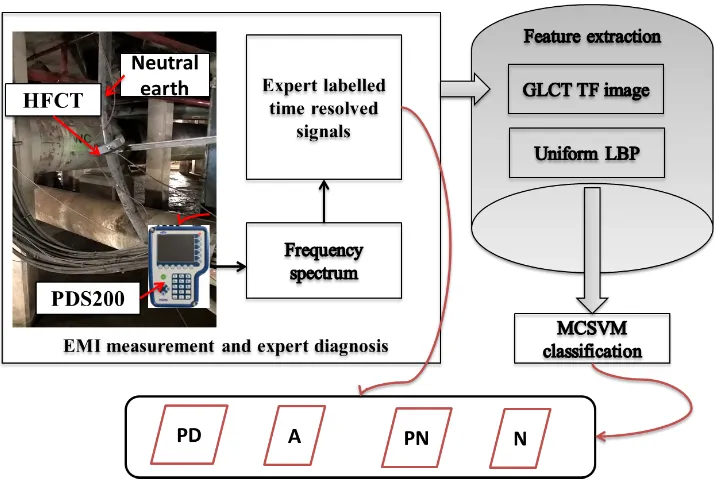
Figure 1: Framework of the proposed method for Electromagnetic Interference (EMI) analysis using High-Frequency Current Transformer (HFCT) and Partial Discharge (PD) Surveyor 200 (PDS200), discharge sources classification results are compared against experts’ labelling of the sensed signals: PD, Arcing (A), Process Noise (PN) and Corona (C).

EMI technique providing the frequency spectrum from which experts select and label time resolved signals; 2) the time series are segmented into smaller signal chunks of 4000 samples for simple computation of the TF image and in order to feed the classifier with more instances for an improved training phase; 3) TF image of each segment is obtained using GLCT; 4) a histogram of uniform LBP is extracted as a feature vector of the TF image; 5) the feature vector is fed into the MCSVM classifier along with the relevant expert label.

2.2. EMI monitoring

allows capturing EMI time-domain signals at the frequencies of interest for au-dio analysis by EMI experts with the aim of identifying the event [18]. Such identification is based on previously accumulated experience of fault monitoring and forensic confirmation based on audio analysis. This approach is limited as it relies totally on the availability of experts with such knowledge. This paper attempts to overcome this limitation by using the expert’s knowledge as a la-belling method and a foundation to an intelligent pattern recognition algorithm for automatic fault classification of EMI time resolved data. The approach is to employ feature extraction and classification techniques which are described in the following section.

3. Feature Extraction algorithm

In this section the mathematical theory of GLCT and uniform LBP is pre-sented.

3.1. General Linear Chirplet Transform (GLCT)

GLCT was proposed by Yu and Zhou to analyse time-varying Instantaneous Frequency (IF) signals and to overcome some limitations in STFT and the Lin-ear Chirplet Transform (LCT) [30]. This includes higher energy concentration and better resolution on the T-F domain with reduced cross-term interference, superior ability to analyse non-linear single and multi-component signals, and finally more tolerance against noise [35].

The mathematical framework of GLCT is described as follows. First, de-noted in Equation 1 is a time-varying IF signal with amplitude A(t) and IF

φ(t)

x(t) =A(t).eiRφ(t)dt. (1) Given a short time τ and an instantaneous time t0, the IF can be a linear equation that is developed by Taylor expansion as follows.

φ(τ) =φ(t0) +φ0(t0)(τ−t0). (2)

By applying a short windoww(τ−t0) tox(τ) atφ(t0), then calculating the FT of their product gives:

|S(φ(t0))|=|

Z +∞

−∞

w(τ−t0).x(τ).e−iφ(t0)τdτ|.

=|

Z +∞

−∞

w(τ−t0).A(τ).eiφ(t0)τ+iφ0(t0)(τ−t0)2/2

.e−iφ(t0)τdτ|.

(3)

By performing some mathematical manipulations, Equation 3 is simplified to obtain Equation 4.

|S(φ(t0))|=|

Z +∞

−∞

It is observed that there is a modulated element eiφ0(t0)(τ−t0)2/2 which causes dispersion of the energy around IF and higher concentration of harmonics on the T-F domain. In order to remove the modulated element, a demodulated factor is introduced to the general STFT in Equation 5 to obtain the new formulation in Equation 6. The latter includes the chirp rate “c”space which aims to rotate the signal by a degree of arctan(c) in the TF space.

S(t0, ω) =

Z +∞

−∞

w(τ−t0).x(τ).e−iωτdτ. (5)

S(t0, ω) =

Z +∞

−∞

w(τ−t0).x(τ).e−iωτ.e−ic(t0)(τ−t0)2/2dτ. (6)

The new STFT amplitude can hence be calculated as follows.

|S(t0, φ(t0))|=|

Z +∞

−∞

w(τ−t0).x(τ).e−iφ(t0)τ

.e−ic(t0)(τ−t0)2/2dτ|

=|

Z +∞

−∞

ei(φ0(t0)−c(t0))(τ−t0)2/2

.w(τ−t0).A(τ)dτ|.

(7)

The inconvenience of this demodulated solution is that it is difficult to pre-define the factor accurately because the IF characteristics of a signal cannot be estimated a priori. A possible approach is to employ a series of discrete demodulated factors to estimate the optimum factor given by:

S(t0, ω, c) =

Z +∞

−∞

w(τ−t0).x(τ).e−iωτ.e−ic(τ−t0)2/2dτ. (8)

This way, for each (t0, ω) if the discrete factor corresponds to the modulated factor, then the T-F around the signal’s IF will have high energy concentration and maximum amplitude. Thus based on this amplitude, the best parameter “c”can be calculated as:

c0 =argmax

c |S(t

0_{, ω, c)|. (9)}

Finally, GLCT can be computed as follows.

GS(t0, ω) =S(t0, ω, c0). (10) Note that Equation 8 is equal to LCT, whenc= 0, from which GLCT (Equation 10) is derived. The demodulated factor results in a rotation on the TF by an angle of arctan(−c). This is characterised by a rotating parameterα∈[−π

2,

π

2]

which is defined in Equation 11 for a known sampling timeTsand frequencyFs

of a signal.

α= arctan(2Ts

Fs

Assume thatαhas N values which divide the T-F domain into N+1 segments evenly as:

α=−π

2 +

π N+ 1,−

π

2 + 2π N+ 1...,−

π

2 +

N π

N+ 1. (12) Then, this N parameter is what differentiates GLCT from STFT. However, whenN= 1 then GLCT yields to STFT. The recommendedN value by authors in [30] lies between 5 to 10. They demonstrated that higher values do not reduce errors or cross terms interference any further, however computation is increased which is not desired in signal processing implementations. An example non-stationary signal is provided in Figure 2 from which the TF image was calculated using STFT and GLCT algorithms as illustrated in Figures 3 and 4 respectively. It is observed that GLCT extracts the IF with better resolution and concentration than STFT.

Figure 2: Example non-stationary Signal

Figure 3: STFT image of the example non-stationary Signal

Figure 4: GLCT image of the example non-stationary Signal

3.2. Local Binary Pattern (LBP)

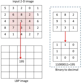
LBP exploits the image pixels by comparing their values to those of neigh-bouring ones and uses the result as binary number to labels each pixel [36]. Figure 5 illustrates an example which explains the mathematical concept of coding a 2-D image to LBP. Suppose that ”C” is the centre pixel and ”P” the neighbours equally spaced from ”C” at distance ”R” (see Figure 6), the joint difference distribution is calculated as:

Figure 5: LBP image encoding of a 2-D image

T ≈(g0−gC, ..., gP−1−gC) (13)

wheregC andg0 togP−1are the Gray level intensity of the centre pixelC and

Figure 6: LBP histogram representation of an image

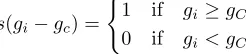
s(gi−gc) = (

1 if gi≥gC

0 if gi< gC

whereT can be written in Gray scale format T ≈(s(g0−gC), ..., s(gP−1−gC)),

for the neighbours indexi= [0, P]. Finally an LBP value for each pixelC, with the coordinates (xC,yC); xC ∈ {0, ..., N−1},yC∈ {0, ..., M−1} on theNxM

image, is calculated as follows:

LBPP,R(xC,yC) =

P−1

X

i=0

s(gi−gC)2i. (14)

This results in a unique value 0≤C0 _≤2i_{. A histogram with size P}2 _{of LBP}

values is created producing a vector of 256 descriptive features for 8 neighbours. Figure 6 illustrates how this is derived. It was recommended in [37] to consider only the possible uniform values in the histogram. They also suggested to implement LBP with 2 points distance. This implies a reduction of the feature vector dimension from 256 to 59 and improvement in computation. An LBP is uniform if the binary code has a maximum of two 01 or 10 transitions. For instance, the LBP in Figure 5 for example is uniform. A non uniform LBP would be 10010010. Non-uniform LBP descriptors are considered noisy and useless for classification, whereas the uniform ones provide information on uniform regions, edges and corners in the image [38]. This property could be exploited to extract such information from the TF behaviour of the discharge sources. A deeper explanation of uniform LBP can be found in [39]. Thus, uniform LBP with the parametersR= 2 andP = 8 neighbours are chosen in this work.

4. Support Vector Machine(SVM) and Multi-Class SVM(MCSVM)

Figure 7: SVM linear separation

Figure 8: SVM linear space mapping using RBF kernel function

the RBF kernel, withσ= 0.5, which is defined as follows.

K(xi, xj) =e−

||xi−xj||2

2σ2 (15)

whereσis the width of the RBF function.

The mathematical theory of SVM can be described as follows: Letxi be the

data input andyi the associated labels in that i= 1,2, ...Lis the data sample

number. Let’s assume that the data points belong to two classes “1”and “−1”. Each data point is put into a feature space which is separated by a hyperplane with the basic geometric equation:

f(x) =w.x+b= 0 (16)

wherebis a scalar and wis an L-dimensional vector which plays an important role in determining the hyperplane position. The hyperplane will pass by the origin ifb= 0. Otherwise, the margin will be created or increased. Equation 17 defines the hyperplane of the first class and Equation 18 defines the hyperplane of the second one.

w.x+b= 1. (17)

w.x+b=−1. (18)

Through geometric manipulations, the distance between the two hyperplanes can be obtained as _|w2_|. The margin width can be maximised by minimising|w|

which brings in the criteria: w.xi+b≥1 and w.xi+b ≥ −1 for the first and

second class respectively. This will ensure that the points from each class do not surpass the hyperplanes which are also called support vectors. The instances that fall on the hyperplanes are called support vectors. The hyperplane is calculated by solving the optimisation problem in Equation 19, while taking into consideration two main parameters: the noise slack variable ζi and the

min1

2||w||

2_+C

M X

i=1

ζi. (19)

Subject to

(

yi(wT.xi+b)≥1−ζi

ζi≥0, i= 1, ..., M

whereζidefines the range to which the samples exceed the margin andCstates

the trade-off between classification error, which results from the training phase, and maximisation of the margin. Equation 19 is transferred to Lagrangian optimisation problem. Further details and explanation can be found in [44]. This inserts anαi parameter which expresses w in solving Equation 19. The

solution results in a non-linear decision function which is defined in Equation 20.

f(x) =sign(

M X

i,j=1

αiyi(xixj) +b). (20)

The challenges that can be faced by the SVM learning process with high dimen-sion feature space are data over-fitting and computational errors. Over-fitting can be tackled by implementing a kernel function which performs a dot product of the feature space i.e. K(xi, xj) = (ΦT(xi).Φ(xj)), where the definition of

this function is presented in [40] . This is similar to the case of non-linear map-ping as discussed earlier. A non-linear vector function Φ(x) = (φ1(x), ..., φl(x))

with feature space of dimensionl is implemented and the decision function in Equation 20 is reformulated to:

f(x) =sign(

M X

i,j=1

αiyi(ΦT(xi).Φ(xj)) +b). (21)

SVM is a binary classifier which means it can deal with only two different classes. In this paper as we seek to classify more than two events. MCSVM is implemented to overcome this issue by employing the One-Against-One (OAO) approach where k(k−1)/2 models are built and each one is trained on two classes,pandq, as a normal binary classifier. The testing is performed using a ”Max Win” voting approach. If the test instance is near thepthclass then the vote for this class is incremented by one. The test instance is classified in the class which obtains the highest vote [45].

5. Application

5.1. EMI data description

frequency measurements to the international standard CISPR16 for EMI filter types. The PDS200 is a PD surveyor device which detects and analyses Radio Frequency Interference (RFI) in addition to EMI radiations. The device pro-vides the frequency spectrum of the captured signals using quasi-peak detector. The latter is fast enough to measure the discharges intensity, unlike other de-tectors (e.g. AM rms) used in RFI testing [27]. The PDS200 is a radio receiver which captures EMI radiations in the range of 0 to 100MHz. The selected fre-quency of interest within this span demodulates, by means of AM demodulation, the signal which is sampled at 24 kHz. The PDS200 looks at signals based on the CISPR16 bandwidths (e.g. 9kHz, 120kHz) and moves through the frequency spectrum making appropriate power filtered response measurements at each fre-quency. For time domain signals the instrument permits any frequency between 150kHz to 100MHz to be selected e.g. where the maximum envelope energy exists. It then makes a slower filtered response measurement which is sampled at 24kHz.The time resolved signal can be retrieved for further analysis from a selection of significant peaks in the frequency spectrum. Figure 9 illustrates an example of the frequency spectrum obtained from a generator by the PDS200 quasi-peak detection and Figure 10 shows an example time series signal which was retrieved at 7MHz, measured from the generator in microvolts.

Figure 9: EMI frequency spectrum

Figure 10: Time series signal captured at 7MHz

Table 1: faults’ labels

Fault Label

Arcing A

Corona C

Data Modulation D

Exciter E

minor Sparking mS

Noise N

Random Noise RN

Partial Discharge PD

Table 2: Detected faults in each site

Site Assets Conditions

1 Unit 3 Background stair rail, Generator 2, Generator Unit 3,

Unit 3 IPB Yellow Phase PD, RN, PN, mPD, C, N

2 Generator Step-Up (GSU) 3, Gas Turbine 1 A/B/C Phase, Gas Turbine 2 A/B/C Phase, Gas Turbine 2 A Phase Coupler, Steam

Turbine Generator A/B/C Phase, IPB, Station Transformer PD, E, PN, D

3 Gas Turbine 2, IPB, Steam Turbine Generator PD, E, PN

4 Boiler Feed Pump, Salt Water Pump, Steam Turbine Generator 3 mS, D, RN, PD, A

5 Generator, GSU PD, E

6 Transformer 1B/2B RN, D, PD

7 GSU 8 PD, PN, E

8 Unit (Auxiliary) Transformers 1a, 1b, 2a, and 2b RN, D, E, PD, mS

9 Auxiliary Transformer, GSU, Steam Turbine Generator PD, E

10 Generator Unit 1, 2 and 3 PN, E, PD

and reduced discharge level. The work in this paper is about classification not trending. However, once the fault is classified the PDS200 can permit trending [17] [46] to be undertaken e.g. repetition rate, magnitude level increases etc. so the severity can then be evaluated and trended. As the PDS200 measures selected frequencies using CISPR16 bandwidths the signals don’t calibrate in the same way as conventional PD measurements.

(a) (b)

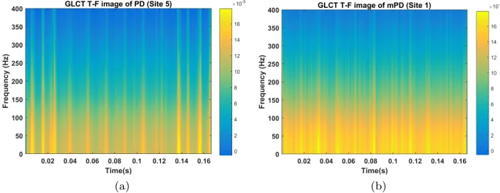
Figure 11: TF image for (a) PD (b) minor PD.

5.2. Application and results

between them is obvious. Similar differences are also observed between the dif-ferent events, giving a motivation to use the GLCT image along with LBP as features to help event classification. In order to reduce the feature dimension and redundant information, uniform LBP withR= 2 andP= 8 was computed to extract the pattern of each TF image. This provided a total of 60 instances per signal with a feature vector length of 59. The feature vectors are then im-plemented in the MCSVM OAO algorithm for classification. The classifier is trained and tested using a ten-fold hold-on cross validation method where 10% of the total data set is kept for testing and the rest is used for training. A different data training/testing set is selected in ten iterations and the average of the resulting accuracies from each iteration is considered as the total classifi-cation accuracy. For results consistency, this simulation was performed several times with differentN parameter values of the GLCT (N= [1−15]), where an improvement of only 1 to 2% in classification accuracy was obtained forN ≥3.

5.3. Results

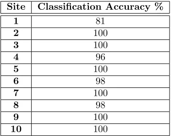
The classification performance is evaluated and presented in terms of accu-racy percentage and confusion matrix. The latter aids to visualize the classifica-tion performance in terms of the true and predicted class of each event. Detailed explanation of the confusion matrix can be found in [47]. The classification was performed in two different scenarios as follows.

Table 3: Classification accuracy within each site

Site Classification Accuracy %

1 81

2 100

3 100

4 96

5 100

6 98

7 100

8 98

9 100

10 100

5.3.1. Case 1

containing two or up to three events have the best classification accuracy. The latter is degraded as the number of events per site increases. In order to further investigate the results where accuracy of 100% was not achieved, confusion ma-trices between the different events were plotted in Figures 12 to 15 for Sites 1, 4, 6 and 8 respectively. Overall, classification confusions were observed between PD, mPD, RN and N in Site 1 (Figure 12). The major confusion was observed between mPD and PD with 44.4%. This could be because PD and mPD are the same fault type, thus a second stage analysis is required. For this concern, it may be possible to use other aspects of the signals to discriminate them and this is something which will be looked at in the future to improve classification. In Site 4 (Figure 13), PD has minor confusion (3.3%) with mS, A has small confusions with PD (1.4%) and mS (4.2%) and finally RN has small confusion with A (2.4%). In Site 6 (Figure 14), PD has confusion of 16.7% with RN and RN has a small confusion (3%) with D. Finally, only one confusion was observed in Site 8 (Figure 15) which is 2.8% between PD and mS.

Figure 12: Confusion matrix of Site 1

5.3.2. Case 2

In this case the MCSVM was trained/tested using the ten fold cross-validation approach on a dataset that contains a mix of all the data events (7) acquired from all sites (10). A classification accuracy of 87% was achieved in this case. The drop in accuracy is realistic as the MCSVM task becomes more challenging when classifying a larger number of events. However, this may be regarded as a good performance. The confusion matrix of all events across the 10 sites is pre-sented in Figure 16 to better understand and justify the obtained classification results. As seen, mS is the event which has the most confusions with PD, D, E, and A. PD and RN have small confusions with the other classes particularly PN, N, mPD, D, A and mS. A has confusions with PD and PN only and E has confusion of 1% with PD.

Figure 13: Confusion matrix of Site 4

Figure 15: Confusion matrix of Site 8

classification of single labelled EMI signals. This may be exploited for automatic condition assessment of high voltage assets or power plants. However, practical implementation or instrumentation of this approach may be challenging as it is heavy in computation and thus requires powerful and sophisticated computers.

6. Conclusions

This paper introduces a highly accurate feature extraction and classification algorithm that is built upon expert knowledge of electrical machine condition assessment using EMI diagnosis technique. The feature extraction was imple-mented to retrieve the complex difference between the time series signals of each discharge source and in order to facilitate the classification process. Ex-cellent classification accuracy was achieved within each site as well as across all the different sites. The authors plan to investigate other aspects of the signal to address the confusion issue between PD and mPD. As for now, this work may contribute in the development of an automatic condition monitoring in-strument in the future for industrial application. However, computation cost of the algorithm should be taken into account. Moreover, it would be desirable to gain more confidence in the classification by training the algorithm with more instances of EMI events.

References

[1] Y. Tian, P. Lewin, A. Davies, Comparison of on-line partial discharge de-tection methods for hv cable joints, IEEE Transactions on Dielectrics and Electrical Insulation 9 (2002) 604–615.

[2] L. Satish, W. S. Zaengl, Artificial neural networks for recognition of 3-d partial discharge patterns, IEEE Transactions on Dielectrics and Electrical Insulation 1 (2) (1994) 265–275.

[3] F. Kreuger, Industrial High Voltage: 4. Coordinating, 5. Testing, 6. Mea-suring, Delft University Press, Delft, The Netherlands, 1992.

[4] G. Robles, E. Parrado-Hern´andez, J. Ardila-Rey, J. M. Mart´ınez-Tarifa, Multiple partial discharge source discrimination with multiclass support vector machines, Expert Systems with Applications 55 (2016) 417 – 428.

[5] J. E. Timperley, J. M. Vallejo, Condition assessment of electrical apparatus with emi diagnostics, IEEE Transactions on Industry Applications 53 (1) (2017) 693–699.

[7] M. Wu, H. Cao, J. Cao, H. L. Nguyen, J. B. Gomes, S. P. Krishnaswamy, An overview of state-of-the-art partial discharge analysis techniques for condition monitoring, IEEE Electrical Insulation Magazine 31 (6) (2015) 22–35.

[8] M. Mondal, G. Kumbhar, Detection, measurement, and classification of partial discharge in a power transformer: Methods, trends, and future re-search, IETE Technical Review 0 (0) (2017) 1–11.

[9] T. Hong, M. T. C. Fang, Detection and classification of partial discharge using a feature decomposition-based modular neural network, IEEE Trans-actions on Instrumentation and Measurement 50 (5) (2001) 1349–1354.

[10] S. C. Oliveira, E. Fontana, Optical detection of partial discharges on in-sulator strings of high-voltage transmission lines, IEEE Transactions on Instrumentation and Measurement 58 (7) (2009) 2328–2334.

[11] I. B´ua-N´u˜nez, J. E. Posada-Rom´an, J. Rubio-Serrano, J. A. Garcia-Souto, Instrumentation system for location of partial discharges using acoustic detection with piezoelectric transducers and optical fiber sensors, IEEE Transactions on Instrumentation and Measurement 63 (5) (2014) 1002– 1013.

[12] W. M. F. Al-Masri, M. F. Abdel-Hafez, A. H. El-Hag, A novel bias detection technique for partial discharge localization in oil insulation system, IEEE Transactions on Instrumentation and Measurement 65 (2) (2016) 448–457.

[13] W. M. F. Al-Masri, M. F. Abdel-Hafez, A. H. El-Hag, Toward high-accuracy estimation of partial discharge location, IEEE Transactions on Instrumentation and Measurement 65 (9) (2016) 2145–2153.

[14] N. D. Jacob, W. M. Mcdermid, B. Kordi, On-line monitoring of partial discharges in a hvdc station environment, IEEE Transactions on Dielectrics and Electrical Insulation 19 (3) (2012) 925–935.

[15] G. Robles, M. S´anchez-Fern´andez, R. A. S´anchez, M. V. Rojas-Moreno, E. Rajo-Iglesias, J. M. Mart´ınez-Tarifa, Antenna parametrization for the detection of partial discharges, IEEE Transactions on Instrumentation and Measurement 62 (5) (2013) 932–941.

[16] J. E. Timperley, Detection of insulation deterioration through electrical spectrum analysis, in: 1983 EIC 6th Electrical/Electronical Insulation Con-ference, Chicago, USA, 1983, pp. 60–64.

[18] J. E. Timperley, Audio spectrum analysis of emi patterns, in: 2007 Elec-trical Insulation Conference and ElecElec-trical Manufacturing Expo, Nashville, USA, 2007, pp. 39–41.

[19] T. K. Abdel-Galil, R. M. Sharkawy, M. M. A. Salama, R. Bartnikas, Par-tial discharge pattern classification using the fuzzy decision tree approach, IEEE Transactions on Instrumentation and Measurement 54 (6) (2005) 2258–2263.

[20] K. Yanbin Xie, J. Tang, Q. Zhou, Feature extraction and recognition of uhf partial discharge signals in gis based on dual-tree complex wavelet transform, European Transactions on Electrical Power 20 (5) (2010) 639– 649.

[21] D. Evagorou, A. Kyprianou, P. L. Lewin, A. Stavrou, V. Efthymiou, A. C. Metaxas, G. E. Georghiou, Feature extraction of partial discharge signals using the wavelet packet transform and classification with a probabilistic neural network, IET Science, Measurement Technology 4 (2010) 177–192.

[22] R. Hussein, K. B. Shaban, A. H. El-Hag, Robust feature extraction and classification of acoustic partial discharge signals corrupted with noise, IEEE Transactions on Instrumentation and Measurement 66 (3) (2017) 405–413.

[23] J. E. Timperley, D. Buchanan, J. M. Vallejo, Electric generation condition assessment with electromagnetic interference analysis, IEEE Transactions on Industry Applications PP (99) (2017) 1–1.

[24] I. Mitiche, G. Morison, A. Nesbitt, P. Boreham, B. G. Stewart, Clas-sification of partial discharge emi conditions using permutation entropy-based features, in: 2017 25th European Signal Processing Conference (EU-SIPCO), 2017, pp. 1375–1379.

[25] C. V. Maughan, Electromagnetic interference (emi) testing of electrical equipment, in: 2011 Electrical Insulation Conference (EIC)., 2011, pp. 340– 344.

[26] J. Stein, Assessment of partial discharge and electromagnetic interference on-line testing of turbine-driven generator stator winding insulation sys-tems,www.rpi.edu/ nelsoj/epri.pdf(March 2003).

[27] J. E. Timperley, Comparison of pda and emi diagnostic measurements [for machine insulation], in: Conference Record of the the 2002 IEEE Interna-tional Symposium on Electrical Insulation, Boston,USA, 2002, pp. 575–578.

[29] M. Chai, Y. H. M. Thayoob, P. Ghosh, A. Z. Sha’ameri, M. A. Talib, Identification of different types of partial discharge sources from acoustic emission signals in the time-frequency representation, in: Power and Energy Conference, 2006. PECon ’06. IEEE International, Putrajaya, Malaysia, 2006, pp. 50–585.

[30] G. Yu, Y. Zhou, General linear chirplet transform, Mechanical Systems and Signal Processing 70–71 (2016) 958 – 973.

[31] N. Agera, S. Chapaneri, D. Jayaswal, Exploring textural features for au-tomatic music genre classification, in: 2015 International Conference on Computing Communication Control and Automation, 2015, pp. 822–826.

[32] W. Yang, S. Krishnan, Combining temporal features by local binary pat-tern for acoustic scene classification, IEEE/ACM Transactions on Audio, Speech, and Language Processing 25 (6) (2017) 1315–1321.

[33] M. Esfahanian, H. Zhuang, N. Erdol, Using local binary patterns as features for classification of dolphin calls, The Journal of the Acoustical Society of America 134 (1) (2013) EL105–EL111.

[34] T. Ahohen, A. Hadid, M. Pietikainen, Face recognition with local binary patterns, in: 8th European Conference on Computer Vision, Prague, Czech Republic, 2004, pp. 469–481.

[35] Y. Huang, X. Zheng, Spectral decomposition using general linear chirplet transform, in: SEG International Exposition and Annual Meeting, Hous-ton, USA, 2017, pp. 2164–2168.

[36] T. Ojala, M. Pietikainen, T. Maenpaa, Multiresolution gray-scale and rota-tion invariant texture classificarota-tion with local binary patterns, IEEE Trans-actions on Pattern Analysis and Machine Intelligence 24 (7) (2002) 971–987.

[37] Y. Costa, L. Oliveira, A. Koerich, F. Gouyon, J. Martins, Music genre clas-sification using{LBP} textural features, Signal Processing 92 (11) (2012) 2723 – 2737.

[38] D. Battaglino, L. Lepauloux, L. Pilati, N. Evans, Acoustic context recog-nition using local binary pattern codebooks, in: 2015 IEEE Workshop on Applications of Signal Processing to Audio and Acoustics (WASPAA), New York, USA, 2015, pp. 1–5.

[39] M. Topi, O. Timo, P. Matti, S. Maricor, Robust texture classification by subsets of local binary patterns, in: in Proceedings of the 15th International Conference on Pattern Recognition, Barcelona, Spain, 2000, pp. 947–950.

[41] C. Bishop, Pattern Recognition and Machine Learning, Springer, Cam-bridge, UK, 2006.

[42] B. R. K. N. S. G. Lesniak JM., Hupse R., Comparative evaluation of sup-port vector machine classification for computer aided detection of breast masses in mammography, Physics in Medicine and Biology 57 (2012) 2560 – 2574.

[43] M. Boardman, T. Trappenberg, A heuristic for free parameter optimization with support vector machines, in: International Joint Conference on Neural Networks, Vancouver, Canada, 2006, pp. 1337–1344.

[44] A. Widodo, B.-S. Yang, Support vector machine in machine condition moni-toring and fault diagnosis, Mechanical Systems and Signal Processing 21 (6) (2007) 2560 – 2574.

[45] C.-W. Hsu, C.-J. Lin, A comparison of methods for multiclass support vector machines, IEEE Transactions on Neural Networks 13 (2) (2002) 415–425.

[46] J. E. Timperley, Generator condition assessment through emi diagnostics, in: ASME 2008 Power Conference, 2008, pp. 349–354.