Energy System Planning and Control
Wai Keung Terrence Mak
A thesis submitted for the degree of
Doctor of Philosophy of
The Australian National University
P
hD thesis, is an important milestone in one’s life. It records someone’s time, ina foreign country with kangaroos. It marks the progress of a research journey. It discloses many excitements and joys of a research program. In the end, it declares the birth of an academic researcher.The long journey as a research student started as early as in 2009, when he was pursuing his M.Phil degree in Chinese University of Hong Kong. With the support from his former supervisor, he took the courage and flied himself to Australia in 2013 to start his PhD study in University of Melbourne and worked in the NICTA Victoria laboratory. In Melbourne, he met his supervisor and later transferred with him to the Australian National University in 2014, while working in the NICTA Canberra laboratory. Throughout the journey, there are many people, directly or indirectly, supporting his life and studies.
I would like to thank my PhD and post-doc supervisor Prof. Pascal Van Hentenryck for his endless support and supervision. He is always optimistic in research, and an exciting professor to work with. I would also like to thank my other academic advisors: Prof. Sylvie Thiebaux, Prof. Peter Stuckey, Dr. Hassan Hijazi, and Dr. Carleton Coffrin, and our collaborators: Prof. David Hill, Prof. Ian Hiskens, Prof. Yunhe Hou, Prof. Tao Liu, Dr. Anatoly Zlotnik, and Dr. Russeull Bent for their constructive ideas and helpful guidance. They help me a lot to strengthen my academic knowledge. They also assist me in exploring new research areas and directions. I would also like to thank all of my colleagues, lab-mates, and friends for supporting my research and life. They include, but are not limited to: Prof. Lexing Xie, Prof. Phil Kilby, Dr. Alban Grastien, Dr. Patrik Haslum, Dr. Tommaso Urli, Dr. Victor Pillac, Dr. Andreas Schutt, Dr. Feydy Thibaut, Dr. Caron Chen, Dr. Yury Kryvasheyeu, Dr. Harsha Nagarajan, Dr. Paul Scott, Dr. Andres Abeliuk, Felipe Maldonado Caro, Alvaro Flores, Rodrigo Gumucio, Edward Lam, Boon Ping Lim, Jing Cui, Fazlul Hasan Siddiqui, Alan Lee, Cody Christopher, Ksenija Bestuzheva, Frank Su, Arthur Maheo, Swapnil Mishra, Franc Ivankovic, Carlo Lim, and many more! I would also like to thank my former supervisor Prof. Jimmy Lee for his continuous career guidance, and his son Jasper Lee for discussing ongoing research in constraint programming and algorithmic theory. I also like to thank Justin Yip, a former PhD student of Pascal and a former research visitor of Jimmy, for introducing me to Pascal and guiding/co-authoring with me on my first conference paper in my life. I would also like to thank my current colleagues and students in University of Michigan for spending their time in reading and commenting on the thesis draft. Finally, to all students and researchers, I sincerely wish this thesis would be useful to your research and ongoing studies.
Understanding the physical dynamics underlying energy systems is essential in achieving sta-ble operations, and reasoning about restoration and expansion planning. The mathematics governing energy system dynamics are often described by high-order differential equations. Optimizing over these equations can be a computationally challenging exercise. To overcome these challenges, early studies focused on reduced / linearized models failing to capture system dynamics accurately. This thesis considers generalizing and improving existing optimization methods in energy systems to accurately represent these dynamics. We revisit three applica-tions in power transmission and gas pipeline systems.
Our first application focuses on power system restoration planning. We examine transient effects in power restoration and generalize the Restoration Ordering Problem formulation with standing phase angle and voltage difference constraints to enhance transient stability. Our new proposal can reduce rotor swings of synchronous generators by over 50% and have negligible impacts on the blackout size, which is optimized holistically.
Our second application focuses on transmission line switching in power system operations. We propose an automatic routine actively considering transient stability during optimization. Our main contribution is a nonlinear optimization model using trapezoidal discretization over the 2-axis generator model with an automatic voltage regulator (AVR). We show that con-gestion can lead to rotor instability, and variables controlling set-points of automatic voltage regulators are critical to ensure oscillation stability. Our results were validated against POW
-ERWORLD simulations and exhibit an average error in the order of 10−3 degrees for rotor angles.
Our third contribution focuses on natural gas compressor optimization in natural gas pipeline systems. We consider the Dynamic Optimal Gas Flow problem, which generalizes the Optimal Gas Flow Problem to capture natural gas dynamics in a pipeline network. Our main contribu-tion is a computacontribu-tionally efficient method to minimize gas compression costs under dynamic conditions where deliveries to customers are described by time-dependent mass flows. The scheme yields solutions that are feasible for the continuous problem and practical from an operational standpoint. Scalability of the scheme is demonstrated using realistic benchmark data.
Acknowledgments vii
Abstract ix
1 Introduction 1
1.1 An Overview on Energy Systems . . . 1
1.2 Computational Challenges with System Dynamics . . . 2
1.3 Our Contributions . . . 2
1.3.1 Restoration planning for power systems . . . 2
1.3.2 Transmission line switching for power systems . . . 3
1.3.3 Optimal compression controls for natural gas pipeline systems . . . 3
1.4 Thesis outline . . . 4
1.5 Publication . . . 4
1.6 Government funding acknowledgement . . . 5
2 Background and Related Work 7 2.1 Electrical Power Systems . . . 7
2.1.1 Terminologies and notations . . . 10
2.1.2 Power Flow Problem (PF) . . . 11
2.1.3 Optimal Power Flow Problem (OPF) . . . 14
2.1.4 Applications based on Optimal Power Flow (OPF) . . . 16
2.1.4.1 Power systems restoration . . . 16
Power systems restoration: written plans . . . 17
Power systems restoration planner: knowledge-based systems . 17 Power systems restoration planner: optimization approach . . . 17
2.1.4.2 Transmission line switching . . . 19
Transmission Line Switching Model . . . 21
2.1.5 Power systems stability: Types and characteristics . . . 22
2.1.5.1 Rotor Angle Stability . . . 23
Small-signal Stability . . . 23
Transient Stability . . . 24
Synchronous machine mechanics . . . 24
Synchronizing multiple generators . . . 25
Example scenario: Load variations . . . 26
2.2 Natural Gas Transmission System . . . 27
2.2.1 Terminologies and notations . . . 27
2.2.2 Isothermal gas flow equation . . . 28
2.2.3 Compressor mechanics . . . 30
Modeling discussion . . . 30
2.2.4 Steady-state Gas Flow Equations (Steady GFP) . . . 31
3 An Indirect Stability Approach on Power Systems Restoration 35 3.1 Overview . . . 35
3.2 Our Main Contribution . . . 36
3.3 Prior and Related Work . . . 36
3.4 Transient Modeling on PowerWorld simulator . . . 37
3.5 Topology Changes and Rotor Swings . . . 38
3.6 Power Restoration Ordering Problem with Standing Phase Angle Constraints . 40 3.7 Experimental Evaluation: Case Studies . . . 43
3.7.1 Swing Reduction on Fixed Restoration Order . . . 44
3.7.2 Swing Reduction on Flexible Restoration Order . . . 44
3.7.3 The Impact of SVD Constraints . . . 46
4 A Direct Stability Approach on Transmission Line Switching 49 4.1 Overview . . . 49
4.2 Our Main Contribution . . . 50
4.3 Related Work . . . 52
4.4 Background . . . 52
4.4.1 Generator Model: Swing Equation . . . 52
4.4.2 Generator Model: Classical Swing Model . . . 53
4.4.3 Generator Model: 2-Axis Model . . . 54
4.4.4 Automatic Voltage Regulation Model (AVR) . . . 55
4.5 Finite Difference Method: Trapezoidal Discretization . . . 55
4.5.1 Generator Dynamics: Swing equations . . . 56
4.5.2 Generator Dynamics: Generator Power . . . 57
4.5.3 Generator Dynamics: Stator EMF Dynamics . . . 57
4.5.4 Automatic Voltage Regulator: Exciter . . . 58
4.5.5 Automatic Voltage Regulator: Stabilizer . . . 60
4.5.6 Power Network: AC Power Flow . . . 61
4.5.7 Power Network: Operational Limits . . . 62
4.6 Transient Stable Line Switching . . . 62
4.6.1 Line switching routine with transient stability . . . 63
4.6.2 Transient optimization model . . . 63
4.7 Computational Case Study . . . 64
Evaluation of the TSLS-C Model . . . 65
Evaluation of the TSLS-G Model . . . 66
Evaluation of the TSLS-PSS Model . . . 68
Time horizon: 4 seconds vs 12 seconds . . . 68
Optimization Versus Simulation . . . 70
5 Dynamic Compressor Optimization in Natural Gas Pipeline Systems 79
5.1 Overview . . . 79
5.2 Prior and Related Work . . . 80
5.3 Our Main Contribution . . . 81
5.4 The Dynamic Optimal Gas Flow Problem (DOGF) . . . 83
5.5 Discretization to a Nonlinear Program . . . 85
5.5.1 Trapezoidal Quadrature Rule Approximation . . . 86
5.5.2 Non-dimensional Dynamic Equation with Compressors . . . 86
5.5.3 Pseudospectral Approximation . . . 88
5.5.4 Lumped Element Approximation . . . 89
5.5.5 Constraints and Objective . . . 90
5.6 The Two-Stage Optimization Model . . . 92
5.7 Case Studies . . . 94
5.7.1 Validation . . . 95
5.7.2 Solution Quality and Efficiency . . . 98
5.7.3 Scalability . . . 99
5.8 Extensions & Variants . . . 101
5.8.1 Case 1. . . 103
5.8.2 Cases 2 and 3. . . 105
6 Conclusion and Future Work 109 6.1 Power System Restoration . . . 109
6.2 Transmission Line Switching . . . 109
6.3 Dynamic Compressor Optimization . . . 110
2.1 3-bus power transmission system: 2 generators, 3 transmission lines, 3 buses,
and 2 loads . . . 8
2.2 The classical IEEE-39 bus transmission system [1, 2] ( c1979 IEEE). The im-proved figure ( c2015 IEEE) is copied from the IEEE-PES technical report PES-TR18 (Figure 4.4) [3], which was first appeared from the 39 bus system MATLAB report [4]. . . 9
2.3 The four restoration steps . . . 16
2.4 3-bus power transmission system: Line switching example . . . 21
2.5 Schematic diagram of a synchronous generator from P. Kundur, Power System Stability and Control [5] ( cMcGraw-Hill Education). . . 25
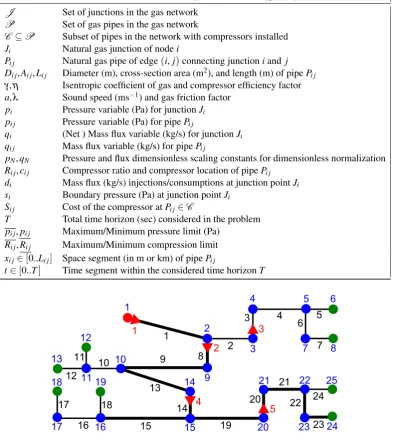
2.6 24-pipe gas system test network used by Zlotnik et. al [6]. . . 28
3.1 The Two Phases of the Restoration Ordering Algorithm. . . 36
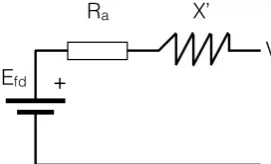
3.2 Circuit diagram of classical generator model . . . 37
3.3 Topology Change Example: Open State (left), Closed State (right). . . 38
3.4 Restoration Case: Generator 1 Rotor Angle (deg) . . . 39
3.5 Removal Case: Generator 1 Rotor Angle (deg) . . . 39
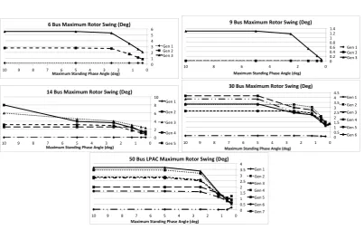
3.6 Maximum Rotor Swing on a Fixed Restoration Order . . . 46
3.7 Maximum Rotor Swing with Optimal Restoration Orderings . . . 46
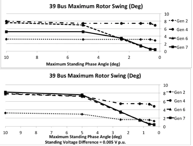
3.8 Maximum Rotor Swing on 39 Bus: SPA Constraints (top), SPA and SVD Con-straints (below) . . . 48
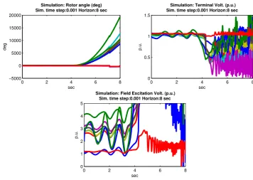
4.1 NESTAnesta_case39_epri__api: Rotor angles (deg, top left), termi-nal voltage (p.u., top right), and field excitation voltage (p.u., bottom) with 88% congestion level for all generators. Each line represents a generator. . . 51
4.2 The control block diagram of our automatic voltage regulator (AVR), with one exciter: SEXS_PTI [7] and one stabilizer: STAB1 [7] . . . 55
4.3 Transient Stable Line Switching Algorithm . . . 62
4.4 TSLS-G Model: Rotor angles (deg), and terminal voltage (p.u.), and excitation field voltage (p.u.) for 85% congestion level (r=1%,γ=0.2%) on opening line (2,25). Each line represents a generator. . . 67
4.5 TSLS-G Model: Rotor angles (deg), and terminal voltage (p.u.), and excitation field voltage (p.u.) for 88% congestion level (r=1%,γ=0.2%) on opening line (16,17). Each line represents a generator. . . 67
4.6 TSLS-PSS Model: Rotor angles (deg), terminal voltage (p.u.), and excitation field voltage (p.u.) with no dispatch change (i.e. r =0%) for opening line (2,25). Left: congestion level 85%, right: congestion level 88%. Each line represents a generator. . . 69
4.7 TSLS-PSS Model: Rotor angles (deg), terminal voltage (p.u.), and excitation field voltage (p.u.) with 1% dispatch change (i.e. r=1%) on 88% conges-tion case for opening line (2,25). Left: 4 seconds horizon, right: 12 seconds horizon. Each line represents a generator. . . 71
4.8 TSLS-PSS Model: terminal voltage (p.u.) and excitation field voltage (p.u.) with 1% dispatch change for opening line (2,25) at congestion level 88%. In-creased simulation time step to 10−4. Each line represents a generator. . . 72
4.9 Error functions on rotor angles (deg), terminal voltage (p.u.), and excitation controls (p.u.) for 88% congestion, withr=0% andγ =0.2%. Discretiza-tion steps size (top to bottom): 0.160s, 0.125s, 0.080s, and 0.040s. Each line represents a generator. . . 74
4.10 Error functions on rotor angles (deg), terminal voltage (p.u.), and excitation controls (p.u.) for (top to bottom) 80%, 85%, and 88% congestion, withr= 0% andγ=0.2%, discretization steps size of 0.080s, and a time horizon of 12
seconds. Each line represents a generator. . . 75
4.11 Optimization solutions on rotor angles (deg), terminal voltage (p.u.), and ex-citation controls (p.u.) for the 115% congestion case, with r =10% and
γ = 0.2%, discretization steps size of 0.080s, and a time horizon of 4
sec-onds. Top: TSLS-G model, Bottom: TSLS-PSS model. Each line represents a generator. . . 78
5.1 A non-smooth solution with trapezoidal time and space discretization. Left to right: Compression ratios; Pressure trajectories (optimization); Pressure tra-jectories (simulation) . . . 92
5.2 24-pipe gas system test network used in the benchmark case study. Numbers indicate nodes (blue), edges (black), and compressors (red). Thick and thin lines indicate 36 and 25 inch pipes. Nodes are source (red), transit (blue), and consumers (green). . . 94
5.4 From top to bottom (Gaslib-40):: Various discretization schemes with: 30 and 150 time points (tp), trapezoidal(TZ) time scheme, trapezoidal(TZ) and lumped element(LU) space scheme, and 10% re-optimization tolerance. From left to right: Optimal control solution; Pressure trajectories from simulation using the controls; Flux trajectories from the same simulation; Relative dif-ference between pressure solution from optimization and pressure trajectories from simulation. . . 101 5.5 Compression ratio solutions for Gaslib-135 case studies, with 22 trapezoidal
(TZ) time points, lumped element (LU) space, and re-optimization tolerance ofr=5%. . . 103 5.6 Optimized demands(kg/s). From left to right: case 1: r=3% and 7%, and
case 3:r=3% and 7%. . . 105 5.7 From top to bottom: Case 1 with 3% and 7% re-optimization tolerance, and
case 2 with 3% and 7% re-optimization tolerance. Both with 50 trapezoidal time point, and lumped space approximation. . . 106 5.8 From top to bottom: Case 3 with 3% and 7% re-optimization, 50 trapezoidal
time point, and lumped space approximation; Case 3 with 3% and 7% re-optimization, 200 trapezoidal time point, and lumped space approximation.
2.1 Nomenclature for power systems networks . . . 8
2.2 OPF solution: Two different congestion settings on four power flow models . . 20
2.3 Nomenclature for natural gas system networks . . . 28
3.1 Line, Load, and Generator Model Parameters . . . 38
3.2 Restoration Case: Settings . . . 38
3.3 Removal Case: Settings . . . 39
3.4 Blackout Size and Convergence Rate for the DC-ROP-SPA. . . 42
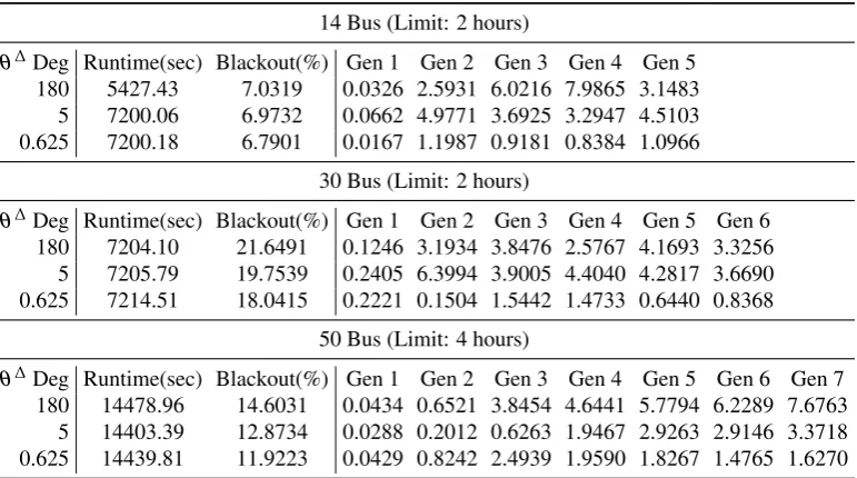
3.5 Runtime & Blackout on a Fixed Restoration Order for Decreasing SPA Values . 45 3.6 Runtime & Blackout on Optimal Restoration Orderings for Decreasing SPA Values . . . 45
3.7 Runtime, Blackout, & Rotor Swings on RAD for Decreasing SPA Values . . . 47
3.8 The 39-Bus New England Test System . . . 47
4.1 Nomenclature for generator models and dynamics . . . 53
4.2 Results for the TSLS-C Model: Dispatch distance (MW/MVAR), Cost Differ-ence ($), and Runtime (sec.). . . 65
4.3 Results for the TSLS-G Model: Dispatch distance (MW/MVAR), Cost Differ-ence ($), and Runtime (sec.). . . 65
4.4 Results for the TSLS-PSS Model: Dispatch distance (MW/MVAR), Cost Dif-ference ($), and Runtime (sec.). . . 68
4.5 Results for the TSLS-PSS Model with T = 12 seconds: Dispatch distance (MW/MVAR), Cost Difference ($), and Runtime (sec.). . . 70
4.6 Results for the Range-Restricted TSLS-PSS Model: Dispatch distance (MW/M-VAR), Cost Difference ($), and Runtime (sec.). . . 72
4.7 Runtime (sec.), Generation cost difference (%), and average errors (deg) . . . . 73
4.8 Runtime (sec.), Generation cost difference (%), and average errors (deg) for 12 seconds horizon optimization at 0.080 seconds time step discretization . . . 73
4.9 Two-axis synchronous generator machine model parameters for the 14-Generator Model benchmark (in system 100 MVA base) . . . 76
4.10 Excitation parameters for the 14-Generator Model benchmark . . . 77
4.11 Power Systems Stabilizer (PSS) parameters for the 14-Generator Model bench-mark . . . 77
4.12 Generation cost parameters for the 14-Generator Model benchmark . . . 78
4.13 Results for TSLS-PSS Model on the 14-Generator Model: Dispatch distance (MW/MVAR), Cost Difference ($), and Runtime (sec.). . . 78
5.1 Aggregated Pressure Bound Violations (vp, psi-days): 24 Pipe. (simulation: 10km space discretization) . . . 95 5.2 Aggregated Pressure Bound Violations (vp, psi-days): 24 Pipe. (simulation:
3km space discretization) . . . 97 5.3 Maximum relative difference (%) in pressure between simulation and
opti-mization: 24 Pipe (simulation: 10km space discretization) . . . 98 5.4 Maximum relative difference (%) in pressure between simulation and
opti-mization: 24 Pipe (simulation: 3km space discretization) . . . 99 5.5 Objective Value (C1) and runtimes on 24 Pipe Network. . . 100 5.6 Objective Value (C1) and runtimes on Gaslib-40 Pipe Network. . . 102
5.7 Maximum relative difference (%) in pressure between simulation and opti-mization: Gaslib-40 . . . 102 5.8 Objective Value (C1) and runtimes on Gaslib-135 Pipe Network. . . 102 5.9 Gas price ($ per 10 kg mass) and optimized demand (kg/s). . . 104 5.10 Objective Value (M1) and runtimes on the maximum contractable throughput
Introduction
1
.
1
An Overview on Energy Systems
Energy transportation systemsare critical for transferring and supplying energy resources to support daily activities in our modern societies. These systems allow us to collect energy re-sources from generation points and transport them to customers. Electricity transmitted by power grids, natural gas flowing in gas pipelines, and water supply traveling through water systems are common types of energy resources and corresponding transportation systems. En-ergy sources are usually not geographically co-located with consumers. Apart from distributed generation such as photovoltaic (PV) systems, most customers stillsolelyrely on energy trans-portation systems for satisfying their needs. A breakdown of such systems not only affects cus-tomers, but could also lead to disastrous events. For instance, on July 30, 2004, a gas pipeline was ruptured and later exploded in Belgium, killing 24 people and injuring over 120 [8]. On August 14-15, 2003, a major power outage occurred in the north-eastern coast of the U.S. and Canada. This event led to a situation where 50 million people were left without power [9].
The question on how to maintain an efficient, stable, and reliable transportation system is thus a critical question. Maintaining the systems in stable operating conditions is a manda-tory requirement. In the U.S., the Federal Energy Regulamanda-tory Commission (FERC) regulates the power grid and issues new regulations/orders [10] to improve and enhance gird stability and efficiency. This translates to different optimization and control problems. For instance, in power (resp., natural gas) systems, the optimal power (resp., gas) flow problem is frequently solved by engineers to find the least cost generation (resp., natural gas) dispatch satisfying cus-tomer demands. To further account for stability and reliability, these energy systems will be routinely checked to ensure a stable control profile exists (e.g., frequency/voltage controls in power systems), bringing the system back to stable conditions when contingencies and faults occur. If no feasible control profile exists, a control problem will then be formulated to find the optimal/feasible control settings. Expansion planning problems are also useful in assisting power/natural gas utilities to understand how to expand and improve their systems. To reduce the computational complexity in solving these optimization and control problems, one pop-ular practice is to ignore the transient dynamics during the optimization phase and consider only steady-state operations. The ignored dynamics will then be later checked via simulation software to ensure that the solutions are acceptable.
1
.
2
Computational Challenges with System Dynamics
Managing energy systems to meet stability and operational conditions requires modeling the physics underlying energy flows and constraints associated with transportation networks. In power systems, the Alternating-Current (AC) power flow equations [5] accurately describe power flows under steady state operations. To model transient dynamics, the classical genera-tor “Swing” model [5] includes 2nd-order differential equations coupled with the non-convex AC power flow equations. The overall formulation can become intractable for optimization. In practice, higher-order differential models are needed to reason on detailed generator be-haviours, resulting in higher-order differential equations for optimization. Similarly, for nat-ural gas, the Euler equations describing the flow of natnat-ural gas along pipes are also nonlinear and differential in nature [11].
To avoid computational intractability, early studies have resorted to using simplified mod-els. In power systems, restoration planning tools usually adopt linearized power flow equations (e.g., the DC power flow equations) with simplified network models and only consider steady-state operations [12, 13, 14]. Detailed network behaviour and transient-steady-states analysis is then conducted by engineers using simulation tools [15, 16, 17]. This approach can lead to sub-optimal plans since multiple iterations between optimization and simulation is needed before converging to a transient-stable solution. Previous research tried to address these issues, e.g., reducing the standing phase angles [18, 19, 20] and directly reasoning on rotor shafts [21]. In early research on transient dynamics, swing equations are modeled using a simplified genera-tor model [5, 1, 22, 23]. Unfortunately, such models fail to capture modern equipments such as automatic voltage and frequency controllers.
1
.
3
Our Contributions
The primary goal of this thesis is to study optimization and planning problems featuring dif-ferential equations describing transient dynamics in energy systems. Three applications are considered in this work. In each case, we demonstrate the issues related to ignoring sys-tem dynamics, before embedding them into novel routines and models enhancing existing ap-proaches. All formulations were validated using well-established simulators, and experimental evaluations were performed on various well-known benchmarks.
1.3.1 Restoration planning for power systems
synchronous generators by over 50%, and 3) by jointly considering both constraints with load pickups and generation dispaches, improvements in rotor swings have negligible impacts on the blackout size. Instead of using repair-based/local-search methods to find stable solutions based on the result from the original optimization routine [24], our model focuses on optimiz-ing all the decisions globally (i.e. holistic optimization).
1.3.2 Transmission line switching for power systems
Our second application focuses on transmission line switching in power system operations. We consider the Optimal Transmission Switching (OTS) [25] problem that searches for the best se-quence of lines to switch off in order to minimize generation costs. The formulation produces an optimal sequence of steady states without guaranteeing transient stability. Our simulation experiments on the IEEE-39 test case indicate the more congested the network is, the more dif-ficult it becomes to ensure transient stability. We propose an automatic routine which actively considers transient stability during optimization. Our key contribution is a nonlinear opti-mization model for Transient-Stable Line Switching (TSLS), using trapezoidal discretization over a 4th-order 2-axis generator model with an automatic voltage regulator (AVR) consisting of an exciter and a stabilizer. The model features two types of control variables: generation dispatches and stabilizer parameters, and its objective function minimizes the rotor angle ac-celerations weighted by time in order to damp and stabilize the system. The key findings are highlighted as follows: 1) the more congested the system is, the more difficult it is to ensure rotor stability, 2) due to the lack of excitation controls in classical swing models, the classical model cannot maintain rotor stability for congested scenarios, 3) the variables controlling the set-points of the exciter and the stabilizer are critical to ensure rotor stability, in particular to maintain (small-signal) oscillation stability, and 4) the TSLS optimization results were vali-dated against POWERWORLD simulations, and exhibit an average error in the order of 10−3 degree for rotor angles.
1.3.3 Optimal compression controls for natural gas pipeline systems
control scheme. The validation process indicates that our optimization scheme produces so-lutions with minimal pressure constraint violations and with physically meaningful mass flow and pressure trajectories that match well with the corresponding simulations. Our method provides a highly accurate solution to a 24-pipe gas benchmark in less than 30 seconds, and demonstrates scalability to three pipeline networks.
1
.
4
Thesis outline
The rest of the chapters are organized as follows. Chapter 2 presents the background material for this thesis, where fundamental equations, concepts, and notations are introduced. Chapter 3 presents our first application on power system restoration planning. Chapter 4 illustrates our second application on power system line switching. Chapter 5 presents our third application on natural gas compression optimization. We then conclude our thesis and discuss our future work in Chapter 6.
1
.
5
Publication
Parts of this thesis were published in various journals/venues. Our work on power system restoration planning was published in:
• [31] Terrence W.K. Mak, Carleton Coffrin, Pascal Van Hentenryck, Ian A. Hiskens, David Hill: Power system restoration planning with standing phase angle and voltage difference constraints. In: Proceedings of the 18th Power Systems Computation Confer-ence (PSCC’14). Wroclaw, Poland (2014)
• [32] Hassan Hijazi, Terrence W. K. Mak, Pascal Van Hentenryck: Power system restora-tion with transient stability.In: Proceedings of the Twenty-Ninth AAAI Conference on Artificial Intelligence (AAAI’15). Austin, Texas (2015)
Our work on power system line switching was published in:
• [33] Terrence W.K. Mak, Pascal Van Hentenryck, and Ian A. Hiskens: A Nonlinear Optimization Model for Transient Stable Line Switching. In: Proceedings of the 2017 American Control Conference (ACC’17). Seattle, USA (2017)
Our work on natural gas compression optimization was published in:
• [34] Terrence W.K. Mak, Pascal Van Hentenryck, Anatoly Zlotnik, Hassan Hijazi, Rus-sell Bent: Efficient dynamic compressor optimization in natural gas transmission sys-tems. In: Proceedings of The 2016 American Control Conference (ACC’16). Boston, USA (2016)
The extended journal version was published in :
1
.
6
Government funding acknowledgement
Background and Related Work
This chapter provides necessary background material for the rest of the thesis. In the first section, we will introduce notations and terminologies for electrical power systems. Power flow equations and the Load/Power Flow Problem will be introduced. We will present the fundamental Optimal Power Flow Problem (OPF), with discussion on two important variants: the original AC-OPF problem, and the simplified DC-OPF problem. We will then describe two important applications: power systems restoration and transmission line switching. Several types of stabilities will be introduced. In particular, we will consider small-signal stability and transient stability. In the second section, we will introduce notations and terminology for describing the natural gas transmission systems. The gas flow equations and the steady-state gas flow problem will then be discussed.
2
.
1
Electrical Power Systems
A traditional electrical power system [5] (also commonly called power grid) consists of three main components: a) generation sources for powergeneration, b) power lines and/or trans-formers for powertransmission, and c) loads for powerconsumption.
Example 2.1.1. Figure 2.1 shows a small example of a power system. The example has two generators for power generation, three transmission lines for power transmission, three buses for power aggregation, and two loads for power consumption, which are commonly drawn as circles, connecting lines, line bars, and arrows respectively. Transmission lines can transmit electric power in any direction. We indicate them as dotted lines if they are opened (i.e., not in service). In this example, if generator 1 is the only operating generator, then power will flow in an anti-clockwise direction (i.e., from Bus 1 to Bus 3, and then from Bus 3 to Bus 2). If generator 2 is the only generator in service, power will flow in a clock-wise direction (i.e., from Bus 2 to Bus 3).
Figure 2.1: 3-bus power transmission system: 2 generators, 3 transmission lines, 3 buses, and 2 loads
Table 2.1: Nomenclature for power systems networks
Nomenclature for power networkP=hN,L,G,Oi
N Set of buses in the power network
N(n)⊆N Subset of neighbouring buses which connect to busn L Set of transmission lines in the power network
G Set of generator machines
G(n) Generators connecting to busn O Set of demands/loads
O(n)⊆O Subset of demands connected to busn b
S,Vb MVA and voltage base for the per unit (p.u.) normalization b
I,Zb,Yb Current, impedance, and admittance base for the per unit (p.u.) normalization pn,qn (Net) Active and reactive power of busn(p.u.)
e
Sn=pn+iqn (Net) Complex power of busn(p.u.)
pnm Active power flow from busntom(p.u.)
qnm Reactive power flow from busntom(p.u.)
e
Snm=pnm+iqnm AC/Complex power flow from busntom(p.u.)
rnm,xnm Resistance and reactance of power line(n,m)(p.u.)
znm=rnm+ixnm Impedance of power line(n,m)(p.u.)
gnm,bnm Conductance and susceptance of power line(n,m)(p.u.)
ynm=1/znm=gnm+ibnm Admittance of power line(n,m)(p.u.)
gn
s Conductance of bus shunts at busn(p.u.)
bn
s Susceptance of bus shunts at busn(p.u.)
lnmc Line charge of line (n,m) (p.u.)
e
Vn,Ien Complex voltage and complex (net) current of busn(p.u.) e
Vn=Vn
∠θn Voltage magnitude & phase angle at busn(p.u.)
Trnm Transformer off-nominal turns ratio (p.u.) from busntom φnm Transformer phase shift from busntom
pnl,q n
l Active and reactive power loads at busn(p.u.)
pn
g,qng Active and reactive generation power at busn(p.u.)
znm On-off line switching variable/parameter
Θnm Total phase difference for line (n,m)
v,v Upper limits and lower limits of a real/complex quantity/variablev v∗ Complex conjugate of a complex quantity/variablev
∆ Discretization time constant (sec)
Figure 2.2: The classical IEEE-39 bus transmission system [1, 2] ( c1979 IEEE). The im-proved figure ( c2015 IEEE) is copied from the IEEE-PES technical report PES-TR18 (Figure
It usually forms the backbone of the overall system and operates at high voltage levels (e.g. 230 kV or above). Thesub-transmission system[5] transmits power received from generators and delivers to distribution systems. Large industrial customers are commonly supplied directly at the sub-transmission level. In some networks, the sub-transmission level is merged with the transmission system. Thedistribution system[5] transmits power to individual customers, and operates at low voltage levels. The primary distribution feeders supply small industrial customers at voltage levels of 4 kV to 35kV, and the secondary distribution feeders connects residential/home customers at common voltages of 100V to 240V. Power systems usually op-erate at a frequency of 50Hz or 60Hz. In terms of topology, distribution systems are mostly radial, with a limited number of cycles in exceptional cases. Transmission systems, e.g., the 10-generator 39-bus IEEE benchmark system [1, 2, 4] shown in Figure 2.2, are commonly found to be more meshed than distribution networks. A meshed network allows the system to be more robust towards faults and loss of equipments, e.g.,N−1 contingency.
2.1.1 Terminologies and notations
In this thesis, we define a power system network P consists of at least the following four sets of equipments: a) a set of busesN, b) a set of transmission lines and transformersL, c) a set of generators G, and d) a set of loadsO. In power systems, symbols are often abused to represent a quantity in different forms. For example,V may be used to represent complex voltage of an equipment at a particular time point, the complex magnitude of an equipment, or a voltage function of an equipment over a series of time points. To avoid confusion be-tween a variable/quantity at a particular time point and its function series, we append ‘()’ to all variables/quantities to represent its function series. In addition, to avoid confusion between complex variablesnfrom its complex magnitude|n|, we add a ‘e’ to the top ofnwhen variable
nmustbe represented in its complex form. We useS,p, andqto denote complex, active, and reactive power respectively. Voltage and current are represented byV andI respectively. We usez,r, andx to represent impedance, resistance, and reactance, andy, g, andbto represent admittance, conductance, and susceptance respectively. Table 2.1 presents a detailed list of notations for each equipment.
We assume power systems parameters and variables are normalized into the per-unit system (p.u.) [5]. In particular, we assume voltages are normalized by the voltage baseVb, and active,
reactive, complex power are all normalized by the MVA power baseSb. The impedance baseZb,
admittance baseYb, and current basebIare defined by the following formula:
b
Z=Vb 2
b
S , Yb=
b
S
b
V2, bI=
b
S
b
V
For simplicity, we assume there is only one generator per bus. Therefore,G⊆NandG(n) =
reverse line(m,n)∈L(vice versa). If there are more than one transmission line (i.e., parallel lines) between a pair of buses, we will use reduction/approximation techniques to compute an equivalent line to replace the originals. We will keep the parallel lines when reducing to one transmission line gives significant differences/errors (e.g., significantly different operational requirements between the parallel lines). To differentiate these parallel lines, we add an extra circuit index numbercto the pair(n,m). LetcN be the maximum number of parallel lines in the corresponding power systems. Transmission lines will be represented by a tuple(n,m,c)∈
L:L⊆N×N× {1, 2,. . .,cN}. Variables and parameterspnm,qnm,Snm,rnm,xnm,Znm,gnm,bnm, Ynm,lnmc ,Trnm,φnm,znm, andΘnmwill be generalized by replacingnmtonmcaccordingly.
2.1.2 Power Flow Problem (PF)
One of the most important and fundamental problems in power systems research is the Power Flow problem, also known as the Load Flow Problem. ThePower Flow Problem (PF prob-lem) [5] in the literature involves the calculation of network power flows (e.g. pnmandqnmof transmission lines) and votages (Vnandθnof buses) of a transmission network subject to
spe-cific terminal/bus conditions or generator configurations. In this problem, all buses will have four variables: the net active power (P), the net reactive power (Q) flowing through the bus, voltage magnitude (V), and voltage angle (θ). Buses will be classified into one of four
differ-ent types: voltage-controlled bus (PV bus), load bus (PQ bus), device bus, or the slack/swing (Vθ) bus. PV buses are typically used to model equipments like generators, synchronous
con-densers, and static var compensators, where the active power (P) and voltages (V) are both specified as input. PQ buses are typically used to model loads, where the active withdrawal (P) and reactive withdrawal (Q) are specified. Device buses are typically used to model buses with devices imposing special boundary conditions/configurations. Power losses in the system are usually not known a priori before solving the PF problem. If we fix all the generators to be PV buses and all the loads to be PQ buses, the system power flow cannot be balanced. In the literature, one classic solution is to set one of the buses with generators to be the slack bus, also known as the swing bus or the reference bus, to automatically balance the power flow. The voltage magnitude (V) and phase angle (θ) of this bus are fixed, and the active (P) and reactive power (Q) are free. This allows the active and reactive power to automatically balance the power flow during the search process to compensate for the unknown power losses. In the lit-erature, the phase angle of the slack bus is usually set to 0. Three methods are typically used to solve the Power Flow problem [5]: 1) Gauss-Seidel Method, 2) Newton-Raphson method, and 3) fast decoupled load flow method. These methods generally solve a set of node equations [5] modeling the law of power flows.
the power flow problem is: e I1 e I2 . . . e Ik =
Y11 Y12 . . . Y1k
Y21 Y22 . . . Y2k
. . .
Yk1 Yk2 . . . Ykk
e V1 e V2 . . . e Vk (I)
whereYnm=
0 ifn6=m,(n,m)6∈L
−ynm ifn6=m,(n,m)∈L
∑
l∈N:(n,l)∈L
ynl ifn=m
e
Inrepresents the complex current of busn∈NandVenis the complex voltage.
This node equation implements the current law in matrix form. Each rowndescribes the current flow balance of busn:
e
In= k
∑
l=1
YnlVel=Yn1Ve1+Yn2Ve2+. . .+YnkVek=
∑
l∈N:(n,l)∈L
[ynl(Ven−Vel)]
The complex matrixY is called the admittance matrix and is extensively used in power systems analysis [5]. Data is usually given in the form of real and reactive power. The current-based equation (I) requires transforming power data/variables to current data/variables. Therefore, the power-based formulation is a preferred alternative. To introduce the power-based formula-tion, we start by introducing the general AC power law:
e
Sn= pn+iqn=VenIe∗n
After substituting with the current-based equations, we have:
pn+iqn=Ven[
k
∑
l=1 YnlVel]∗
LetGandBbe the real and imaginary parts of the admittance matrixY (i.e.Y =G+iB).
pn+iqn=Ven[
k
∑
l=1
(GnlVel+iBnlVel)]∗=Ven
k
∑
l=1
([GnlVel]∗+ [iBnlVel]∗)
=Ven
k
∑
l=1
(GnlVe∗l−iBnlVe∗l) =Ven
k
∑
l=1
We further expand the complex voltage into the polar form.
pn+iqn=Vneiθn
k
∑
l=1
(Gnl−iBnl)Vle−iθl
= k
∑
l=1
(VnVlei(θn−θl)Gnl−
iVnVlei(θn−θl)Bnl)
= k
∑
l=1
VnVl([cos(θn−θl) +isin(θn−θl)]Gnl−i[cos(θn−θl) +isin(θn−θl)]Bnl)
= k
∑
l=1
VnVl(Gnlcos(θn−θl) +Bnlsin(θn−θl) +i[Gnlsin(θn−θl)−Bnlcos(θn−θl)])
We further separate the equations into real and imaginary parts.
pn= k
∑
l=1
VnVl(Gnlcos(θn−θl) +Bnlsin(θn−θl)), and
qn= k
∑
l=1
VnVl(Gnlsin(θn−θl)−Bnlcos(θn−θl))
for alln∈N. The above two equations are generally called theAC power flow equations[5]. We further expand the above two equations on a per-line basis(n,m)∈L. By further expanding the admittance matrixY =G+iB, we obtain [36]:
pn=
∑
m∈N:(n,m)∈Lpnm, where
pnm=gnm[Vn]2−VnVm[gnmcos(θn−θm) +bnmsin(θn−θm)], and
qn=
∑
m∈N:(n,m)∈Lqnm, where
qnm=−bnm[Vn]2−VnVm[gnmsin(θn−θm)−bnmcos(θn−θm)]
The above equations do not model transformers and line charges. To further implement these equipments, we replace the line equation for pnmandqnm[36, 37]:
pnm= g nm[Vn]2
T lnm − VnVm
Trnm [g nm
cos(θn−θm+φnm) +bnmsin(θn−θm+φnm)], and
qnm=−b
nm+lnm c /2 T lnm [V
n]2−VnVm Trnm [g
nmsin(
θn−θm+φnm)−bnmcos(θn−θm+φnm)]
whereφnmdenotes the constant phase shifting angle from busnto busmif transmission line (n,m)has a phase shifting transformer/device. If there are no phase shifting transformers, then
φnm=φmn=0. Phase shifting is directional andφnm=−φmn. Trnmdenotes the off-nominal
flow to generation power, loads, and bus shunts:
pn=png−pln−[Vn]2gns qn=qng−qln+ [Vn]2bns
Solving the Power Flow problem allows us to quickly obtain the steady-state [5] of the network, including power flow on transmission lines, voltage magnitudes and phase angles on buses, with respect to the current generator dispatch and load demands.
2.1.3 Optimal Power Flow Problem (OPF)
In power systems, the cost of generator operations depends on a number of factors, e.g., fuel types and generator scale, and varies from generator to generator. It would be natural for operational engineers to seek for an optimal generation dispatch minimizes generation costs while still satisfying the operational and safety constraints. The Optimal Power Flow Problem (OPF) [38, 39, 40] (or sometimes called Economic Dispatch Problem (ED)) was formulated to achieve this goal. Let pngandqng be the active power dispatch and reactive power dispatch of generatorn, andc(n,pgn) be the cost function evaluating the cost of generatorn at active power pgn. The AC Optimal Power Flow Problem (ACOPF), based on the AC power flow equations, can be formulated as in Model 1. The goal of the problem is to search for a steady state, including voltage solutionsVn,θn, generator dispatch set-pointspng,qng, and power flows pnm,qnm, such that the AC power flow equations are satisfied. We also incorporate the line thermal/power limit constraints as it is a common operational requirement. Since the AC power flow equations are nonlinear and non-convex, the problem is computationally challenging [41]. In the literature, many works [42, 25, 43, 44, 45, 24] use the linearized DC power flow equation [46], simplifying the AC power flow equation by: 1) ignoring the reactive power flow, 2) assuming voltages to be equal to 1 p.u., 3) ignoring resistance in the network, and 4) assuming the phase angle difference is small [36]. Ignoring reactive power flow allows to remove reactive power flows and the corresponding balance equations. By further assuming voltages equal to 1 p.u., we get:
pnm=gnm−[gnmcos(θn−θm+φnm) +bnmsin(θn−θm+φnm)]
By further ignoring resistance assumingg<<b, we obtain a more simplified equation.
pnm=−[bnmsin(θn−θm+φnm)]
Finally, by assuming phase angles are usually small, we can ignore the sine function and all phase shifting actions by transformers / phase shifter.
pnm=−bnm(θn−θm)
Model 1AC Optimal Power Flow Inputs:
P=hN,L,G,Oi Power network input
Variables:
Vn∈[Vn,Vn],∀n∈N Voltage magnitude θn∈(−π,π),∀n∈N Voltage phase angle
pn
g∈[png,png],∀n∈G Active power dispatch
qng∈[qng,qn
g],∀n∈G Reactive power dispatch
pnm∈[pnm,pnm],∀(n,m)∈L Active power flow
qnm∈[qnm,qnm],∀(n,m)∈L Reactive power flow Minimize
∑
n∈G
c(n,png) Subject to:
∑
m∈G(n)
pmg−
∑
m∈O(n)
pml −[Vn]2gns =
∑
m∈N(n):(n,m)∈L
pnm ∀n∈N
∑
m∈G(n)
qmg−
∑
m∈O(n)
qml + [Vn]2bns=
∑
m∈N(n):(n,m)∈L
qnm ∀n∈N
pnm= gnmT l[Vnmn]2−V nVm
Trnm[gnmcos(θn−θm+φnm) +bnmsin(θn−θm+φnm)] ∀(n,m)∈L
qnm=−bnm+lnmc /2
T lnm [Vn]2−V nVm
Trnm[gnmsin(θn−θm+φnm)−bnmcos(θn−θm+φnm)] ∀(n,m)∈L
[pnm]2+ [qnm]2≤ |
g
Snm|2 ∀(n,m)∈L
Model 2DC Optimal Power Flow Inputs:
P=hN,L,G,Oi Power network input
Variables:
θn∈(−π,π),∀n∈N Voltage phase angle
png∈[png,pn
g],∀n∈G Active power dispatch
pnm∈[pnm,pnm],∀(n,m)∈L Active power flow Minimize
∑
n∈G
c(n,png) Subject to:
∑
m∈G(n)
pmg−
∑
m∈O(n)
pml =
∑
m∈N(n):(n,m)∈L
pnm ∀n∈N
pnm=−bnm(θn−θm) ∀(n,m)∈L
Since the DC model does not capture reactive power, it cannot be applied to problems re-quiring reactive power to be modeled explicitly, e.g., capacitor placement problem [51] and voltage stability analysis [5]. Moreover, the accuracy of the model is also an open point of dis-cussion [42, 46, 52, 53, 54, 55]. The question on how to bridge the gap between linearized DC power flow model and non-linear AC power flow models is also an opened path to study, lead-ing to several interestlead-ing recent work: LPAC model [36], QC model [37], and SDP model [56].
2.1.4 Applications based on Optimal Power Flow (OPF)
This section further introduces two power systems applications based on the Power Flow and the Optimal Power Flow problem.
2.1.4.1 Power systems restoration
Power outage may occur when equipments of a power network, e.g., electric buses, transmis-sion lines, transformers, or generators, are faulty / damaged. Users of the faulty power network will usually face phenomena, ranging from a complete blackout, unstable electricity supply, to a short-period power outage. Once power engineers discover that the network is faulty, the restoration process starts immediately. For a severe power system breakdown (e.g., a large electricity blackout), the processes are coarsely divided into three phases [16]:
1. Planning Phase: Devise plans to restart and reintegrate the power supply in the transmis-sion network.
2. Degradation Phase: Perform actions to retain and restore critical sources of power.
3. Restoration Phase: After the system has been stabilized at the degraded state, restore the system to its nominal state.
To successfully complete the above restoration phases, power engineers will usually need to perform four generic tasks (based on Adibi and Fink’s restoration paradigm [15]) as shown in Figure 2.3.
Figure 2.3: The four restoration steps
During the system rebuilding process, engineers may prefer to split the power network into multiple parts/sections, with multiple islands, to speed up the restoration processes [15, 17]. A good restoration plan should be computed to guide the engineers to restore and maintain stability of the system. For example, when we close a line breaker within a partially restored network, we have to make sure the difference between the phase angles across the breaker is small [15, 16]. If the angle is too large and the breaker is closed, stability problems may be observed causing system damage during restorations. In addition, generator stability is also an important topic during load restorations. Coordinating the restorations of the loads to ensure stability is required, and the loading behaviour of generators are necessary to be observed [15, 16]. Connecting a load without enough generation capability will lead to generators tripping off, causing delays to the whole restoration. Coordination between power plants and field operators is required. These two issues were addressed by the first part of our thesis during the optimization of the restoration plans.
Power systems restoration: written plans Devising a plan to efficiently restore a power system is complex. The combinations of possible restoration actions are usually intractable and finding the optimal restoration sequence is computationally hard. Traditionally, power engineers use written restoration plans and procedures as a guidance to perform power systems recovery. These plans and procedures are usually prepared and made based on postulated conditions to give the most effective ways to restore a power system. However, since these written plans are static in nature, they cannot immediately be changed if the actual real-world conditions differ from the postulated conditions. In general, real-world constraints and limiting conditions are hard to predict and it is usually infeasible to enumerate written plans for all possible combinations of conditions. Once power engineers are unable to apply the plan, they are forced to recover the system based on intuition and experience. One main disadvantage of written restoration plans is they are usually written in text. Textual information is intended to be read sequentially. It is hard for power engineers to understand all of the text immediately and perform restorations, particularly under stress and tight time-constraint [17]. Another disadvantage of written plans is that they may not be updated efficiently when the system is changed or upgraded. In a review of 48 major disturbances list, reviewers showed that outdated written plans was the second leading cause of restoration problems [17].
Power systems restoration planner: knowledge-based systems To overcome these disadvantages, knowledge-based expert systems are developed, e.g., Restoration Assistant [57]. These systems usually have the capability to compute and give real-time restoration plans based on actual limitations and conditions. Updating knowledge-based systems to reflect changes in the power system is easier than updating written plans. Once the software is checked and updated, downloading the software to the expert system machines requires far less time than printing written plans.
Model 3DC Restoration Model Inputs:
P=hN,L,G,Oi - Power network input
A=N∪L∪G∪O - The global set of equipments in power systems
D - Set of damaged items
R⊆D - Set of damaged items considered by this algorithm
Variables:(Stepr, 0≤r≤ |R|)
hn(r)∈ {0, 1},∀n∈A - Itemnis going to be repaired (or not) at stepr
kn(r)∈ {0, 1},∀n∈A - Itemnis working/functioning (or not) at stepr
θn(r)∈(−π,π),∀n∈N - Bus phase angle of busnat stepr
png(r)∈[0,pn
g(r)],∀n∈G - Active power by generatornat stepr
pnm(r)∈[pnm(r),pnm(r)],∀(n,m)∈L - Power flow on line(n,m)at stepr
pn
l(r)∈[0,pnl(r)],∀n∈O - Power consumed by loadnat time-stepr Maximize
∑
n∈O
|R|
∑
r=0
pnl(r) (O1)
Subject to:(0≤r≤ |R|)
hn(r) =1, ∀n∈A\D (C2.1)
hn(r) =0, ∀n∈D\R (C2.2)
∑
n∈D
hn(r) =r, (C2.3)
hn(r−1)≤hn(r), ∀n∈D, 1≤r≤ |R| (C2.4)
kn(r) =hn(r), ∀n∈N (C3.1)
km(r) =hm(r)∧hn(r), ∀n∈N,∀m∈G(n)∪O(n) (C3.2)
kl(r) =hl(r)∧hn(r)∧hm(r), ∀(l:n,m)∈L (C3.3)
∑
m∈G(n)
pmg(r)−
∑
m∈O(n)
pml (r) =
∑
m∈N(n):(n,m)∈L
pnm(r) ∀n∈N (C4.1)
¬kn(r)→pn
g(r) =0, ∀n∈G (C4.2)
¬kn(r)→pln(r) =0, ∀n∈O (C4.3)
¬kl(r)→pnm(r) =0, ∀(l:n,m)∈L (C4.4)
kl(r)→pnm(r) =−bnm(θn−θm), ∀(l:n,m)∈L (C4.5)
plans are often criticized due to poor computational efficiency [57, 14]. With advances in hardware performance and optimization algorithms, global approaches are gaining more pop-ularity.
We now explain the variables and constraints in Model 3. The model reasons on|R|+1 steady states with DC power flow approximations, and aims to find the best sequence of steady-states restoring the maximum amount of loads by Objective O1. The model introduces two new types of binary variableshn(r)andkn(r)(with|R|+1 copies) to indicate the status of the equipments in the network. Variablehn(r) is set to 1 (resp. 0) if and only if itemn in step r is repaired (resp. is not repaired), and variable kn(r)is set to 1 (resp. 0) if and only if item nin step r is functioning (resp. not functioning). We defineAto be the union of all buses, loads, and generators. For clarity reasons, we use (l:n,m). In C2.1, we assume all undamaged items to be classified as repaired. In C2.2, we assume all damaged items that are not going to be restored to be classified as not repaired. Constraint C2.3 ensures only one item is being repaired per restoration step. Constraint C2.4 ensures an item being repaired at a particular time-step will be set as repaired in all later time-steps. Constraint C3.1 enforces all repaired buses are functioning immediately. Generators, transmission lines, and loads, all have to be connected to functioning buses. C3.2 and C3.3 restrict these items to be functioning if and only if the associated buses are restored. Constraint C4.1 implements the power flow balance equation. Constraints C4.2, C4.3, and C4.4 ensure that no power is flowing through non-functioning items. The last constraint C4.5 implements the DC power flow equation for functioning lines. Some constraints in Model 3 are logic constraints, and we can linearize them during implementation using the big-M approach [58].
2.1.4.2 Transmission line switching
Transmission line switching is an important control action in electrical power systems, and has generated increasing attention in recent years. Opening and closing transmission lines change the topology of the grid. It is a useful tool to redistribute power flows and change the operational state of the system. Changing the topology could potentially save 10%, or even up to 25% of the economic cost [59, 60, 25]. It also provides opportunities to eliminate congestion and avoid violating operational constraints [61]. Line switching is also an important tool in power systems restoration.
Significant research has been devoted to designing algorithms for Optimal Transmission Switching (OTS) [25]. The goal in OTS is to find the best subset of lines to switch off in order to minimize generation costs. This line of research almost exclusively focuses on analyzing power flow under steady-state before and after the switching. From a mathematical standpoint, the OTS problem is a non-convex Mixed-Integer Non-Linear Program (non-convex MINLP), which is computationally challenging. For this reason, most OTS studies replace the non-convex AC power flow equations by the linear DC power flow equations [25, 62, 63, 64, 65]. This reduces the computational complexity, as the DC-OTS problem can be modeled as a Mixed-Integer Linear Program (MILP). The optimal solution, with integer variables fixed to the optimal values, can be used as a starting solution point and fed into an ACOPF solver to convert into an AC feasible solution. Unfortunately, there is no guarantee that the resulting solution can be transformed into an AC-feasible solution [66, 67]. To overcome this limita-tion, recent work has advocated the use of AC formulations (AC-OTS), or focusing on tighter approximations and relaxations [59, 60, 68].
switch-ing. Without loss of generality, we assume the system is a transmission system withSbbase =
100 MVA andVb = 230kV. In this example, we have three buses, three transmission lines, and
only one load at bus 3 drawing 1 p.u. of active power (i.e. 100MW) and 0 p.u. reactive power. The buses are assumed to be operating within the range of [0.9, 1.1] p.u. voltage magnitude. Line (1,2) and line (2,3) both have negligible resistance and 0.05 p.u. reactance (i.e. z23=z12 = 0 + i 0.05). Line (1,3) has a larger resistance and reactance of both 0.10 p.u. (i.e.z13= 0.10 + i 0.10). For simplicity, we neglect line chargelcnmand bus shuntsgns andbns. There are two generators in the system: one cheap distant generator at bus 1 and one expensive generator at bus 3 located directly on the bus with the load. The cheapest solution is to deliver as much power as possible from generator 1 to avoid using generator 3. For simplicity, we assume the cost function of both generator are linear: c(1,p1g) =p1gandc(3,p3g) =10p3g. We first ignore voltage bounds and line thermal/power limiting constraints. Closing line (2,3) will result in cheaper generation costs of $101 comparing to opening line (2,3) with a cost of $110. Costs in both cases are higher than $100 due to line losses. Adding lines to the network decreases the aggregate network resistance, and therefore resulting in a cheaper generation costs to sup-ply the load. We now consider two congestion cases: 1) imposing a tight thermal/power limit ofgSnm=1 p.u. (MVA) on line (2,3), and 2) reducing the voltage range to [0.98, 1.02] p.u..
Table 2.2 reports the OPF solution with various power flow equations [59]. With the origi-nal AC power flow equations, opening line (2,3) reduces the generation costs by more than 80% for case 1, and increases the generation costs for case 2. The results are further matched by two relaxation techniques: SDP relaxation and QC relaxation (with 5 deg phase bounds). Since the linearized DC power flow model are a coarse approximation omitting reactive power and voltages, the model is not capable to handle voltage congestions in case 2 with significant errors.
Table 2.2: OPF solution: Two different congestion settings on four power flow models
Power Flow Con. case 1 Con. case 2 Model Line open Line close Line open Line close
AC-OPF 110 985 655 102
SDP-OPF 110 972 655 102 QC-OPF (5 deg) 110 772 655 102
Figure 2.4: 3-bus power transmission system: Line switching example
Transmission Line Switching Model LetLsbe the subset of transmission lines(n,m)∈
Model 4AC Optimal Transmission Switching Model Inputs:
P=hN,L,G,Oi Power network input
k Number of lines to be switched off
Variables:
Vn∈[Vn,Vn],∀n∈N Voltage magnitude θn∈(−π,π),∀n∈N Voltage phase angle
png∈[png,pn
g],∀n∈G Active power dispatch
qng∈[qng,qn
g],∀n∈G Reactive power dispatch
pnm∈[pnm,pnm],∀(n,m)∈L Active power flow
qnm∈[qnm,qnm],∀(n,m)∈L Reactive power flow
znm∈ {0, 1},∀(n,m)∈Ls Line switching variable Minimize
∑
n∈G
c(n,png) (O1)
Subject to:
∑
m∈G(n)
pmg−
∑
m∈O(n)
pml −[Vn]2gns =
∑
m∈N(n):(n,m)∈L
pnm ∀n∈N (C2.1)
∑
m∈G(n)
qmg−
∑
m∈O(n)
qml + [Vn]2bns =
∑
m∈N(n):(n,m)∈L
qnm ∀n∈N (C2.2)
∑
(n,m)∈Ls
znm=|Ls| −k (C3.1)
∀(n,m)∈Ls:
pnm=znm× {gnmT l[Vnmn]2−V nVm
Trnm[gnmcos(θn−θm+φnm) +bnmsin(θn−θm+φnm)]} (C3.2)
qnm=znm× {−bnm+lcnm/2
T lnm [Vn]2−V nVm
Trnm[gnmsin(θn−θm+φnm)−bnmcos(θn−θm+φnm)]} (C3.3)
[pnm]2+ [qnm]2≤ |
g
Snm|2×znm (C3.4)
∀(n,m)∈Lr:
pnm=zmn× {gnmT l[Vnmn]2−V nVm
Trnm[gnmcos(θn−θm+φnm) +bnmsin(θn−θm+φnm)]} (C3.5)
qnm=zmn× {−bnm+lcnm/2
T lnm [Vn]2−V nVm
Trnm[gnmsin(θn−θm+φnm)−bnmcos(θn−θm+φnm)]} (C3.6)
[pnm]2+ [qnm]2≤ |
g
Snm|2×zmn (C3.7)
2.1.5 Power systems stability: Types and characteristics
1. Rotor angle stability, with a further sub-classification into:
• Transient stability or large disturbance angle stability and
• Small-signal stability;
2. Voltage stability, with a further sub-classification into:
• Large disturbance voltage stability and
• Small disturbance voltage stability.
In some cases, it is better to classify stability study based on time-range [5, 69]:
1. Short-term stability: seconds scale,
2. Mid-term stability: minutes scale,
3. Long-term stability: hours scale.
In addition, we can also classify stability by their respective control dynamics and processes [69]:
1. Electrical machine and system dynamics,
2. System governing and generation control, and
3. Prime-mover energy supply dynamics and control.
Since our contribution mainly lies on the area of rotor angle stability, we will introduce rotor angle stability, including the two sub-classes: transient stability and small-signal stability, in below subsections.
2.1.5.1 Rotor Angle Stability
Rotor angle stabilitystudy (sometimes called rotor angle study/rotor study) involves the inves-tigation of electromechanical oscillations in power systems, primarily due to the rotor oscilla-tions in synchronous generator machines [5]. These oscillaoscilla-tions affect the ability of intercon-nected synchronous machines to synchronize [5] with each other, and may lead to generator being tripped, and in the worst case a major power system outage/blackout. Rotor angle study are usually divided into small-signal stability and transient stability.
Transient Stability Transient Stability (TS) [5] is the ability of a power system to stabi-lize subjected to severe disturbances, for example transmission equipment faults, a loss of a generator unit, or a loss of a substation. When such disturbances occur, the steady-state of a power system usually changes even if the system manages to stabilize. The system will be operating in a degradation state, and may not be necessarily close to any of the previous states. Analyses and simulations to test the transient stability of the system are important, especially to cope with natural disasters capable to damage system equipments. Since large disturbances involve large rotor angle swings, linearized equations are no longer accurate and nonlinear relationships have to be considered.
Even if the system manages to reach a new steady state after the fault is cleared, ensuring small-signal stability in the new steady state is also important. Otherwise, the system will soon become unstable when small changes (e.g., load variations) occur. Equipments being tuned for the nominal operational state may not guarantee to stabilize the system in a new steady state. Finding a robust setting on machines and equipments for all possible contingency situations to ensure stability is a challenging problem [22, 23, 70]. Some typical contingency cases are one phase-to-ground faults, three-phase to ground faults, and transformer faults. Similar to small-signal stability, instability can be caused by insufficient synchronizing torque, insuffi-cient damping torque, or both at the same time.
In the literature [71, 72, 73, 74, 75, 76],first-swing stabilityis widely studied. Instabilities of this sub-type are caused by rotor angles of generators increasing/decreasing steadily, due to insufficient synchronizing torque. Rotor swings can hardly be observed in this type of studies as the system quickly becomes unstable before the first/second swing is formed. In the literature, various synchronous machine models are proposed for studying transient stability problems, ranging from the 6th order Sauer-Pai model [69] / Anderson-Fouad model [77], the 4th order Two-Axis model [69], the 3rd order One-Axis Flux-Decay model [69], to the classic 2nd order “Swing” model [69, 5].
Our thesis investigate transient stability on two challenging optimization problems. We first study stability issues, in particular first-swing stability, when we perform optimization in power system restoration planning. We then focus on small-signal stability when we tackle the Optimal Transmission Switching Problem (OTS). The classical 2nd order “Swing” model is used in our first study, and we use the 4th order Two-Axis model in our second study. The detailed equations for both models will be introduced in later chapters.
mag-Figure 2.5: Schematic diagram of a synchronous generator from P. Kundur, Power System Stability and Control [5] ( cMcGraw-Hill Education).
netic field in the rotor. This will produce an electromagnetic torque opposing the rotation of the rotor. The force is balanced and energy is conserved in the machine. As a result, kinetic energy from the prime movers/turbines will be converted to magnetic energy, and finally to electrical energy for the power grid.
Based on this design, the frequency of the system hence depends on the speed of the ro-tor, and keeping the speed of the rotor constant (via controlling the mechanical torque and its energy sources) is important to maintain stability. If the mechanical torque and the electrical torque are perfectly balanced, the rotor will be rotating at a constant speed. If the mechan-ical torque is slightly higher (or lower) than the electrmechan-ical torque, the rotor will be rotating slightly faster (or slower), resulting in an rotor advance (or retard) to a new position relative to the revolving stator magnetic field. This movement is usually measured in terms of angles in degrees/radians and it is vital to keep the rotor angle stability. In practice, the electrical torque/power are varied constantly from time to time, and advanced control methods are used to control and stabilize the systems.
[image:45.595.190.458.116.307.2]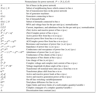
![Figure 2.2: The classical IEEE-39 bus transmission system [1, 2] ( c⃝1979 IEEE). The im-proved figure ( c⃝2015 IEEE) is copied from the IEEE-PES technical report PES-TR18 (Figure4.4) [3], which was first appeared from the 39 bus system MATLAB report [4].](https://thumb-us.123doks.com/thumbv2/123dok_us/8205030.261920/29.595.127.507.161.654/figure-classical-transmission-gure-technical-figure-appeared-matlab.webp)
![Figure 2.5: Schematic diagram of a synchronous generator from P. Kundur, Power SystemStability and Control [5] ( c⃝McGraw-Hill Education).](https://thumb-us.123doks.com/thumbv2/123dok_us/8205030.261920/45.595.190.458.116.307/figure-schematic-diagram-synchronous-generator-systemstability-control-education.webp)