E Health System Based on Statistical Equation Modeling

International Journal of Innovative Technology and Exploring Engineering (IJITEE) ISSN: 2278-3075,Volume-8 Issue-12, October, 2019

E-Health System Based on Statistical Equation

Modeling

Amandeep Kaur, Anuj Kumar Gupta

Abstract: In this research work, a design has been proposed for the Health Monitoring system that works with statistical equation models. The key advantage of this method is that it can work with different number of health parameters to through light on the health status of a person. The selection of the variables that will form the health monitoring model was done on the basis of three (Pearson, Kendall,spearman) correlation metrics. The root cause analysis based on OLS regression method confirms the mathematical relationship between the health indicators variables. It was found that visceral fat, as health indicator and as a dependent variable can act as function of seven other variables for knowing the health condition of a person. The validation of the model is done on the basis of multiple statistical tests.

Keywords: ehealth, mathematical modeling , casual analysis

I. INTRODUCTION

The penetration of electronic devices in developing countries [1] is quite high and deep [2] . But, the use of these electronic devices for improving the health quality [3] , [4] of the people at large has been damper . It has been reported that in most countries affordable health care is difficult to achieve and there is a need to use insurance instruments for cover up deficiencies of health care services and political will [5]. The contemporary literature shows that extending the geographic access of health [6], [3] care services is not only hard but difficult to realize due to unavailability of telecom /cellular infrastructure . Facilitation Services such as patient communication with the health care profession need to be improved. There is a need to improve data management and also to streamline the health care services with other industries for better and faster delivery of health care. At the same time , it can also be observed that there is a mounting interest in researchers in this context to change the way the health care is been monitored out in these countries [5],[6][7] .The use of radio, WI-FI , Bluetooth technologies are becoming more prevalent and there is a high hope that affordable health is now possible for many sections of society. The developing countries [1] are right now also witnessing an unprecedented increase in the number of users of sensor technologies. The smart mobile phones consist of many inbuilt sensors that can be used to track and monitor the fitness levels of the persons .But, for truly detecting the onset of diseases and complex health problems, medical grade medical sensors are required. And, other than these technological requirements the system need build in such a way that it removes the gaps between have and have-nots.

Revised Manuscript Received on October 10, 2019 * Correspondence Author

AmandeepKaur,Research Scholar ,Deptt of Computer Science

&Engg IKGPTU KAPURTHALA, PUNJAB. [email protected]

Anuj Kumar Gupta,Professor,Deptt of Computer Science &Engg,

CGC, LANDRAN, [email protected]

Hence, there is a need to analyses the various models been adopted by developing countries to tackle the problem of giving affordable health care [8]. The current literature shows that the use of statistical modeling is extensively used in monitoring health issues of the people. The statistical models form the basis for all the other emerging technologies such as machine learning [9]etc. It has also been found that the use of machine learning is typically useful only in those areas where the data volume is huge and technically it is defined as Big Data. However, for building health care models based on small datasets the preferred method is statistical modeling. In this research work statistical study of the health dataset has been explored for detecting the onset of health issues in person.

II. REVIEW

The process of mathematical modeling[10] helps to simplify the understanding of observed phenomenon. In medical domain[11] the observed phenomenon may be a health indicators or some kind of disease .The process leads to tractable description of the complex systems. In health sciences, mathematical modeling has been used in multiple ways to solve, simulate, investigate and understand the biological systems[12]. Accordingto[13] the probabilistic mathematical models are used in places where the observations are small in number or in cases , where the variables cannot be fully observed. The authors further say that, if the medical system can be understood with help of analogy, the mathematical system can be inspired from that process.For example, the amount of sugar stored in out body can be understood with help of a model called two compartment models[14], [15]. The focus of some authors is to make descriptive computational models. Such prototypes explain the real life conditions using tractable model of variables in terms of statistics tests[16]. The descriptive models are useful in community[17] and epidemiological studies. Typically,mean,mode, median, skewnessetc. are calculated and description of the phenomenon istranscribed.

In these areas of medical science heavily depends on the computer algorithms and automated computations. Models that involve time-series analysis[23] include physiological[24] reactions and variables such as blood pressure , pulse rate etc. need to be tracked and modeled for monitoring health issues.For deeper analysis models that help to understand the complex interactions are build using method called transfer functions . Such function basically tracks input output and the process in between. For example the transfer function for understanding the impact of sound wave impinging on human biological system. Electrocardiogram wave[25] analysis using mathematically modeling have been extensively by many authors[26]. In many cases, there is a need to do simulation [27]for understanding the health or medical issue . All simulation modeling begins with identification of active variables, latent variables and equations that map the real life conditions of the said problem. Examples such as simulation of genetic material transfer. Many authors have worked on simulation and modeling of epidemics[28],[29], [30],[31]and even studies on longevity.

In all these methods, simulation and models[32],[33] the underlying methods include use of mathematical equations, calculus and regression methods[34]. Many authors are using structural equation modeling (SEM)[35] to understand the relationship between the various health indicators and latent variables. In the process of finding and mapping mathematical relationship between the variables some authors are investigating the root cause of the health problem. The challenge , however , remains about selecting appropriate variables that can map the exact medical modality or phenomena[36]. Not, only this finding which set of variables can act as power predictors and which variable can explain the complete mathematical model remains a challenge. All the medical models discussed above rely on basic understanding of statistical process of modeling. The next section defines the scope of work based on the issues and challenges found in the current survey.

A. Scope of Work

Evidence from the industry, and after reading current challenges in the context of building health monitoring systems using mathematical modeling. Following scope of work has been formulated:

The scope of work will revolve around identifying variables that can be used for building sensor data based Health monitoring system. The model should be able to accurately find the values of factors that impact the dynamics of the heath of the person. Secondly, the selection of a group of variables that can be used for developing the Health monitoring system. And selection and validation of dependent and strong predictors for developing the Health monitoring system that can detect health issues from the stream of medical sensor data. Finally, the current work will include the evaluation of the statistical techniques that can predict the health issues accurately based on selected dependent and predictor(s) variables.

B. Assumed Design of Health Monitoring System

It is crystal clear from the review of the contemporized health monitoring systems that multiple types of technologies will together to make the system. The system includes the use of ultra-low powered devices that work with Bluetooth ,Wi-Fi, induction wireless, infrared wireless ,

ultra wide brand , Zee Bee, etc. The design Fig.1 shows the use of all such types‟ communication technologies.

Fig.1. Design of Health Monitoring System. The current review of the literature points out that interoperability technologies such as Restful API are making an exponential impact on design of decentralized systems such an eHealth Systems. The design, proposed here, also includes the use of Restful API to work with other industries such as insurance and fitness. Fig.1a layer wise approach in construction of the health monitoring system. The first layer will consist of the medical sensors that get connected to the sensor service interface (SSI). The sensor service interface (SSI) helps to connect to the core of the cloud as well as with the extended services that can be derived from the health systems such as fitness analysis (F.A) or insurance Analysis (I. A). The statistical functions for analysis of the health related issues are located in cloud core.

III. METHODOLOGY

International Journal of Innovative Technology and Exploring Engineering (IJITEE) ISSN: 2278-3075,Volume-8 Issue-12, October, 2019

Fig.2.WorkFlow of Research Work.

A. Data Characteristics

The data related to the health of a person was collected using an Omron Body composition machine and BP, sugar readings were also taken by apparatus from the same company. The data was collected over a period of three years (2016-2018) and the total data points collected were 2823. The data primarily consists of sixteen parameters. These parameters include Birth (BA) and body age (BDA), Height (H) ,Gender (G) , Weight (W) ,Body mass index (BMI), Body (BF) and visceral Fat (VF), Skeleton muscle (SM),Resting metabolism (RM) ,Waist (W), Blood pressure (BP) , Pulse rate (P) and Sugar readings (Sugar) before and after breakfast (Sugar PP) . All these sixteen parameters are indicators of life style problems and even inferences can be found that can be used to draw out grave health issues .

Table-I : Descriptive Analysis of the eHealth Dataset .

Table-Ishows that the data of parameter Birth age (BA) has an average of 41.46 and minimum body of the people is 17 years and maximum body age of the people is 89 years. The standard deviation is 14.1 , which means that there is age difference (spread ) of 14 years all over the data points of body age . Similarly, it can be observed that average Body Age (BDA) is 42.11 years. This value is not far from the mean value of birth age (41.46). Reflecting that, people are not aging faster as compared to their actual chronological age. But, the standard deviation of body age is more than birth age. This shows that there is a significant level of difference between birth age and body age. In this dataset, the difference is about 3%. The age weight of the people is

67.84 and average Body mass index (BMI) is 26.11. From, both these values, it is clear that on an average people are overweight (W) and are maintaining higher level of weights from the recommended weights. A similar trend can be seen in case of visceral fat (VF). The mean is coming close 12. Normally, the visceral fat should not be more than 6. The Skeleton muscle (SM) should normally be between 32.9 -35.7 for males and 20.9 to 29.9 for females. It can be observed that the minimum value is 19 and maximum values 59. From this it can be interfered that all types of cases healthy and unhealthy are there is the dataset, if Skeleton muscle (SM) is considered as criteria for declaring a person healthy/fit or not healthy. The Fasting Sugar (SF) value, if is greater than 140 shows bad state of health and if the value is between 120-140, it is borderline case of health issue. It may be a case pre-diabetic. Similar inferences can be drawn from the values of after meal Sugar reading test (SPP). The average pulse of the people here is 97.0 and minimum is 60. It is always desired that the pulse rate should be between 50 -60. Higher pulse rate shows that the heart of the person is working hard to circulate the blood all over the body. Table-I shows that some people have pulse rate as high as 150 showing that the dataset consists of cases that have very high heart beat rate. Similar, observation and understanding can be drawn from the values of Blood pressure (BpSys and Bpdia).

It is clear from the descriptive statistics that the dataset consist of many cases that reflect the current status of health of the people. For building a mathematical model of the detecting health issue from such dataset there is a need for understanding the behaviour and relationship between the variables. The next section investigates how the variables are behaving and how strong they are related to each other so that a mathematical model can be prepared. This is done with help of bivariate analysis using Pearson[37]Spearman and Kendall correlation formulas[38].

B. Health Variable Correlation Analysis

Table- II: Stable/Constant Co- variants Correlation Category wise.

C. Interpretation

The purpose of this analysis was also to find changing co- variants or constant variants. By definition changing variants are those pairs of variables that change when computed with the other method. In simple words, if a pair of variables has shown a strong relationship between them according to the Pearson method, the Kendall rank method and spearman methods should also show the same results. The analysis shows that all the methods are in concordance with each other. They all give similar output and show that there are no variable pairs that change their degree of association. Secondly, it was found that the pairs of variables need to be divided into six categories according to their average correlation values from the three methods. These categories are negative correlation, low correlation, medium correlation, high correlation, and very high correlation. Higher the average correlation value stronger is the association between them.

Since, this research work is a multi-year (2016-2018) study of health data for building mathematical model. A series of experiments were designed to find which variable causes changes in the other variable, so that a prediction model with discrepancies is constructed. The correlation test allowed us to identify group variables that are strongly associated and those pair of variable that exhibits no relationship (zero correlation) between them. Few pairs have negative correlation values, which mean as one variable changes the value of the other variable goes negative. From the table [II], it can observe that twelve pairs have negative correlation. The variables pairs that have zero correlation values will be useful for building regression based models because the prerequisite in regression is that variables should have property of being independent from each other‟s influence. In context of the problem undertaken here, there is need to investigate and find, which “dependent variable “ can map the relationship with other variables so that prediction can be made based on multiple combinations of health indicators. Hence, in the next section, causal analysis is done, so that a mathematical model can be built for predicting onset of a health issue.

IV. MATH

Mathematical Equation Modeling and Causal Analysis

A causal relationship establishes when one variable causes a change in another variable. These types of relationships are investigated by experimental research in order to determine if changes in one variable actually result in changes in another variable. For causal analysis, the process of experimentation establishes the case for using empirical results in real life. It established the fact that variable „x‟ is the root cause for changes in behaviour of the other variable „y‟. Hence, in this section a Multiple Dependent Variable Analysis (MDVA) is done. It will be used to model a pool of variables that vary together out of all the health variables and find which variable(s) can act as dependent variable best. This will be done so that numerically stable prediction model can be built and it confirms to the health quality dynamics. The tasks will include the use multiple regression tests (OLS regression method). And other statistical tests such R2, MSE that evaluate the quality of results it creates between the dependent variables and predictors for building equation based model. At the end of this section, the causal analysis will be presented with help of fish bone diagram. The reason of conducting a multivariate regression is to find which variable(s) can be used as a predictor of the dependent variable. The problem can be understood as “inverse problem”. An inverse problem is by “ a problem “ in which there is a large volume of samples of the variables but do not know how these variables interplay with each other. In the context of the problem undertaken here, there is a need to identify “dependent variables “as wells the best predictors for building the mathematical model for detecting onset of health issues.

The bivariate analysis based on correlation also clearly showed that in some pairs the dependent variable and predictor cannot strongly be explained. This was because the correlation values found by three methods confirmed that they low values of correlation. Hence, in this section, only those health variables be used for further analysis that impact each other. And, by proving null hypothesis,a causal analysis will be established or nullified. The design of experimentation (DoE) is shown in Table -III.

Table-III: Hypothesis for Finding Causal Relationship between the Variables.

Experiment No

Hypothesis

Dependent

Variable Best Predictors

1 Weight

Birth Age , Body Age , BMI , VF , BPSys ,

BPdia , Skeleton Muscle

2 Visceral Fat

Birth Age , Body Age , Weight , BMI , BPSys

, BPdia , Skeleton Muscle

3 Body Age

Birth Age , Weight , BMI , VF , BPSys ,

International Journal of Innovative Technology and Exploring Engineering (IJITEE) ISSN: 2278-3075,Volume-8 Issue-12, October, 2019

4

Blood Pressure Systolic

Birth Age , Body Age , Weight , BMI , VF ,

BPdia , Skeleton Muscle

5 Skeleton

Muscle

Birth Age , Body Age , Weight , BMI , VF ,

BPSys , BPdia ,

Experiment 1

Hypothesis: Is weight (WT) a function of all other variables that have strong association with other.

Fig.4.WT as Function of Other Variables InterpretationModel 1: The values of R-square in this case are 0.600, which means the model is a fair candidate model but not as good it should be. The standard errors in most cases are low. It may be attributed to the fact the coefficients of „VF and SM are negative even after the data values were centered close to mean. The values of p-values are good as they are zero in almost all cases, expect in BPdia (0.92). This further means that all variables are significant and important .The intercept is positive (9.93). The dataset has low level of skewness (shapes are not symmetrical) but overall distribution is has heavier tails. Due to which it seems that model could not acquire R-square value of 1. Therefore it cannot be said with good level of confidence that is no relationship between two groups (dependent and predictors of this model)

Experiment 2

Hypothesis: Is weight (VF) a function of all other variables that have strong association with other.

Fig.5.VF as Function of Other Variables

Interpretation of Model 2 :.The values of R-square in this case is 0.799 , which means the model is fairly good candidate model. The standard errors in most cases are close to zero. It may be attributed to the fact the coefficients of is negative. The values of p-values are good as they are zero. This means all variables are significant and important .The intercept is positive. The dataset has low level of skewness (shapes are not symmetrical) but overall distribution is has heavier tails. Due to which it seems that model could not acquire R-square value of 1.

Experiment 3

Hypothesis: Is Body Age (BA) a function of all other variables that have strong association with other.

Fig.6.BA as Function of Other Variables

Interpretation of Model 3: The p-values are zero of all the variables, clearly this means all the variables are significant and they should be included in the model 100%. The variable BMI and BPSys have negative correlation with the dependent variables (BA) but the other variables have positive correlation. The standard error is also low, except in case of BDA which means the difference between the actual and fitted values is somewhat within limits. But, the value of R square and Adj R-squared are 0.419. Hence, it is not a good fit. Hence, it seems that this model does not fairly explain the mathematical relationship between the BA and other variables. The F-statistic values also reconfirms that it is not a satisfactory model as it is high. A fair level of autocorrelation characteristic of the model is detected because the values of duban-watson test are around 1.233. Skewness is low. However, this model needs to discard.

Experiment 4

Fig.7.BPSys as Function of Other Variables. Interpretation of model 4: The p-values are zero , clearly this means all the variables are significant and they should be included in the model for sure. The variable BA and BPdia have small negative correlation with the dependent variables (BPSys ) but all other have positive correlation . This means the regression method had hard time finding good fit. And the R square value (0.744 ) shows it actually performed fair to find good fit and model needs to be rejected in case a better model is there. Clearly BPSys cannot act as function of all other variables if we compare this model with first model (VF) . The value of Durbin-Watson test is close to 1.2 which means data does not have good level of autocorrelation but a medium level.

Experiment 5

Hypothesis: Is Skeleton Muscle a function of all other variables that have strong association with other.

Fig. 8.Skeleton Muscle as Function of all Other Variables

Interpretation of model 5: This model shows R-square and Adj. R values close to 0.74. Clearly, this value is less than the VF model made in the first experiment of Durbin-Watson test is close to 1.2, which means the data does not have good level of autocorrelation but a medium level.

V.RESULTANDDISCUSSION A.Summary of all the models

It is clear that none of the model could acquire excellent level of “fitness “as none of the models have R-square value equal to 1. All models show that the selection of the variables is statistically significant. The values of t-test show that association between the dependent variable and independent variables cannot entirely be rejected. The dataset clearly has some degree of skewness and the distribution of skewness has heavy tails due to which in most cases the only two models could acquire (>0.74) value of R-square and one model (VF) attained Rsquare value of 0.799/. In most cases the AIC and BIC values are quite high (with negative and positive sign), which means good degree of information is embodied in the models.

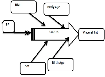
A. Causal Inference from all models

Based on this analysis, it can be concluded that the variable „VF‟ can act as function of other variables for predicting values. The variables BA, WT, BPSys, do have much effect on the values of other health indicators. The changes in the values of VisceralFat and do cause of change in values of BA, BDA, BMI, SM, BPSys and vice versa. This can be illustrated using Fish-bone Ishikawa diagram also.

Fig.9shows which parameters are impacting the VF variable. The value of VF can be calculated on the basis of all other seven parameters using following regression equation .Using the prescribed medical limits of visceral fat , the onset of the health issue can be detected using equation no 1 y = cax1 + cbx2 + ccx3 + cdx4 + cex5 + cfx6 + cgx7 + chx8 + cix9 +cjx10 + ckx11 + cl12 + z ……. (1)

where y is the dependent variable (VF ) and x1, x2 …..x12 are independent variables (WT,BMI, BPSys,BPDia,BA, BDA) related to y. The ca,cb, …….. clare coefficients computed by the OLS regression model inTable-IV.

Fig .9. Casual Analysis as Model 2. Table -IV: Coefficients and intercept of Model 2 Coefficients /

Regression Models

Coefficients z (Intercept)

OLS Model Experiment No 1

BA = 0.0038 BDA = 0.0911 BMI = 0.0128 WT = -0.0012 BPSys = 0.0039 BPDia = 0.0016 SM = 0.0011

International Journal of Innovative Technology and Exploring Engineering (IJITEE) ISSN: 2278-3075,Volume-8 Issue-12, October, 2019

y(VF ) = 0.0038*(BA) +0.0911*(BDA) - 0.0012*(WT) +0.0128*(BMI)–0.0039*(BPsys) –

0.0016*(BPdia)+0.0011*(SM) + 2.05e-14

VI. CONCLUSION

In this research, a mathematical model based on OLS regression method has been constructed after conducting multiple statistical tests. The selection of the variables for building the model was done on the basis of three methods of correlation and other inputs from descriptive analysis etc. It was found that eight variables have consistent high correlation values. This means that these variables had strong relationship with other. It made sense to consider only those variables that had influence each other. Therefore, a strategy was framed to find out, which variable can become a dependent variable and which variables can be powerful predictors of health status. Deeper investigation and by using five types of hypothesis it was found that Visceral Fat as health indicator is a powerful predictor of health of a person. It is fact, is established after conducting root cause analysis with other variables. It shows that increase in the values of other variables such a birth age, body age, basic metabolic rate , blood pressure will lead to increase in value of visceral fat value. From this model, information regarding the onset of health issue can also be extracted.

REFERENCES

1. S. Meghan, “Micro-Finance Health Insurance in Developing

Countries,” Whart. Res. Sch. Journal. Pap., vol. 62, 2010.

2. G. Sarin, “Developing Smart Cities using Internet of Things: An

Empirical Study Business Analytics View project Data Management View project Developing Smart Cities using Internet of Things: An Empirical Study,” no. March, 2016.

3. G. Pardeshi and V. Kakrani, “Mobile based Primary Health Care

System for Rural India,” Int. J. Nurs. Educ., vol. 3, no. 1, pp. 61–68,

2011.

4. Y. Balarajan, S. Selvaraj, and S. Subramanian, “Health care and

equity in India,” The Lancet. 2011.

5. K. S. Reddy, V. Patel, P. Jha, V. K. Paul, A. K. S. Kumar, and L. Dandona, “Towards achievement of universal health care in India by 2020: A call to action,” The Lancet. 2011.

6. A. Khandelwal, “E-health Governance Model and Strategy in India,”

J. Health Manag., vol. 8, no. 1, pp. 145–155, 2006.

7. M. Chokshi et al., “Health systems in India,” Journal of Perinatology.

2016.

8. B. D. Sommers, C. L. McMurtry, R. J. Blendon, J. M. Benson, and J.

M. Sayde, “Beyond Health Insurance: Remaining Disparities in US

Health Care in the Post-ACA Era,” Milbank Q., vol. 95, no. 1, pp. 43–

69, 2017.

9. S. Bhugra, N. Agarwal, S. Yadav, S. Banerjee, S. Chaudhury, and B.

Lall, “Extraction of Phenotypic Traits for Drought Stress Study Using

Hyperspectral Images,” in Lecture Notes in Computer Science

(including subseries Lecture Notes in Artificial Intelligence and Lecture Notes in Bioinformatics), 2017, vol. 10597 LNCS, pp. 608– 614.

10. H. E. A. Tinsley and S. D. Brown, “Multivariate Statistics and

Mathematical Modeling,” in Handbook of Applied Multivariate

Statistics and Mathematical Modeling, 2000.

11. B. L. Verma, S. K. Ray, and R. N. Srivastava, “Mathematical models

and their applications in medicine and health,” Heal. Popul. Perspect.

Issues, 1981.

12. Medical Applications of Controlled Release. 2019.

13. G. Baio and A. P. Dawid, “Probabilistic sensitivity analysis in health

economics,” Stat. Methods Med. Res., 2015.

14. J. Feng and G. Li, “Behaviour of two-compartment models,”

Neurocomputing, 2001.

15. E. Panagiotaki et al., “Two-compartment models of the diffusion MR

signal in brain white matter,” in Lecture Notes in Computer Science

(including subseries Lecture Notes in Artificial Intelligence and Lecture Notes in Bioinformatics), 2009.

16. A. P. Grieve, “Medical Statistics,” in The Textbook of Pharmaceutical

Medicine, 2013.

17. L. Star and S. M. Moghadas, “The Role of Mathematical Modelling in

Public Health Planning and Decision Making,” Purple Pap. Natl.

Collab. Cent. Infect. Dis., 2010.

18. J. Stausberg and M. Person, “A process model of diagnostic reasoning

in medicine,” Int. J. Med. Inform., 1999.

19. H. Valizadegan, Q. Nguyen, and M. Hauskrecht, “Learning medical

diagnosis models from multiple experts.,” AMIA Annu. Symp. Proc.,

2012.

20. M. Faraji et al., “Mathematical models of lignin biosynthesis Mike

Himmel,” Biotechnol. Biofuels, 2018.

21. J.-M. Scherrman, “Mathematical Modeling of Pharmacokinetic

Data.,” J. Pharm. Sci., 1995.

22. J. M. Anderson and L. S. Olanoff, “Pharmacokinetic Modeling and

Bioavailability,” in Medical Applications of Controlled Release,

2019.

23. D. Hand and M. Crowder, Practical longitudinal data analysis. 2017.

24. J. T. Ottesen, M. S. Olufsen, and J. K. Larsen, Applied Mathematical

Models in Human Physiology. 2004.

25. A. H. Khandoker and M. Palaniswami, “Modeling respiratory

movement signals during central and obstructive sleep apnea events

using electrocardiogram,” Ann. Biomed. Eng., 2011.

26. S. Ladavich and B. Ghoraani, “Rate-independent detection of atrial

fibrillation by statistical modeling of atrial activity,” Biomed. Signal Process. Control, 2015.

27. K. Cardona, J. F. Gómez, J. Saiz, W. Giles, and B. Trenor, “The effect of low potassium in Brugrada syndrome: A simulation study,” in Computing in Cardiology, 2014.

28. J. P. Chretien, S. Riley, and D. B. George, “Mathematical modeling of

the West Africa ebola epidemic,” Elife, 2015.

29. V. Colizza, A. Barrat, M. Barthélemy, and A. Vespignani, “The

modeling of global epidemics: Stochastic dynamics and

predictability,” Bull. Math. Biol., 2006.

30. E. T. Lofgren et al., “Opinion: Mathematical models: a key tool for

outbreak response,” Proceedings of the National Academy of Sciences

of the United States of America. 2014.

31. B. Tesla et al., “Temperature drives Zika virus transmission:

Evidence from empirical and mathematical models,” Proc. R. Soc. B

Biol. Sci., 2018.

32. J. A. Sokolowski and C. M. Banks, Modeling and Simulation in the Medical and Health Sciences. 2011.

33. S. I. Ringleb, “Physical Modeling,” in Modeling and Simulation in the

Medical and Health Sciences, 2011.

34. K. Bredies and D. Lorenz, “Mathematical preliminaries,” in Applied

and Numerical Harmonic Analysis, 2018.

35. T. N. Beran and C. Violato, “Structural equation modeling in medical

research: A primer,” BMC Res. Notes, 2010.

36. M. Ferdjallah and G. Kim, “Modeling the Human System,” in

Modeling and Simulation in the Medical and Health Sciences, 2011.

37. U. Bristol, “Data Analysis - Pearson‟s Correlation Coefficient,”

University of the West of England, 2018. .

38. James Lani, “Correlation (Pearson, Kendall, Spearman),” Statistics

Solutions, 2010.

AUTHORSPROFILE

Amandeep Kaur,has completed her Bachelor and Masters in Computer Science & Engg.She is a research scholar at IKGPTUKAPURTHALA,PUNJAB.She is working as Assistant Professor in CSE Department at BHSBIET Lehragaga, PUNJAB.She has teaching experience of thirteen years.Her area of interests are artificial intelligence, cloud computing and data mining. She has presented and published papers in National & International conferences and journals.