Manifolds
.
White Rose Research Online URL for this paper:
http://eprints.whiterose.ac.uk/129178/
Version: Accepted Version
Article:
Jiang, B, Li, Z, Chen, H et al. (1 more author) (2018) Latent Topic Text Representation
Learning on Statistical Manifolds. IEEE Transactions on Neural Networks and Learning
Systems, 29 (11). pp. 5643-5654. ISSN 2162-237X
https://doi.org/10.1109/TNNLS.2018.2808332
© 2018 IEEE. Personal use of this material is permitted. Permission from IEEE must be
obtained for all other uses, in any current or future media, including reprinting/republishing
this material for advertising or promotional purposes, creating new collective works, for
resale or redistribution to servers or lists, or reuse of any copyrighted component of this
work in other works.
[email protected] https://eprints.whiterose.ac.uk/
Reuse
Items deposited in White Rose Research Online are protected by copyright, with all rights reserved unless indicated otherwise. They may be downloaded and/or printed for private study, or other acts as permitted by national copyright laws. The publisher or other rights holders may allow further reproduction and re-use of the full text version. This is indicated by the licence information on the White Rose Research Online record for the item.
Takedown
If you consider content in White Rose Research Online to be in breach of UK law, please notify us by
Latent Topic Text Representation Learning on
Statistical Manifolds
Bingbing Jiang, Zhengyu Li, Huanhuan Chen,
Senior Member, IEEE
, and Anthony G. Cohn
Abstract—The explosive growth of text data requires effective methods to represent and classify these texts. Many text learn-ing methods have been proposed, like statistics-based methods, semantic similarity methods and deep learning methods. The statistics-based methods focus on comparing the sub-structure of text, which ignores the semantic similarity between different words. Semantic similarity methods learn a text representation by training word embedding and representing text as the average vector of all words. However, these methods cannot capture the topic diversity of words and texts clearly. Recently, deep learning methods such as CNNs and RNNs have been studied. However, the vanishing gradient problem and time complexity for parameter selection limit their applications. In this paper, we propose a novel and efficient text learning framework,
named Latent Topic Text Representation Learning (LTTR). Our
method aims to provide an effective text representation and text measurement with latent topics. With the assumption that words on the same topic follow a Gaussian distribution, texts are represented as a mixture of topics, i.e., a Gaussian mixture model. Our framework is able to effectively measure text distance to per-form text categorization tasks by leveraging statistical manifolds. Experimental results on text representation and classification, and topic coherence demonstrate the effectiveness of the proposed method.
Index Terms—Text Representation, Text Classification, Dis-tance Metric, Statistical Manifold, Gaussian Mixture Model.
I. INTRODUCTION
The problem of text categorization plays an important role in information retrieval, data mining, sentiment analysis, etc. Existing text classification methods can be divided into three categories: statistics-based methods, semantic similarity methods, and deep learning methods. Statistics-based methods, the traditional methods for text learning, include string kernels [1], term frequency-inverse document frequency (TF-IDF) [2] and naive Bayesian [3]. A string kernel [1] is a well-known kernel method for text classification, which focuses on similar subsequences that appear among multiple texts. The TF-IDF method organizes text into a vector space, which is usually based on a bag-of-words (BOW) model. Both approaches conform to the hypothesis that similar texts should have many
Bingbing Jiang, and Huanhuan Chen are with School of Computer Sci-ence and Technology, University of SciSci-ence and Technology of China (USTC), Hefei, Anhui 230027, China (e-mails: [email protected], [email protected]).
Zhengyu Li is with Advertisement Research for Sponsored search group in Sogou Inc, Beijing 100084, China (e-mail:[email protected]).
Anthony G. Cohn is with School of Computing, University of Leeds, Leeds, UK (e-mail: [email protected]).
This work was supported in part by the National Key Research and Development Program of China under Grant 2016YFB1000905, and the National Natural Science Foundation of China under Grants 91546116 and 91746209. Huanhuan Chen is the corresponding author.
words in common, but ignore the semantics of texts [4]. For instance, although the two sentences, ‘Obama invites the champion team to the White House’and‘The 44th President has dinner with the winning players in his home’, have no word in common, they convey almost the same semantic information.
Recently, a number of efforts have been made to learn a text representation based on semantic information. In [5], Mikolovet al. proposed the word2vec model, which is based on a distributional hypothesis and implemented by neural network language models. Le and Mikolov [6] proposed paragraph vector models, which incorporate paragraph matrix information to the input layer of continuous bag-of-words (CBOW) and Skip-gram models. A widely adopted semantic model is to build a text vector by simply averaging all word embeddings in this text. A word embedding is a mapping from words to vectors of real numbers, whose relative similarities correlate with semantic similarity [7]. Topic models are also effective semantic similarity methods for text learning [8]. Topic models, such as probabilistic latent semantic analysis (PLSA) [9], latent Dirichlet allocation (LDA) [10] and Gaus-sian LDA [11], [12], aim to capture the distribution of topics in the text. LDA groups similar words into similar topics and represents documents over these topics. The underlying idea behind LDA as a probabilistic language modeling method is that a topic is a distribution of words and a text is a distribution of topics. LDA assumes the distribution of topics in texts and words in topics both follow Dirichlet distributions. By contrast, Gaussian LDA assumes words in topics follow Gaussian distributions. However, these methods fail to measure the topic diversity of words and texts clearly. Although Liuet al. [7] proposed Topical Word Embeddings (TWE), in which each word has different embeddings in different topics, it only considers the topic diversity of words.
In the area of deep learning, the combination of the pre-trained word embedding and neural networks has also attracted muchs attention in recent years. Examples are recursive neural networks (RecursiveNNs) [13], [14], recurrent neural networks (RecurrentNN) [15], [16] and convolutional neural networks (CNNs) [17]. However, these neural network methods have some limitations. For example, a RecursiveNN discovers the semantics of a text by constructing a textual tree (e.g., RNTN [18]), which has at least a computational complexity of at least
O(n2), where n denotes the length of the text). Moreover,
Wikipedia corpus
word2vec
Word vector set
EM algorithm
Topic distributions represented by GMM
Specific text input
The probability distributions of specific texts
Text Representation of LTTR
Statistical manifold learning
The text representation on statistical manifold The distance
between text probability distributions
Text Distance Measurement of LTTR Distance
based classifiers (SVM, or KNN, etc.)
(1)
(2)
[image:3.612.140.473.55.238.2](3) (4)
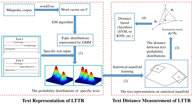
Fig. 1. An illustration of our method: (1) Given a specific text, a Gaussian mixture model is used to represent text as a probability distributionp(w|textt, θt). (2) Each text probability distribution is mapped as a point on a statistical manifold. (3) Following the framework of statistical manifolds, probability distributions are mapped into a parameter model space. (4) Learning text distance and applying it to distance-based classifiers to classify texts.
words. A RecurrentNN is a biased model and suffers from the vanishing gradient problem, which means that later words have greater impact than earlier ones. However, in practice, the key information may be distributed anywhere in a text rather than at the end. CNNs use a convolutional kernel, such as a sliding window with a pooling layer, to tackle the bias problem. However, there is a tension between performance and computational time: if a relatively small size of the sliding window is selected, the training will be accelerated but some critical information of a text may be missed, which is not good for the effective representation of a text, whereas a large sliding window size will enlarge the parametric space, which dramatically increases the training time.
Motivated by recent work, this paper presents a novel and efficient text learning framework to avoid the aforementioned issues. Our method aims to provide an effective text represen-tation based on word embedding and then learns a text distance measurement in the framework of a statistical manifold. The learning process of our framework is illustrated in Fig. 1. Firstly, word2vec [5] is employed to learn word vectors. Given the assumption that word vectors with the same topic follow a Gaussian distribution, then a Gaussian mixture model is used to describe the distributions of all words, in which each Gaus-sian represents a potential topic. In our method, a GausGaus-sian mixture model can represent a text with different topics. This model not only preserves the semantic information from word embedding but also builds a novel text representation from the perspective of text generation (i.e., the text is generated by several topics) [10]. Secondly, following the framework of the statistical manifold, each probability distribution can be viewed as a point on the statistical manifold. Based on information geometry [19], the distance between probability distributions is mapped into a metric in the parametric space of a statistical manifold, which can be applied to classify texts. The main contributions of this paper are summarized as follows:
1) We present a novel text learning framework. In this
framework, a text is represented as a mixture of topics, i.e., a Gaussian mixture model, which can effectively preserve the diversity of topic distribution.
2) By combining word embedding and topic models, our method can achieve better performance for text represen-tation and categorization, and topic coherence in com-parison with other state-of-the-art text learning methods. 3) From different measure theories, we discuss and analyse distance metrics between probability distributions. To ef-fectively quantify the distance between texts, we propose an efficient strategy based on the statistical manifold that produces a similar distance metric to that defined in functional space, confirming the validity of our method. The rest of this paper is organized as follows. Section II introduces the basic idea of word2vec and statistical man-ifold learning. Section III presents the proposed method in detail, including the text representation based on the Gaussian mixture model and distance metric learning in a statistical manifold. Section IV presents the experimental results and analysis. Finally, a conclusion is drawn in Section V.
II. BACKGROUND
A. word2vec
Word2vec1learns distributed word representations by using
neural network language models. The basic idea of word2vec is the distributional hypothesis [20], which states that words from the same context will have similar word representations. It constructs a log-linear classification network by a simple strategy for mapping words to real-number vectors [21]. Two models are proposed in word2vec: the CBOW model [5] and the Skip-gram model. The CBOW model is designed to predict the target word by context words, while the Skip-gram model is designed to predict context words from the target word.
For example, the CBOW model predicts each target word by context words in a sliding window. Given a tar-get word wt, the sliding window is a sequence Wt =
{wt−j, wt−j+1, . . . , wt, wt+1, . . . , wt+j}. The objective of CBOW is to maximize the log-likelihood probability:
L= X
wt∈corpus
logp(wt|context(wt)), (1)
wherecontext(wt) =Wt\ {wt}. Andp(wt|context(wt)can be defined as immediately below via softmax functions:
exp(v′wt
TP
wt∈context(wt)vwt)
P
w∈corpusexp(v ′ w
P
wt∈context(w)vwt)
, (2)
where vwt and v
′
wt denote the “input” and “output” vector
representations of the word wt.
Word embeddings trained by word2vec also have linguistic regularity [22]. The assumption is that words belonging to the same topic have similar word vectors and this is also the basic idea of text representation in our proposed method.
B. Manifold learning
Manifold learning assumes that low-dimensional data is of-ten embedded in a high-dimensional space [23]. The main goal of manifold learning is to recover the data’s low-dimensional manifold structure. Because of this, manifold learning has been widely used to reduce dimensionality for nonlinear structure data [24]–[30].
Theoretically, a Riemannian manifold (M, g)is a differen-tiable manifold M equipped with Riemannian metric g. At each point p∈M,gp is a positive-definite quadratic form on the tangent space of each pointp. Thus we obtain the definition of length, area, or volume on a Riemannian manifold. For example, if C : [a, b] → M is a continuously differentiable curve in the Riemannian manifoldM, and the parameterized equation isC(t), then the curve’s length is defined as:
L(C) = Z b
a
X
i,j gij
dxi dt
dxj dt
12
dt, (3)
where dxdti is the i-th component of a tangent vector at point
x= (x(1), . . . , x(D)). Moreover, with this definition of length,
the distance between two pointsx,y onM is defined as:
d(x, y) =inf{L(C)}, C∈C, (4)
where C is the set of continuously differentiable curves that
join x and y. Eq. (4) defines the distance between two points as the length of the shortest curve on the manifold. If the probability distributions associated with the points of a Riemannian manifold are replaced with statistical models, then a statistical manifold will be formed.
III. TEXT REPRESENTATION LEARNING WITH STATISTICAL MANIFOLDS
In this section, our method will be introduced in three parts. Firstly, a Gaussian mixture model is used to represent text as a probability distribution. Then, we discuss and analyze the distance metric between probability distributions, and then propose to measure text distance under the statistical manifold learning framework. Our approach is illustrated in Fig. 1.
A. Text representation based on Gaussian mixture model
Word2vec can learn word vectors for words from a large corpus by using the CBOW or the Skip-gram. Our method improves on such word embeddings to a text representation. It is based on the view that text is generated from a combination of topics. This idea is inspired by topic models [9], [10].
Firstly, each word is considered as a point in word space, and it distributes in the word space according to its potential topics. For example, ‘Illinois’ and ‘Chicago’, ‘stock’ and ‘tax’, are close in word space due to containing the same topic, which means that the words in the same topic have similar word vectors and might be relatively close in word space. Therefore, we assume that word vectors in the same topic follow a Gaussian distribution. Building on this assumption, a Gaussian mixture model is used to describe the distribution of all words. Given all word vectorsV ={w1, . . . , wN}, the mixture density is:
p(w) = K X
i=1
πiN(w|µi,Σi), (5)
where πi is the weight coefficient of each component, K is the number of topics. In our method, each component represents a potential topic but it is not required to know which topic each component expresses. N(w|µi,Σi) is a Gaussian distribution with mean µi and variance matrix Σi. The i-th topic is the most probable topic that wordwbelongs to, when
πiN(w|µi,Σi)is maximum among all Gaussian components. It can be used to label each word by its most likely topic. In our method, each word plays a different role in different topics, preserving the topic diversity from words and texts. The probability that the wordw belongs to thei-th topic is:
p(topici|w) =
πiN(w|µi,Σi) PK
i=1πiN(w|µi,Σi)
. (6)
We estimate the parameters µi,Σi andπi of the Gaussian mixture model using the Expectation-Maximization (EM) al-gorithm. The estimation process is presented as follows [31]: (1) Initialize the weight coefficients πi, means µi, and covariancesΣi (i= 1,2,· · · , K).
(2) E-step: Use current parameter values, evaluate the responsibilitiesγjithat thei-th Gaussian component takes for representing the j-th word vectorwj:
γji=
πiN(wj|µi,Σi)
PK
i=1πiN(wj|µi,Σi)
, i= 1,2,· · ·, K;j= 1,2,· · ·, N.
(3) M-step: Re-estimate the parameters using the current responsibilities:
πi= PN
j=1γji N ; µi=
PN j=1γjiwj PN
j=1γji
, i= 1,2,· · ·, K
Σi= PN
j=1γji(wj−µj)(wj−µj)T PN
j=1γji
(4) Evaluate the log likelihood with respect to the parame-ters:
lnp(V|µ,Σ, π) = N X
j=1
ln
K
X
i=1
πiN(wj|µi,Σi)
. (7)
Check for convergence of the parameterπi. If the convergence criterion is not satisfied, repeat steps (2) and (3).
Furthermore, a text can be viewed as a subspace of word space: words in a text are a recombination of all words according to the topics. Therefore, for a specific text textt in the text set T ={text1, . . . , textn}, it can be represented as:
p(w|textt, θt) = K X
i=1
θ(ti)N(w|µi,Σi), t= 1,2, . . . , n; (8)
where θt is a weight coefficient vector that reflects the proportion of different topics in the text. It can be ob-served that each Gaussian component is the same as Eq. (5), although the weight coefficient has changed due to the recombination of words. Each coefficient reflects the propor-tion of the corresponding component (or potential topic) in the text. According to Eq. (6), the contribution from word
w to topici is p(topici|w). Thus, the weight of topici in the text is P
w∈texttπiN(w|µi,Σi). To ensure the condition
PK i=1θ
(i)
t = 1, the weight coefficient of each Gaussian component can be calculated by:
θ(ti)= P
w∈texttπiN(w|µi,Σi)
PK i=1
P
w∈texttπiN(w|µi,Σi)
, i= 1,2, . . . , K. (9)
For example, if we use Eq. (8) to represent a paper about machine learning, the weight coefficient of the topic ‘biology’ may be very close to zero, while the topic ‘clustering’ may have a larger weight coefficient.
As stated above, we use a Gaussian mixture model as a probability density function to provide a representation of a text, which considers semantic information and the diversity of topic distribution between words. We now discuss how distances between Gaussian mixture models can be obtained.
B. Distance metric between probability distributions from different measure theories
In the previous subsection, each topic is represented as a Gaussian distribution, and thus texts are represented as proba-bility distributions, i.e., the Gaussian mixture models (GMMs) with the same Gaussian components. In order to classify texts effectively, a distance metric is needed to measure the distance between texts, i.e. how much they differ. In this subsection, we will discuss and analyze how to measure the distance between text probability distributions under different measure theories. 1) Jensen-Shannon divergence: In probability and infor-mation theories, the Jensen-Shannon (JS) divergence [32] provides a similarity of probability distributions. It is based on the Kullback-Leibler (KL) divergence [33] and provides a symmetric and smooth version of KL divergence. Given two
text probability distributionsP andQof a continuous random variablex, the JS divergence betweenP andQis defined as:
J(P||Q) = 1
2DKL(P||M) + 1
2DKL(Q||M), (10)
where M = 12(P +Q), and DKL(P||Q) denotes the KL divergence betweenP andQ.
For two Gaussian distributions, the KL divergence has a closed-formed expression. However, the KL divergence has no analytical solution for Gaussian mixture models. Although some techniques have been introduced to solve this problem, such as Monte Carlo sampling, unscented transformation [34], variational approximation and so on, these methods will be unstable with a relatively larger error when the dimension of the random variable x or the number of the Gaussian components in GMMs is large [35]. Thus, they are not suitable for measuring the distance between texts from the theoretical perspective.
2) Hellinger distance: In probability and statistics, the Hellinger distance is used to quantify the similarity between two probability distributions. The squared Hellinger distance between probability distributionsP andQis defined as:
H2(P, Q) = 1 2
Z p
f1(x)−
p
f2(x)
2
dx
= 1− Z
p
f1(x)f2(x)dx.
(11)
In our method, f1(x) = PKi=1θ (i)
1 N(x|µi,Σi), f2(x) =
PK i=1θ
(i)
2 N(x|µi,Σi)denote the densities of text probability distributions, making the Hellinger distance between texts hard to directly calculate from the theoretical perspective.
3) Wasserstein distance: Unlike the KL divergence, the Wasserstein metric not only measures the change of probability distribution but also incorporates the underlying geometry between them. Given two probability distributions P andQ, the 2-Wasserstein distance is defined as:
W2(P, Q) = infEPxy
kx−yk2 2
1/2
, (12)
wherexandy are the random variables ofP andQandPxy denotes their joint distribution. The Wasserstein metric is the minimum cost of moving the random variable from probability distributionP toQ, which describes the changing of weights in GMMs. However, Wasserstein metric is computationally expensive to calculate for high-dimensional random variables. 4) Lp space distance in functional space: In functional analysis, Lp space is often defined as a functional space. It provides the p-norm distance between two functions f1(x)
andf2(x). Letp= 1, then the1-norm distance is given by:
L1(f1(x), f2(x)) =
Z
||f1(x)−f2(x)||dx
= Z K
X
i=1
||θ(1i)−θ (i)
2 ||N(x|µi,Σi)dx
=||θ1−θ2||1,
(13)
often used since it is more smooth. Let p = 2, the 2-norm distance between f1(x)andf2(x)in functional space is:
L2(f1(x), f2(x)) =
Z
||f1(x)−f2(x)||2dx
1/2
= Z K X i=1 K X j=1
didjN(x|µi,Σi)N(x|µj,Σj)dx 1/2
= K X i=1 K X j=1
didjmij 1/2
=q(θ1−θ2)TM(θ1−θ2),
(14)
where di =θ(1i)−θ (i)
2 , mij ∼ N(µi|µj,Σi+ Σj)andM =
(mij)K×K. Compared withL1distance,L2 can preserve the
diversity or similarity among different Gaussian components. In Eq. (14), M can be regarded as a correlation information matrix of different Gaussian distributions. However, calculat-ing matrix M and text distance in Eq. (14) require O(K2d3)
and O(K2d2) computational complexity, respectively, which
will dramatically increase the running time for a large topic numberK or a high word vector dimensiond.
C. Text distance metrics with statistical manifold learning
In our method, texts are represented as Gaussian mixture models, and the space composed of these Gaussian mixture models can be viewed as a statistical manifold. A statistical manifold is a special case of a Riemannian manifold, whose elements are probability distributions. As stated in Section II, Eqs. (3) and (4) provide the distance metric between two points on a Riemannian manifold. However, on a statistical manifold, each point is a probability distribution, which means that the distance between probability distributions cannot be directly measured by using Eqs. (3) and (4).
In statistical manifold learning, probability distributions are usually mapped into a parameter space [36]. Considering S
as a family of probability distributions, andS ={p(x|λ)|λ= [λ(1), λ(2), . . . , λ(n)]}, in whichλis called a parametric space
and S is called a parametric model. In this paper, texts are represented as probability models (i.e., Gaussian mixture mod-els with same Gaussian components). Therefore, a Gaussian mixture model can be seen as a family of probability distribu-tions that distributes on a statistical manifold. When mapping the text probability distribution to a parametric model, the parametric model can be defined as the coordinates of the statistical manifold. In Eq. (8), the Gaussian mixture model can be defined as a function in functional space, each Gaussian component N(w|µi,Σi)can be viewed as a base function of the function space and the parametersθdenote the coordinates on a Riemannian manifold. Therefore the statistical manifold of the Gaussian mixture model is parameterized by θ = [θ1, . . . , θK]. The parametric model is S = {p(w|text, θ)}. According to information geometry, Riemannian geometry can be used to learn underlying information from a statistical model [19]. Therefore the parametric model can be embedded in a Riemannian manifold.
It should be noted that the space of a parametric model is a continuous and differentiable manifold. Moreover, according to the properties of a Gaussian mixture model,θ1+. . . , θK=
1. Hence the shape of the parametric manifold is a hyperplane of dimensionK−1. It is shown on the right-hand side of Fig. 1. Therefore, the geodesic curve in a hyperplane is a straight line, and the shortest curve that joins two pointsα andβ in the manifold is:
C(u) =α+ (β−α)u, u∈[0,1]. (15)
Thus, according to Eq. (3), the distance between αandβ is:
d(α, β) =L(C(u)) = Z 1
0
(X i,j
gij dC(u)
dui
dC(u)
duj )
1 2du = Z 1 0 (X i,j
gij((βi−αi)(βj−αj))
1 2du
=q(β−α)TG(β−α),
(16)
where the Riemannian metric gij measures the correlation between different dimensions andG= (gij)K×K is similar to M in Eq. (14). The Fisher information metric, which provides the similarity measurement, can be used to define the metric on the Riemannian manifold. It can be computed as [37]:
gij(θ) =
Z ∂ln p(x|θ)
∂θi
∂ln p(x|θ)
∂θj
p(x|θ)dx
=Ep(x|θ)
"
N(x|µi,Σi)N(x|µj,Σj) PK
i=1θiN(x|µi,Σi) #
,
(17)
where the expectation defines the similarity or overlap between topics i and j on the Riemannian manifold. From Eq. (17), we note that it is hard to directly calculate the closed-form expression for gij. In our method, we can sample according to the text probability distribution p(x|θ), then calculate the approximated values for gij. Asymptotically, however, the Fisher information metric is immaterial, and it may be ignored in practice [38], [39]. Often, the Kronecker delta function is used as a replacement i.e., G=I [39],
gij =δij =
1 i=j,
0 i6=j. (18)
Thus, substituting gij in Eq. (16) with Eq. (18), the distance betweenαandβ becomes:
d(α, β) = Z 1
0
(X i,j
δij((βi−αi)(βj−αj))
1 2du = Z 1 0 (X i
(βi−αi)2)
1
2du=kβ−αk2.
(19)
Eqs. (16) and (19) provide the distance metric between two texts with different measurements. It is worth pointing out that if we usemij to replace the value ofgij, the distance between αandβ becomes:
d(α, β) =L(C(u)) = Z 1
0
(X i,j
mij dC(u)
dui
dC(u)
duj )
1 2du = Z 1 0 (X i,j
mij((βi−αi)(βj−αj))
1 2du
=q(β−α)TM(β−α) =L
2(f1(x), f2(x)).
Eqs. (20) and (14) give the same results under different theoretical approaches. In fact, Eqs. (20) or (16) can preserve more diversity or similarity information among different topics than Eq. (19). However, if the dimension of word vectors and the number of the Gaussian components are large, the calculation of matrix M orGwill be very difficult and time-consuming. Thus, we use Eq. (19) to calculate the text distance in the experiments. The intuitive explanation is that a larger number of topics enable the topics to be fully separated and independent, and the overlaps between different topics are fewer, which means that each topic may have a more equal weight.
Algorithm 1 Measure latent topic text representation on statistical manifold
1: Input:Word embeddings V ={w1, . . . , wN} trained by word2vec, texts for trainingT ={text1, . . . , textn}.
2: Output: Distance matrixD between each pair of texts. 3: Given word embeddingsV, estimate the parametersµi,Σi,
andπi of Gaussian mixture model by the EM algorithm.
4: Calculate the topic labels of each word using Eq.(6) (word label list) based on the Gaussian mixture model.
5: foreachtextt(t= 1,2,· · ·, n) inT do
6: initialize parametric modelθt= (0, . . . ,0)for textt.
7: foreach wordwintexttdo
8: θt(i)=θ(ti)+πiN(w|µi,Σi),i= 1,2,· · · , K.
9: end for
10: Normalizing weight coefficientθt=θt/Piθ
(i)
t .
11: end for
12: foreach pair oftexti,textj∈T (i, j= 1,2,· · ·, n),do
13: D(i, j) =d(θi, θj), andd(θi, θj)is defined in Eq. (19).
14: end for 15: returnD.
In our representation of text, the semantic information from word embeddings is preserved in each Gaussian component. Moreover, the proportion of different topics in the text can be expressed by the weight coefficient vector θt. The algorithm of Latent Topic Text Representation (LTTR) is summarized in Algorithm 1. First of all, the parameters of the Gaussian mixture model are estimated by the EM algorithm, then the word label list is constructed by the Gaussian mixture model. For each text, we initialize the parametric model θtas a zero vector and then calculate the weight coefficient vector θt by using Eq. (9). After that, θt is standardized to ensure the condition θ(1)t +θ
(2)
t +. . .+θ
(K)
t = 1. Finally, the distance between texts is calculated using Eq. (19). The most time-consuming part of the proposed method is to construct all word label lists using a Gaussian mixture model. After that, the computation complexity of the text representation is O(W), in which W is the total number of words in the text.
In this paper, we propose a novel and efficient text learning framework, which aims to provide an effective text representa-tion and text measurement with latent topics. Therefore, there are two learning objectives in our method. One is to develop an efficient text representation model that can preserve the seman-tic information of texts and the diversity of topic distributions. The other is to effectively measure the distance between
text probability distributions that can be directly applied for text categorization. The learning process of our framework is illustrated in Fig. 1. At the text representation stage, the parameters to be learned includeπi,µi, andΣiin the Gaussian mixture model, and the weightsθtthat reflect the proportions of the topic in a specific text, textt. The parameters πi, µi, and Σi are estimated by using EM algorithm to maximize the log-likelihood function with respect to them in Eq. (7) (i.e., the objective function), and θt is calculated by Eq. (8). In our method, word vectors belonging to the same topic are assumed to follow a Gaussian distribution, then texts are represented as probability distributions, i.e., Gaussian mixture models. Therefore, in the text distance measurement stage, the learning objective is how to effectively quantify the distance between text probability distributions. The measure of distance between probability distributions remains an open question. In Section III-B, we have discussed and analyzed the distance measure between text probability distributions from different measure theories. In Section III-C, we introduce the statistical manifold, then convert the measurement of text probability distributions on the statistical manifold to the parametric space. Therefore, the distance between text probability distributions is calculated, which can be directly applied to the distance-based classifiers to perform text categorization.
IV. EXPERIMENTALSTUDIES
A. Experimental Datasets
In this paper, the datasets in the experiments are chosen from three news corpora. Each dataset contains news of different classes.
• BBC News2: The BBC dataset is built on BBC News,
provided as benchmarks for machine learning research. The dataset consists of 2285 documents from the BBC news website corresponding to stories in five topical areas. The information is shown in Table I.
TABLE I
BBCNEWS DATASET
Class train docs test docs Total docs
business 340 170 510
entertainment 258 128 386
politics 278 139 417
sport 341 170 511
technology 268 133 401
Total 1485 740 2285
• Reuters 215783: This dataset appeared on the Reuters
newswire and was manually classified by Reuters person-nel. There are two versions of the dataset R8 and R52, the latter has 52 topics but the distribution is very skewed, hence here we use R8 with 8 topics. The distribution of documents per class is shown in Table II.
• 20 newsgroups3: This dataset is a collection of approx-imately 20,000 news items, and it contains 11293 items for training and 7528 items for testing. The distributions of training and test data are shown in Table III.
2http://mlg.ucd.ie/datasets/bbc.html
TABLE II
REUTERS21578 R8DATASET
Class train docs test docs Total docs
acq 1596 696 2292
crude 253 121 374
earn 2840 1083 3923
grain 41 10 51
interest 190 81 271
money-fx 206 87 293
ship 108 36 144
trade 251 75 326
Total 5485 2189 7674
TABLE III
20NEWSGROUPS DATASET
Class train docs test docs Total docs
alt 480 319 799
computer 2917 1952 4869
misc 585 390 975
rec 2389 1589 3978
science 2373 1579 3952
society 598 398 996
talk 1951 1301 3252
Total 11293 7528 18821
B. Experimental Settings and Word embedding training
In our method, the CBOW model is used to train word embeddings. According to the analysis in [40], in order to reduce the calculation time and keep the high-level expression of word vectors, we analyze the parametric sensitivity with the dimensionality of vector and the size of the sliding window. In training, a hierarchical softmax strategy is adopted to speed it up. A word vector list is trained with theWikipediacorpus, which contains millions of words and sentences. This corpus is also used in other methods which needs a corpus for training. Table IV presents the accuracy of LTTR with KNN on the test documents of Reuters by using two kinds of word2vec models (i.e., CBOW and Skip-gram) with different vector lengths and window sizes.
TABLE IV
ACCURACY(%)ONREUTERS DATASET WITHK=300INLTTRWITH
k-NNCLASSIFIER
vector length window size
accuracy with different word2vec models
CBOW Skip-gram
2 84.52 82.21
50 5 85.13 82.44
10 84.52 82.44
2 90.32 88.46
100 5 91.17 90.87
10 91.03 89.73
2 92.04 94.20
150 5 94.38 94.17
10 93.34 92.96
2 93.80 94.17
200 5 94.06 94.19
10 94.04 92.17
2 91.96 93.77
300 5 92.43 92.08
10 93.12 92.80
In Table IV, the 3rd and 4th columns denote the accuracies of adopting the CBOW model and Skip-gram model, respec-tively. The results on the parametric sensitivity of word2vec
models shown in the table provide an empirical basis for choosing the parameter of our experiments. For example, we notice that when word vector length=150 and window size=5, LTTR using the word vectors trained by CBOW model achieve the best performance. For convenience, this setting is used for the subsequent experiments. Better performance could be achieved by evaluating possible parameter settings with more finely grained chosen values, which would of course require further training time.
In the experiments, stop words are removed from experi-mental datasets to avoid the influence of irrelevant words. As stated in Section III-A, a Gaussian mixture model is used to describe the distribution of all words. The number of Gaussian components in GMMs (i.e., the number of topicsK) is chosen to optimize the experimental results, and the details of the sensitivity analysis of the parameterK are shown in Fig. 5.
C. The Results and Analysis of Text Classification
1) Comparison with related work: We evaluate our method for text classification tasks by using the k-NN and SVM classifiers. The distance between texts is defined as Eq. (19) in Section III-C, which can be used for k-NN and SVM to classify text. In the following, we compare our method with other text learning methods:
• TF-IDF [2]. This method is a modified bag-of-words model. The element of the vector is the document fre-quency of the corresponding word.
• Topical Word Embeddings (TWE) [7]. TWE allows each
word to have different embeddings under different topics by utilizing latent topic model. The text embeddings generated by word embeddings are used as text features.
• word2vec: In this paper, we use the average vector of all
the words in a text to represent a text.
• Distributed Memory Model of Paragraph Vectors (PV-DM) [6], which incorporates paragraph matrix informa-tion to the input layer of CBOW. In this model, every paragraph is mapped to a unique vector, and every word is also mapped to a unique vector. The paragraph acts as a memory that remembers what is missing from the current context or the topic of the paragraph.
• Latent Dirichlet Allocation (LDA) [10]. LDA is a method which belongs to topic model methods [41]. It assumes that each text is a mixture of topics and each word has a topic label. In this method, the text is compressed into a vector. Each component of the vector is the probability of topics included in the text. Therefore, the topic information is used as text features for LDA.
• Gaussian Latent Dirichlet Allocation (Gaussian LDA)
[11]. This model is developed based on the framework of LDA, which replaces the parameterizations of topics in LDA as the multivariate Gaussian distributions on the embedding space. This model can infer different topics relative to standard LDA.
TABLE V
TEST RESULTS(%)ON EACH DATASET
Method TF-IDF TWE word2vec PV-DM LDA Gaussian LDA CNN LTTR
Classifier SVM K-NN SVM K-NN SVM K-NN SVM K-NN SVM K-NN SVM - K-NN SVM
BBC news 78.11 91.99 92.32 91.49 91.99 91.74 92.43 93.65 93.09 93.46 94.12 94.83 94.75 95.68
Reuters 71.38 91.52 91.67 93.24 93.07 93.56 93.32 93.14 93.65 93.22 93.78 94.21 94.38 93.55
20newgroups 46.59 69.67 68.87 72.86 70.56 72.52 71.01 69.85 69.77 72.21 72.43 72.95 74.63 73.22
business enertainment politics sport technology 0.7
0.75 0.8 0.85 0.9 0.95 1
LTTR word2vec LDA
(a) Recall rates on BBC news dataset
business entertainment politics sport technology 0.8
0.85 0.9 0.95 1
LTTR word2vec LDA
[image:9.612.346.541.280.368.2](b) Precision rates on the BBC news dataset
Fig. 2. The recall and precision rates of different methods on the BBC news dataset
acq crude earn grain interest money ship trade 0.4
0.5 0.6 0.7 0.8 0.9 1
LTTR word2vec LDA
(a) Recall rates on R8 dataset
acq crude earn grain interest money ship trade 0.6
0.7 0.8 0.9 1
LTTR word2vec LDA
[image:9.612.77.275.281.379.2](b) Precision rates on the R8 dataset
Fig. 3. The recall and precision rates of different methods on the R8 dataset
alt computer misc rec science society talk 0.2
0.3 0.4 0.5 0.6 0.7 0.8 0.9
LTTR word2vec LDA
(a) Recall rates on 20newsgroup dataset
alt computer misc rec science society talk 0.4
0.5 0.6 0.7 0.8 0.9
LTTR word2vec LDA
[image:9.612.76.273.415.513.2](b) Precision rates on the 20newsgroup dataset
Fig. 4. The recall and precision rates of different methods on the 20newsgroup dataset
The experimental results of the proposed method and other state-of-the-art methods on text classification tasks are pre-sented in Table V. The results are classification accuracy of each method with different classifiers on the test sets, and the best performance on each data set is highlighted. From Table V, we observe that PV-DM obtains comparable performance with word2vec, and Gaussian LDA achieves slightly better performance than LDA, but they are still inferior to our method. Although CNN obtains comparable performance with our method, CNN as a deep learning method, has a limitation that it is expensive to tune parameters, as discussed in Section I. In LTTR, we assume that words on the same topic follow a Gaussian distribution, and then texts are represented as a Gaussian mixture model, whose parameters are learned with the help of the EM algorithm. The complexity of text modeling isO(W), and the complexity for calculating the text distance
isO(K2), whereW is the number of words in the text, andK
is the number of topics. Therefore, while the CNN achieves comparable accuracy, the proposed LTTR is more efficient. Therefore, the results show the effectiveness of the proposed method on text classification tasks in comparison with other methods.
TABLE VI
15WORDS WHICH HAVE A HIGHER PROBABILITY DENSITY IN EACH TOPIC ORGAUSSIAN DISTRIBUTION
topics animal economy education internet language politic science social sports
words
species supply school network english members research society football
animals investment students access speaking council study freedom professional
fish prices degree connection ungrammatical parliament scientific moral teams
birds budget classes mail dialects elected institute intellectual competition
mammals inflation teaching servers grammar committee engineering liberty hockey
insects debt universities sharing vocabulary executive learning collective olympic
endangered benefits colleges hubs literacy senate psychology individualism basketball
whales fiscal graduate wap lexicon legislative geology motivation cricket
zoo taxation junior wifi phonetics ministers psychology morally contest
hunters oversupply courses timestamping arabic representatives humanities argues championships
lizards industrializing lessons broadband anglophones cabinet biomedical unequal tournament
feral overvalued exam lan esperanto presidents linguistics persuasion leagues
predator surplus majors bbs fluent ombudsman astronomy democracy arena
snakes policies coursework clients lingua house mineralogy servile rankings
cetaceans demand pedagogy distributed multilingual meeting informatics unjust spectator
100 200 300 400 500 600
0.65 0.7 0.75 0.8 0.85 0.9 0.95
Accuracy
K
[image:10.612.59.322.78.380.2]BBCnews Reuters 20ng
Fig. 5. Accuracy changes (k-NN classifier) on all datasets with differentK
in Gaussian mixture models
LTTR with KNN is definitely biased towards achieving higher accuracy on Reuters due to more suitable parameter settings. Another possible reason is the distribution of data sets. For the balanced text data, like BBC news, SVM can easily find an optimal decision hyperplane and produces a higher accuracy than KNN [42]. However, it might be difficult for an SVM to find the optimal hyperplane on multi-class imbalanced text data, like Reuters and 20newsgroups. In fact, this problem is a worth-studying direction in the future.
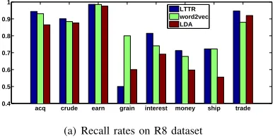
From Table II-III, we know that the Reuters R8 and 20 newsgroup datasets are unbalanced. In order to better evaluate the effectiveness of our method for text classification, two common evaluation metrics, the precision and recall rates, are adopted. The precision and recall rates of different methods on each dataset are analyzed. As typical models, LDA and word2vec are selected to compare with our method. The word vector length is set to 150 in word2vec and the number of topics is set to 300 in LDA and LTTR. The results are shown in Figs. 2-4. From Table I, we know the BBC news is a balanced dataset. In Fig. 2, we observe that our method obtains promising performance in terms of recall and precision rates on each class of BBC news dataset. It can be observed that the precision and recall rates in Figs. 3 and 4 reflect the imbalance intuitively. From Table II, we know that the size of text that belongs to ‘gain’ is few, and the text length is shorter. Fig 3 shows that our method is not better than word2vec in recall
rate on the class ‘gain’. The result may demonstrate that the words play a more important role than the topic in short text classification. In Fig. 4, we note that the recall rate of class ‘society’ is high but the precision is pretty low for all methods, which demonstrates that class ’society’ overlaps with other classes. The classifiers might categorize text belonging to other classes into the class ‘society’.
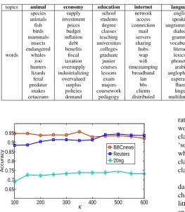
We also analyze the parametric sensitivity of K on each dataset. The result is shown in Fig. 5. It can be observed that changing the parameterKin the Gaussian mixture models has little effect on the performance of LTTR. In view of Table IV and Fig. 5, it also shows the stability and robustness of our proposed method with respect to the number of topicsK.
D. Experimental Results and Analysis for Text Representation and Diversity Preservation of Topic Distribution
To evaluate the ability to describe the word vector distri-bution while using the Gaussian Mixture Model, we select some representative topics for visualization. The results are shown in Table VI. Each column represents a topic, 15 words with a higher probability density in each topic or Gaussian distribution are presented. It can be observed that the matching of words and topics is good in our method.
In our method, the diversity of topic distributions is also considered. Four words {class, power, doctor, right} are selected as targets, and they all may belong to at least two possible topics.
The probability that word w belongs to the i-th topic is calculated by Eq. (6), and then the topics with a higher probability are selected. The results are given in Table VII, which shows the diversity of topic distributions is effectively preserved from words. For example, the word‘doctor’belongs to two topics which have a higher probability than that of others. We list some words which have a higher probability density in the selected topic from Table VI. It shows that the most probable topic that word‘doctor’belongs to is medical science, the second is academic degree.
TABLE VII
MIXTURE DISTRIBUTIONS OF TOPICS ON TARGET WORDS
target word
mixture topics
words with higher probability density in each topic topics explanation topic rank p(topic|w)(%)
class
1 42.53 labor, worker, wealthy, employment society, politics 2 27.64 courses, school, education, teacher education
power
1 37.42 government, political, rule, unity authority
2 23.54 energy, wave, mass, flow physics
doctor
1 58.84 hospital, nurse, dentist, clinic medical science 2 18.21 university, academy, graduated, campus academic degree
right
1 37.12 left, side, front, moving position
2 22.58 true, false, proof, facts logical
3 17.64 law, legal, conventions, regulations politics
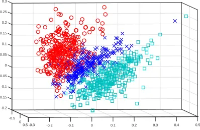
respectively. The dimensionality of the parametric model and the text vector both are reduced to 3 for visualization. It can be observed that points in Fig. 6 are more easily classified than those in Fig. 7, which demonstrates the effectiveness of our method of text representation.
0.5 0.4 0.3 0.2 0.1 0 -0.1 -0.2 0.5-0.3 0 -0.5 -0.2 0.05
-0.15 -0.1 -0.05 0 0.3
[image:11.612.329.539.226.373.2]0.1 0.15 0.2 0.25
Fig. 6. Visualization of three classes of the BBC news in LTTR
1 0.5 0 -0.5 0.5 0.4 0.3 0.2 0.1 0 -0.1 -0.2 -0.3 -0.4 -0.5 -0.3 0.4
0.3
0.2
0.1
0
-0.1
[image:11.612.68.267.295.424.2]-0.2
Fig. 7. Visualization of three classes of the BBC news in word2vec
As stated in Section III. The assumption of our method is that words from the same topic follow a Gaussian distribution. To show the ability of Gaussian mixture model for describ-ing the distribution of words, several words from six topics {economy,internet,language,social,sports,science}in Table VI are selected. The principal component analysis (PCA) is also used for visualization. Fig. 8 shows the distributions of words from different topics. The dimension of word vector has been reduced to two by PCA. It can be observed that
−0.4 −0.2 0 0.2 0.4 0.6
−0.8 −0.6 −0.4 −0.2 0 0.2 0.4 0.6 0.8
economy internet language social sports science linguistics
Fig. 8. Distributions of words from different topics with PCA visualization
these six topics are clearly separated. The word marked as ‘linguistics’ is most likely to belong to the ‘science’ topic, but it also appears in texts with topic ‘language’. So this word is located in both topics. This example validates the effectiveness of using a Gaussian mixture model to extract the topic diversity from words or texts.
E. The Results for Topic Coherence
In order to quantitatively analyze the quality of the topic-word learned by our method, the normalized Point-wise Mu-tual Information (PMI) [43] of topic words is used to measure the semantic coherence (topic coherence) of topic words. The co-occurrence statistics of topic words are extracted from Wikipedia, and then the normalized PMI score of a topic is computed by averaging the scores of the top 10 words of this topic on the 20newsgroup dataset. A higher normalized PMI score means a more semantically coherent topic [40].
[image:11.612.70.270.480.602.2]TABLE VIII
TOP WORDS OF SOME TOPICS AND NORMALIZEDPMIOF OUR METHOD
ANDLDAON20NEWSGROUP DATASET. THE WORDS OF OUR METHOD
ARE RANKED BASED ON THEIR PROBABILITY DENSITY IN EACH TOPIC. WORDS IN EACH COLUMN REPRESENT A TOPIC.
game president god university windows space gun
team government jesus institute file earth force
hockey people christian study dos orbit warning
play states man conference window space fire
Our method games money bible science program moon guns
nhl state christ technology server launch control
season public church information files flight guns
win rights christians engineering run mars police
pit clinton faith department problem astronomy weapons
period policy christianity college system satellites attack
normalized PMI 0.1083 0.1450 0.2233 0.1035 0.1050 0.1671 0.1039
year people god university window space gun
writes president jesus information image nasa people
game mr people national color gov law
good don bible research file earth guns
LDA model team money christian center windows launch don
article government church april program writes state
baseball stephanopoulos christ san display orbit crime
don time christians number jpeg moon weapons
games make life year problem satellite firearms
season clinton time conference screen article police
normalized PMI 0.0350 -0.0730 0.1451 0.0598 0.0810 0.1060 0.0812
V. CONCLUSION
In this paper, we propose a novel and efficient model to represent text and measure the distance between text rep-resentations by using a statistical manifold. Based on the distributional semantics hypothesis, we assume that words in the same topic follow a Gaussian distribution. Then we utilize a Gaussian mixture model to describe the distribution of all word vectors. The text representation is constructed from the perspective of text generation: text is generated from different topics. Hence the word space in a text is a subspace of all words. A modified Gaussian mixture model is used to represent texts according to their topics. The weight coefficient is re-calculated by the probability that the word belongs to each topic. As discussed in Section III, the computation complexity of giving a text representation is linearly related to the size of the text after constructing words label list.
After a discussion and analysis of distance metric between probability distributions, we chose a distance metric using statistical manifold learning. In a statistical manifold, each probability distribution that represents the text becomes a point on the manifold. In this perspective, metrics between probabil-ity distributions are defined from information geometry. This method can give the similarity result with a 2-norm distance defined in functional space. To demonstrate the effectiveness of our method, several state-of-the-art methods were used to compare with LTTR. The experimental results demonstrate the superiority of LTTR in terms of text representation and categorization. To illustrate the result of LTTR, the PCA has been used to visualize the distribution of text representations. To quantitatively analyze the topic coherence of LTTR, the normalized PMI has been employed to measure the semantic coherence of topic words.
Thus, our method solves practical problems in text repre-sentation and categorization. As future work, we will plan to provide more theoretical analysis and perform further experimental studies to demonstrate the effectiveness of our method. We also plan to extend our method to deal with text categorization problems in the field of semi-supervised
learning [44]–[46]. Besides, instead of using the Gaussian mixture model to describe the distribution of topics, there should be other effective probability models to make the metrics with statistical manifold learning be more stable and efficient.
REFERENCES
[1] H. Lodhi, C. Saunders, J. Shawe-Taylor, N. Cristianini, and C. Watkins, “Text classification using string kernels,”Journal of Machine Learning Research, vol. 2, pp. 419–444, 2002.
[2] G. Salton and C. Buckley, “Term-weighting approaches in automatic text retrieval,”Information Processing and Management, vol. 24, no. 5, pp. 513–523, 1988.
[3] B. Tang, S. Kay, and H. He, “Toward optimal feature selection in naive bayes for text categorization,”IEEE Transactions on Knowledge and Data Engineering, vol. 28, no. 9, pp. 2508–2521, 2016.
[4] M. J. Kusner, Y. Sun, N. I. Kolkin, and K. Q. Weinberger, “From word embeddings to document distances,” inProceedings of the International Conference on Machine Learning, 2015, pp. 957–966.
[5] T. Mikolov, K. Chen, G. Corrado, and J. Dean, “Efficient estimation of word representations in vector space,”Computer Science, 2013. [6] Q. V. Le and T. Mikolov, “Distributed representations of sentences and
documents,” inProceedings of the International Conference on Machine Learning, 2014, pp. 1188–1196.
[7] Y. Liu, Z. Liu, T.-S. Chua, and M. Sun, “Topical word embeddings,” inProceedings of the AAAI Conference on Artificial Intelligence, 2015, pp. 2418–2424.
[8] M. Rosen-Zvi, T. Griffiths, M. Steyvers, and P. Smyth, “The author-topic model for authors and documents,” inProceedings of the Conference on Uncertainty in Artificial Intelligence, 2004, pp. 487–494.
[9] L. Hennig and D. Labor, “Topic-based multi-document summarization with probabilistic latent semantic analysis.” inProceedings of the Recent Advances in Natural Language Processing, 2009, pp. 144–149. [10] D. M. Blei, A. Y. Ng, and M. I. Jordan, “Latent dirichlet allocation,”
Journal of Machine Learning Research, vol. 3, pp. 993–1022, 2003. [11] R. Das, M. Zaheer, and C. Dyer, “Gaussian lda for topic models with
word embeddings,” inProceedings of the Association for Computational Linguistics, 2015, pp. 795–804.
[12] P. Hu, W. Liu, W. Jiang, and Z. Yang, “Latent topic model based on gaussian-lda for audio retrieval,” in Proceedings of the Chinese Conference on Pattern Recognition, 2012, pp. 556–563.
[13] T. Luong, R. Socher, and C. D. Manning, “Better word representations with recursive neural networks for morphology.” in Proceedings of Conference on Computational Natural Language Learning, 2013, pp. 104–113.
[14] R. Socher, C. C. Lin, C. Manning, and A. Y. Ng, “Parsing natural scenes and natural language with recursive neural networks,” inProceedings of the International Conference on Machine Learning, 2011, pp. 129–136. [15] S. Lai, L. Xu, K. Liu, and J. Zhao, “Recurrent convolutional neural networks for text classification.” inProceedings of the AAAI Conference on Artificial Intelligence, 2015, pp. 2267–2273.
[16] K. Greff, R. K. Srivastava, J. Koutn´ık, B. R. Steunebrink, and J. Schmid-huber, “Lstm: A search space odyssey,”IEEE Transactions on Neural Networks and Learning Systems, vol. 28, no. 10, pp. 2222–2232, 2017. [17] R. Collobert, J. Weston, L. Bottou, M. Karlen, K. Kavukcuoglu, and P. Kuksa, “Natural language processing (almost) from scratch,”Journal of Machine Learning Research, vol. 12, pp. 2493–2537, 2011. [18] R. Socher, A. Perelygin, J. Y. Wu, J. Chuang, C. D. Manning, A. Y. Ng,
and C. Potts, “Recursive deep models for semantic compositionality over a sentiment treebank,” inProceedings of the Conference on Empirical Methods in Natural Language Processing, 2013, pp. 1631–1642. [19] K. Sun and S. Marchand-Maillet, “An information geometry of statistical
manifold learning,” inProceedings of the International Conference on Machine Learning, 2014, pp. 1–9.
[20] Z. S. Harris, “Distributional structure,”Word, vol. 10, no. 2-3, pp. 146– 162, 1954.
[21] L. Wolf, Y. Hanani, K. Bar, and N. Dershowitz, “Joint word2vec networks for bilingual semantic representations,”International Journal of Computational Linguistics and Applications, vol. 5, no. 1, pp. 27–44, 2014.
[23] T. Lin and H. Zha, “Riemannian manifold learning,”IEEE Transactions on Pattern Analysis and Machine Intelligence, vol. 30, no. 5, pp. 796– 809, 2008.
[24] G. Guo, Y. Fu, C. R. Dyer, and T. S. Huang, “Image-based human age estimation by manifold learning and locally adjusted robust regression,” IEEE Transactions on Image Processing, vol. 17, no. 7, pp. 1178–1188, 2008.
[25] C. Bregler and S. M. Omohundro, “Nonlinear manifold learning for vi-sual speech recognition,” inProceedings of the International Conference on Computer Vision, 1995, pp. 494–499.
[26] F. Cuzzolin and M. Sapienza, “Learning pullback hmm distances,”IEEE Transactions on Pattern Analysis and Machine Intelligence, vol. 36, no. 7, pp. 1483–1489, 2014.
[27] M. Balasubramanian and E. L. Schwartz, “The isomap algorithm and topological stability,”Science, vol. 295, no. 5552, p. 7, 2002. [28] S. T. Roweis and L. K. Saul, “Nonlinear dimensionality reduction by
locally linear embedding,”Science, vol. 290, no. 5500, pp. 2323–2326, 2000.
[29] S. S. Ho, P. Dai, and F. Rudzicz, “Manifold learning for multivariate variable-length sequences with an application to similarity search,”IEEE Transactions on Neural Networks and Learning Systems, vol. 27, no. 6, pp. 1333–1344, 2016.
[30] X. Xu, Z. Huang, L. Zuo, and H. He, “Manifold-based reinforcement learning via locally linear reconstruction,”IEEE Transactions on Neural Networks and Learning Systems, vol. 28, no. 4, pp. 934–947, 2017. [31] C. M. Bishop, Pattern recognition and machine learning. Springer,
2006.
[32] L. Bai and E. R. Hancock, “Graph kernels from the jensen-shannon divergence,”Journal of Mathematical Imaging and Vision, vol. 47, no. 1-2, pp. 60–69, 2013.
[33] D. Polani, “Kullback-leibler divergence,” in Encyclopedia of Systems Biology, 2013, pp. 1087–1088.
[34] S. J. Julier and J. K. Uhlmann, “A general method for approximating nonlinear transformations of probability distributions,” Robotics Re-search Group, Department of Engineering Science, University of Oxford, Oxford, OC1 3PJ United Kingdom, Tech. Rep, 1996.
[35] J. R. Hershey and P. A. Olsen, “Approximating the kullback leibler divergence between gaussian mixture models,” in Proceedings of the International Conference on Acoustics, Speech and Signal Processing, 2007, pp. 317–320.
[36] M. Suzuki, “Information geometry and statistical manifold,” arXiv preprint arXiv:1410.3369, 2014.
[37] N. H. Abdel-All, H. Abd-Ellah, and H. Moustafa, “Information geometry and statistical manifold,”Chaos, Solitons and Fractals, vol. 15, no. 1, pp. 161–172, 2003.
[38] T. Jaakkola and D. Haussler, “Exploiting generative models in dis-criminative classifiers,” inAdvances in Neural Information Processing Systems, 1999, pp. 487–493.
[39] L. Maaten, “Learning discriminative fisher kernels,” inProceedings of the International Conference on Machine Learning, 2011, pp. 217–224. [40] O. Levy, Y. Goldberg, and I. Dagan, “Improving distributional similarity with lessons learned from word embeddings,” Transactions of the Association for Computational Linguistics, vol. 3, pp. 211–225, 2015. [41] M. Steyvers and T. Griffiths, “Probabilistic topic models,”Handbook of
Latent Semantic Analysis, vol. 427, no. 7, pp. 424–440, 2007. [42] T. F. Y. Lam Hong Lee, Chin Heng Wan and H. M. Kok, “A review of
nearest neighbor-support vector machines hybrid classification models,” Journal of Applied Sciences, no. 10, pp. 1841–1858, 2010.
[43] J. H. Lau, D. Newman, and T. Baldwin, “Machine reading tea leaves: Automatically evaluating topic coherence and topic model quality.” in Proceedings of the Conference of the European Chapter of the Association for Computational Linguistics, 2014, pp. 530–539. [44] B. Jiang, H. Chen, B. Yuan, and X. Yao, “Scalable graph-based
semi-supervised learning through sparse bayesian model,”IEEE Transactions on Knowledge and Data Engineering, vol. 29, no. 12, pp. 2758–2771, 2017.
[45] O. Chapelle, B. Sch¨olkopf, and A. Zien, Semi-Supervised Learning. MIT Press Cambridge, 2006.
[46] R. Johnson and T. Zhang, “Supervised and semi-supervised text cat-egorization using lstm for region embeddings,” inProceedings of the International Conference on Machine Learning, 2016, pp. 526–534.
Bingbing Jiang received the B.Sc degree from Chongqing University of Posts and Telecommuni-cations (CQUPT), Chongqing, China, in 2014. He is currently working toward the Ph.D degree in the School of Computer Science and Technology, University of Science and Technology of China (USTC), Hefei, China. His research interests include Sparse Bayesian learning, semi-supervised learning, feature selection and text categorization.
Zhengyu Li received the B.Sc and M.Sc degrees in computer science from University of Science and Technology of China (USTC), Hefei, China, in 2014 and 2017, respectively. He is currently a research assistant in Advertisement Research for Sponsored search (ADRS) group in Sogou Inc. His research interests include query intent detection, sentiment analysis, short text clustering, topic modeling, and their applications in sponsored search.
Huanhuan Chen(M’09–SM’16) received the B.Sc degree from the University of Science and Tech-nology of China (USTC), Hefei, China, in 2004 and the Ph.D degree in computer science from the University of Birmingham, Birmingham, UK, in 2008. He is currently a Full Professor in the School of Computer Science and Technology, USTC. His research interests include neural networks, Bayesian inference and evolutionary computation. Dr. Chen received the 2015 International Neural Network Society Young Investigator Award, the 2012 IEEE Computational Intelligence Society Outstanding Ph.D. Dissertation Award, the IEEE TRANSACTIONS ON NEURAL NETWORKS Outstanding Paper Award (bestowed in 2011 and only one paper in 2009), and the 2009 British Computer Society Distinguished Dissertations Award. He is an Associate Editor of the IEEE TRANSACTIONS ON NEURAL NETWORKS AND LEARNING SYSTEMS, and the IEEE TRANSACTIONS ON EMERGING TOPICS IN COMPUTATIONAL INTELLIGENCE.