Solving the Multiple-Instance Problem:
A Lazy Learning Approach
Jun Wang [email protected]
Institute of Computing Technology, Chinese Academy of Sciences, Beijing 100080 China
Graduate School of Library and Information Science, University of Illinois at Urbana-Champaign, Champaign, IL 61820 USA
Jean-Daniel Zucker [email protected]
LIP6-CNRS, University Paris VI 4, Place Jussieu, F-75252, Paris Cedex 05 France
Abstract
As opposed to traditional supervised learning, multiple-instance learning concerns the problem of classifying a bag of instances, given bags that are labeled by a teacher as being overall positive or negative. Current research mainly concentrates on adapting traditional concept learning to solve this problem. In this paper we investigate the use of lazy learning and Hausdorff distance to approach the multiple-instance problem. We present two variants of the K-nearest neighbor algorithm, called Bayesian-KNN and Citation-KNN, solving the
multiple-instance problem. Experiments on the Drug discovery benchmark data show that both algorithms are competitive with the best ones conceived in the concept learning framework. Further work includes exploring of a combination of lazy and eager multiple-instance problem classifiers.
1.
Introduction
The multiple-instance problem or multiple-instance
learning is receiving growing attention in the machine
learning research field (Dietterich, Lathrop, & Lozano-Pérez, 1997; Zucker & Ganascia, 1996; Auer, 1997; Blum & Kalai, 1998; Maron, 1998; De Raedt, 1998; Ruffo, 2000). Most of the work in machine learning is focused on supervised learning where each example is labeled by a teacher. In multiple-instance learning, the teacher labels examples that are sets (also called bags) of instances. The teacher does not label whether an individual instance in a bag is positive or negative. The learning algorithm needs to generate a classifier that will classify unseen examples (i.e. bags of instances) correctly.
Dietterich et al. (1994) encountered this problem in the task of classifying aromatic molecules according to
whether or not they are "musky". Several steric (i.e., "molecular shape") configurations of the same molecule can be found in nature, each with very different energy properties. In this way it is possible to produce several descriptions of the different configurations – instances – of this molecule. These descriptions correspond to measurements obtained in each of the different configurations. To simplify, a molecule is said to be musky if, in one of its configurations, it binds itself to a particular receptor. The problem of learning the concept "musky molecule" is one of the multiple-instance problems. Maron and Ratan (1998) considered other possible applications: one is to learn a simple description of a person from a series of images that are labeled positive if the person is somewhere in the image and negative otherwise. There are also promising data mining applications for this setting (Ruffo, 2000).
description used in the inductive logic programming (ILP) (Zucker & Ganascia, 1996; De Raedt, 1998; Blockeel & De Raedt, 1998; Zucker & Ganascia, 1998; Sebag & Rouveirol, 1998).
Lazy learning is the framework in which training examples are simply stored for future use rather than used to construct general, explicit description of the target function. Typical types of lazy learning are instance-based, case-instance-based, memory-instance-based, exemplar-instance-based, and experience-based learning (Aha, 1997). Dietterich et al. (1994) were the first ones to apply the K-nearest neighbor
(KNN) algorithm (the most widely used method in lazy learning (Dasarathy, 1991)) to attack the drug discovery problem. However, their purpose was to show that nearest neighbor methods with Euclidean distance and tangent distance were worse than neural network with dynamic reposing in the feature manifold problem.
The motivation of the present study is to investigate the issues raised by introducing lazy learning approaches such as KNN to deal with the multiple-instance problem and evaluate the interest of using lazy learning. In fact, using Hausdorff distance (Edgar, 1995) does allow KNN algorithms to be adapted to the multiple-instance problem. Our experiments show that the two general-purpose algorithms we devised – Bayesian-KNN and Citation-KNN
– did reach the best results obtained so far by ad-hoc algorithms on the drug discovery task. These good results obtained may indicate that the multiple-instance problem (at least in the drug discovery problem) is well fitted to
local approaches (Bottou & Vapnik, 1992), which yield
highly adaptive behavior not usually found in concept learning. It also suggests that combining lazy learning with concept learning classifiers could possibly lead to better prediction accuracy than any other existing method.
Section 2 defines the semantics of nearest neighbor learning in the multiple-instance learning context and introduces a modified version of Hausdorff distance. Section 3 presents the basis for adapting KNN algorithms to the multiple-instance problem. Section 4 details experimental evaluation and comparison with existing learning algorithms. The last section is dedicated to discussion and future work.
2.
Using Hausdorff Distance in the Lazy
Learning Setting
Different approaches have been adopted to classify an unseen bag of instances in the context of multiple-instance problem. The first approach consists in classifying as positive a bag if at least one of its instances belongs to the learned concept and negative otherwise (Dietterich et al., 1997). Another approach implemented in RELIC consists in making the different instances of a bag vote for the class of the bag (Ruffo, 2000). Finally, if a bag is considered as a particular kind of relational data, classification techniques in classical structural learning
(Bergadano, Giordana, & Saitta, 1991) or inductive logic programming (De Raedt, 1998) may be used.
In lazy learning, the class of a test example is computed by combining the classes of training examples. In KNN, the class values of the K nearest neighbors of the considered test example are combined. This algorithm assumes that all examples correspond to points in an n-dimensional space, and the nearest neighbors of an example are defined in terms of standard Euclidean distance.
However, in the context of the multiple-instance problem, an example is a bag that contains multiple instances and therefore does not correspond to a single point. In order to define a distance between bags we need to characterize how the distance between two sets of instances could be measured. The Hausdorff distance provides such a metric function between subsets of a metric space. By definition, two sets A and B are within Hausdorff distance d of each other iff every point of A is within distance d of at least one point of B, and every point of B is within distance d of at least one point of A (Edgar, 1995).
Formally speaking, given two sets of points A={a1,…,am}
and B={b1,…,bn}, the Hausdorff distance is defined as:
)}
,
(
),
,
(
max{
)
,
(
A
B
h
A
B
h
B
A
H
=
where
b
a
B
A
h
B b A
a
−
=
∈ ∈
min
max
)
,
(
.For example, let A={1,2,3} and B={4,5,6}, and the ||a-b|| is defined as |a-b|. Thus h(A,B)=max{|1-4|, |2-4|, |3-4|} =3, and h(B,A)=max{|4-3|, |5-3|, |6-3|}=3. Then the H(A,B) = max{h(A,B), h(B,A)} = 3.
The Hausdorff distance is very sensitive to even a single outlying point of A or B. For example, consider
B={4,5,20}, where the 20 is some large distance away
from every point of A. In this case, H(A,B)=|20-3|=17, which means that the distance is solely determined by this outlying point.
To increase the robustness of this distance with respect to noise, we shall thus consider a modification of the Hausdorff distance. This modified measure is given by taking the k-th ranked distance rather than the maximum, or the largest ranked one,
b
a
kth
B
A
h
B b A a
k
(
,
)
=
∈min
∈−
where kth denotes the k-th ranked value. When k=m, kth reaches its maximum value, and thus the distance is the same as h(A,B) defined above. We call hm(.,.)=h(.,.) the
maximal Hausdorff distance. When k=1, the minimal one
of the m individual point distances decides the value of the overall distance. Since
)
,
(
min
min
min
min
)
,
(
11
A
B
a
b
a
b
h
B
A
h
A a B b B
b A
a
−
=
−
=
=
∈ ∈ ∈
thus in this case, H(A,B)=h1(A,B)=h1(B,A). We call this
measure the minimal Hausdorff distance. We suggest in this paper using this modified Hausdorff distance as a basis for adapting KNN to the multiple-instance problem. For the sake of clarity, only the minimal Hausdorff distance will be used in the next section. Nevertheless, the experiment section presents results that are based on both the maximal and the minimal Hausdorff distance.
3.
Adapting
K-Nearest Neighbor to the
Multiple-Instance Problem
3.1 A Contradiction: Minor Being Winner
Based on the minimal Hausdorff distance between bags, we applied the conventional KNN method to the multiple-instance problem in the Musk1 data set in the drug discovery application (from the UCI repository). There are 47 positive bags and 45 negative in the Musk1 data set (see section 4.1 for more detail). According to the KNN method, the class value of an unseen bag is the most common class of its nearest training bags. Thus, assuming the classes of its three (K=3) nearest neighbors are {P,P,N} (P stands for positive and N for negative), then its class will be predicted to be P. However, this prediction strategy appeared not to be optimal. In fact, using the Hausdorff distance was not sufficient to adapt KNN to the multiple-instance problem.
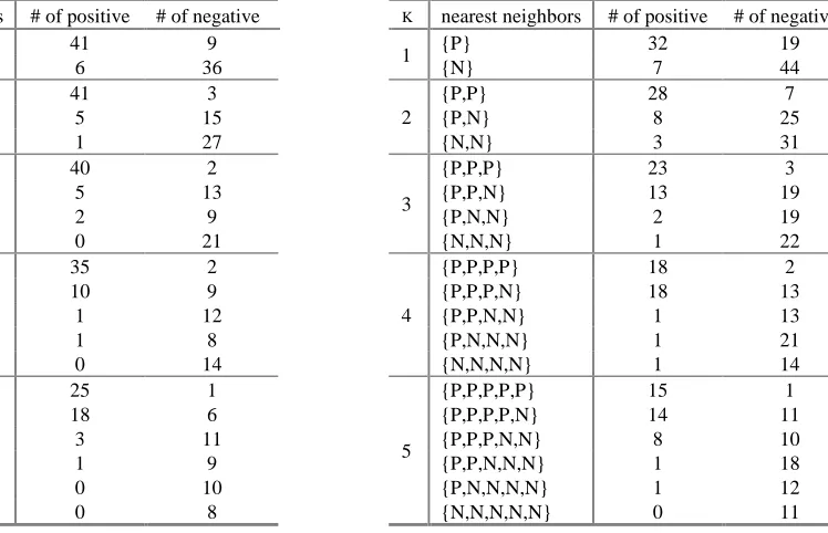
Table 1. Class distribution of the K nearest neighbors of the positive/negative bags on the Musk1 data set. The third/fourth column means the number of positive/negative bags whose K nearest neighbors have the class set in the second column.
K K nearest
neighbors
number of positive
number of
negative sum
{P} 41 9 50
1
{N} 6 36 42
{P,P} 41 3 44
{P,N} 5 15 20
2
{N,N} 1 27 28
{P,P,P} 40 2 42
{P,P,N} 5 13 18
{P,N,N} 2 9 11
3
{N,N,N} 0 21 21
Table 1 shows the class distribution of the nearest neighbors of negative or positive bags. The table also shows a seemly contradictory case. When K=3, there are 18 bags whose K nearest neighbors have the classes {P,P,N}. Among these 18 bags, thirteen are negative and five are positive. This observation indicates that for an unseen bag whose three nearest neighbors have the classes {P,P,N}, if it is predicted as negative rather than positive, the overall prediction accuracy will be much higher.
In traditional supervised learning, the contradiction will not happen. The contradiction in multiple-instance learning may be explained by the fact that positive bags contain "true positive instances" as well as "false positive instances", and the latter may attract negative bags. A simple illustration may clarify this particular case (see Figure 1). Given {P1, P2, N1} as three training bags, N2 will be classified as positive. Given {N1, N2, P1} as three training bags, P2 will be classified as negative.
P
1P
2Feature2
Feature 1
N
1N
2false positive instances
Figure 1. The instances of each negative bag are represented as
aligned round dots, and the instances of each positive bag as aligned square blocks.
There are several ways to avoid this classification problem. One way is to modify the definition of bag distance so as to take the problem into account (i.e., using a weighted Hausdorff distance). Table 1 suggests that in a multiple-instance setting negative bags should be weighed more than positive ones. Table 8 (in Appendix) gives a more detailed analysis of the class distribution of K nearest neighbors on the Musk1 and Musk2 data sets. It shows that the contradiction also occurs for values of K greater than three. Another way to cope with the classification problem mentioned above is to consider new methods about how to combine the nearest bags to derive a better result. In this paper we will take the second approach for the purpose of evaluating the benefits of using straightforward adaptation of KNN methods to the multiple-instance problem.
3.2 A Bayesian Approach
One way to overcome the above classification problem is to use a Bayesian approach. Let us first examine the typical majority vote method as introduced in the previous section and then introduce a Bayesian version of it. For an unseen bag b, assume its K nearest bags are {b1,b2,…,bk},
and their classes are respectively {c1,c2,…,ck}, where ci is
either positive or negative. If we use the majority vote to determine the class of b, then the result will be:
∑
= ∈
k
i
i negative
positive c
c
c
1 } , {
)
,
(
max
arg
δ
The aforementioned contradiction tells us that the majority vote approach does not always provide the best prediction result. Bayesian method provides a probabilistic approach that calculates explicit probabilities for hypotheses. For each hypothesis c that the class of b can take, the posterior probability of c is p(c|{c1,c2, …,
ck}). We are interested in finding the most probable
hypothesis c∈{positive, negative} given the observed data {c1,c2,…,ck}. According to Bayes theorem, the maximally
probable hypothesis is:
)
(
)
|
}
,...,
,
({
max
arg
})
,...,
,
({
)
(
)
|
}
,...,
,
({
max
arg
})
,...,
,
{
|
(
max
arg
2 1
2 1 2 1
2 1
c
p
c
c
c
c
p
c
c
c
p
c
p
c
c
c
c
p
c
c
c
c
p
k c
k k
c
k c
=
=
Since ci is either positive or negative, the maximal
number of combination that {c1,c2,…,ck} can take is k+1,
the computational cost of this measure is therefore not expensive. This algorithm is called Bayesian-KNN, and its
performances are presented in section 4.
3.3 A Citation Approach
Another way to adapt KNN to the multiple-instance problem was inspired to us by the notion of citation from library and information science (Garfield, 1979). In this domain, finding related documents (especially research papers) is an important research topic. One well-known method is based on references and citers. If a research paper does cite another previously published paper (as known as its reference), the paper is said to be related to the reference. Similarly, if a paper is cited by a subsequent article (as known as its citer), the paper is also said to be related to its citer. Therefore, both citers and references are considered to be candidate documents related to a given paper.
What suggests the notion of citation is to take not only into account the neighbors of a bag b (according to the Hausdorff distance) but also the bags that count b as a neighbor. We could use either references or citers of an unseen example to predict the class of the example rather than only use the references. It is easy to define the R -nearest references of an example b as the R-nearest neighbors of b. However, it is a little more complex to define the citers of an example. Let n be the number of all example bags BS={b1, …, bn}, then for an example b∈BS,
all other examples BS\b={bi | bi∈BS, bi≠b} can be ranked
according to the similarity to the example b. For b'∈BS\b,
let its rank number be Rank(b',b). For the sake of completeness, let us set Rank(b,b) to be ∞. Now, for any example b in BS, we define the C-nearest citers of b as Citers(b, C)={bi|Rank(bi,b)≤C, bi∈BS}. (It should be noted
that we could also define C-nearest citers according to distance rather than rank.)
For example, assuming that there are only 6 bags of instances {b1,b2,b3,b4,b5,b6} in a data set. Their nearest neighbors are shown in Table 2. Let both R and C be 2, then for the bag b1, its R-nearest references are {b3,b2}, and its C-nearest citers are {b2,b3,b5}.
Table 2. The nearest neighbors of 6 bags {b1,b2,b3,b4,b5,b6}. N
means the nearest rank number.
N=1 N=2 N=3 N=4 N=5
b1 b3 b2 b5 b4 b6
b2 b1 b4 b5 b3 b6
b3 b5 b1 b2 b6 b4
b4 b6 b2 b1 b3 b5
b5 b1 b2 b3 b6 b4
b6 b4 b3 b1 b2 b5
Let us now concentrate on how to combine the R-nearest references and the C-nearest citers of an unseen bag b to derive its class. Assume that for the R-nearest references, the numbers of positive and negative bags are Rp and Rn respectively; and for the C-nearest citers, the numbers of positive and negative bags are Cp and Cn respectively (see Table 3).
Table 3. Distribution of positive and negative bags in R-nearest references and C-nearest citers of an unseen bag.
positive bags negative bags
R-nearest
references Rp Rn R
C-nearest
citers Cp Cn C
p=Rp+Cp n=Rn+Cn
Let p=Rp+Cp , and n=Rn+Cn. We called Citation-KNN the KNN algorithm in which p and n are computed by using the Hausdorff distance and classification is defined as follows: if p>n, then the class of the bag b is predicted as positive, otherwise negative. It should be noted that when a tie happens, the class of b is set to be negative (see section 3.1 for detailed reasons). The performances of Citation-KNN are presented in the following section.
4.
Experimental Space Evaluation
4.1 The Musk Data Sets
sets are shown in Table 4. Each instance (conformation) has 166 numerical attributes.
Table 4. Some characteristics of the two Musk data sets.
Data set Musk1 Musk2
# of bags 92 102
# of positive bags 47 39
# of negative bags 45 63
average # of instances per bag 5.2 64.7
average # of instances per positive bag 4.4 26.1
average # of instances per negative bag 6.0 88.6
4.2 Experimental Method
We ran Bayesian-KNN and Citation-KNN on Musk1 and Musk2 for different values of K or R and the two Hausdorff distance methods: minimal Hausdorff distance (briefly called minHD) and maximal Hausdorff distance (briefly called maxHD). Since each instance is a point in 166-dimensional real-valued Euclidean space, the distance between two instances is calculated in Euclidean distance.
We report experimental results using the leave-one-out test to predict accuracy rather than using the 10-fold or 20-fold cross validation. One reason is that to date the best prediction accuracy acquired by "iterated-discrim APR" (Dietterich et al., 1997) was tested implicitly using the leave-one-out. Another reason is that there is no variation for this test method although usually the difference between the leave-one-out and the 10-fold or 20-fold is not significant.
4.3 Experimental Results
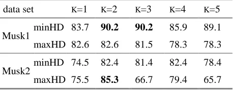
For Bayesian-KNN algorithm, the experimental result is shown in Table 5 for different values of K and the two kinds of Hausdorff distance. With the Musk1 data set, the minimal Hausdorff distance method acquired the best prediction accuracy 90.2%. With the Musk2 data set, the maximal Hausdorff distance method performs the best (85.3%), but when K>2 it is worse than the minimal method. On the whole, when K=2 the results are the best.
Table 5. Bayesian-KNN prediction accuracy in % for different K and the two kinds of Hausdorff distance: minHD and maxHD.
data set K=1 K=2 K=3 K=4 K=5
minHD 83.7 90.2 90.2 85.9 89.1
Musk1
maxHD 82.6 82.6 81.5 78.3 78.3
minHD 74.5 82.4 81.4 82.4 78.4
Musk2
maxHD 75.5 85.3 66.7 79.4 65.7
Table 6. Citation-KNN prediction accuracy in % on different R and the two kinds of Hausdorff distance: minHD and maxHD.
data set R=0 R=1 R=2 R=3 R=4
minHD 84.8 87.0 92.4 92.4 83.7
Musk1
maxHD 78.3 84.8 84.8 84.8 83.7
minHD 83.3 78.4 86.3 83.3 83.3
Musk2
maxHD 84.3 80.4 85.3 82.4 79.4
For Citation-KNN algorithm, the result is shown in Table 6 for different values of R and the two kinds of Hausdorff distance. The value of C was empirically set to be R+2 so
as to reflect that citers seem to be more important than references. Generally, the minimal Hausdorff distance method performs better than the maximal one, and when R=2 the results are the best.
Results on the Musk1 and Musk2 data sets suggests that while the two methods appear to work well when there are not too many instances per bag (as in Musk1), they seem insufficient with many instances per bag (as in Musk2). One possible explanation is that positive bags contain "false positive instances", and negative bags in Musk2 contain much more instances than Musk1, therefore the "false positive instances" in Musk2 are easier to be trapped by negative bags. One possible solution might be to remove those false positive instances from the positive bags and to recalculate the Hausdorff distance between those bags.
4.4 Comparison with Existing Algorithms
Table 7. Comparison of the prediction accuracy obtained with
Citation-KNN and Bayesian-KNN (only with minimal Hausdorff distance) with those of other systems on the Musk data sets.
Algorithms Musk1
%correct
Musk2 %correct
iterated-discrim APR 92.4 89.2
Citation-KNN 92.4 86.3
Bayesian-KNN 90.2 82.4
Diverse Density 88.9 82.5
RELIC 83.7 87.3
MULTINST 76.7 84.0
TILDE N/A 79.4
four APR algorithms reported in Dietterich et al. (1997). MULTINST algorithm is taken from Auer (1997), and Diverse Density algorithm from Maron & Lozano-Pérez (1998). TILDE is a top-down induction system for learning first order logical decision tree (Blockeel & De Raedt, 1998). The Musk data set being totally numerical is not a typical ILP task, which explains the result of TILDE. RELIC is an efficient top-down induction system that extends C4.5 so as to learn multiple-instance decision trees (Ruffo, 2000).
4.5 Discussion
Citation-KNN did quite well on both data sets. On average it is only worse than the best one "iterated-discrim APR". However, the high accuracy of the latter on Musk2 is partly due to the fact that some of its parameters were set based on the experiments on the Musk1 data set. In fact, the APR algorithm was designed with the drug discovery problem in mind, it is unclear whether it will generalize well to other problems or not. In contrast, Citation-KNN and Bayesian-KNN algorithms are general-purpose and effective.
Although the two adaptation algorithms of KNN to the multiple-instance problem performed remarkably well, the basic reasons why they acquired such high accuracy on the Musk data sets are unclear. It is also not clear whether they are fit for other multiple-instance learning applications such as stock prediction (not available publicly) and image retrieval (Maron, 1998). It should finally be noted that, as opposed to our algorithms, both ILP systems RELIC and TILDE produce comprehensible results. Moreover, they are also directly applicable on symbolic data.
5.
Conclusion and Future Work
The motivation of our work is to investigate the devising of lazy learning algorithms to attack the multiple-instance problem. Results of the experimental comparison show that using a modified version of Hausdorff distance for adapting the KNN algorithm to the multiple-instance problem led to high performance in the drug discovery task, competitive with that of algorithms developed within the concept learning framework. Two kinds of adaptation of KNN were proposed in this paper, a Bayesian one (Bayesian-KNN) and another based on the notion of citation (Citation-KNN). Experimental results on the Musk data sets show that the multiple-instance problem (at least in the drug discovery task) may be solved by both concept learning and lazy learning. It is likely that combining both approaches would lead to an increase in prediction accuracy.
The two algorithms presented in this paper did not consider the curse of dimensionality, where many features are irrelevant to the performance task (the nearest neighbor algorithm is highly sensitive to this situation).
Both Dietterich et al. (1997) and Maron (1998) stated that the number of relevant features are much fewer than 166 – the number of all features. If a feature selection function was added as a preprocessing of the algorithms, it is also likely that better results would be obtained. Another promising direction is to consider other definitions of distance between bags. We are currently investigating how to recast our approach in the context of support vector machine (Vapnik, 1995). Support vectors could be used to measure the distance between two bags as the distance between support vectors from two bags. We are also investigating multicriteria analysis methods (Perny, 1998) to weigh the instances role in the classification decision. In the Citation-KNN algorithm, the importance of the relative numbers of citers and references needs also to be further explored.
Acknowledgements
This work is supported by a grant from the French government AFCRST-PRA-096. We are grateful to anonymous referees for their useful comments and suggestions on an earlier version of this paper.
References
Aha, D. W. (Ed.). (1997). Lazy Learning. Dordrecht, The Netherlands: Kluwer Academic Publishers.
Auer, P. (1997). On learning from multi-instance examples: Empirical evaluation of a theoretical approach. Proceedings of the Fourteenth International
Conference on Machine Learning (pp. 21–29). San
Francisco: Morgan Kaufmann.
Bergadano, F., Giordana, A., & Saitta, L. (1991).
Machine learning: An integrated framework and its application. Chichester, UK: Ellis Horwood.
Blockeel, H., & De Raedt, L. (1998). Top-down induction of first order logical decision trees. Artificial
Intelligence, 101, 285–297.
Blum, A., & Kalai, A. (1998). A note on learning from multiple-instance examples. Machine Learning, 30, 23– 29.
Bottou, P., & Vapnik, V. (1992). Local learning algorithms. Neural Computation, 4, 888–900.
Dasarathy, B.V. (1991). Nearest neighbor norms: NN
pattern classification techniques. Los Alamitos, CA:
IEEE Computer Society Press.
De Raedt, L. (1998). Attribute-value learning versus inductive logic programming: The missing links.
Proceedings of the Eighth International Conference on Inductive Logic Programming (pp. 1–8).
Dietterich, T.G., Jain, A., Lathrop, R. H., & Lozano-Pérez, T. (1994). A comparison of dynamic reposing and tangent distance for drug activity prediction.
Advances in Neural Information Processing Systems, 6,
216–223. San Mateo: Morgan Kaufmann.
Dietterich, T.G., Lathrop, R. H., & Lozano-Pérez, T. (1997). Solving the multiple-instance problem with axis-parallel rectangles. Artificial Intelligence, 89, 31– 71.
Edgar, G.A. (1995). Measure, topology, and fractal
geometry (3rd print). Springer-Verlag.
Garfield, E. (1979). Citation indexing: Its theory and
application in science, technology, and humanities.
New York: John Wiley & Sons.
Long, P.M., & Tan, L. (1996). PAC-learning axis aligned rectangles with respect to product distributions from multiple-instance examples. Proceedings of the Ninth
Annual Conference on Computational Learning Theory
(pp. 228–234). New York: ACM Press.
Maron. O., & Lozano-Pérez, T. (1998). A framework for multiple-instance learning. Advances in Neural
Information Processing Systems, 10. MIT Press.
Maron, O., & Ratan, A. L. (1998). Multiple-instance learning for natural scene classification. Proceedings of
the Fifteenth International Conference on Machine Learning. San Francisco: Morgan Kaufmann.
Maron, O. (1998). Learning from ambiguity. Doctoral dissertation, Department of Electrical Engineering and
Computer Science, Massachusetts Institute of Technology.
Perny, P. (1998). Multicriteria filtering methods based on concordance and non-discordance principles. Annals of
Operations Research, 80, 137–165. Bussum, The
Netherlands: Baltzer Science Publishers.
Ruffo, G. (2000). Learning single and multiple instance
decision tree for computer security applications.
Doctoral dissertation, Department of Computer Science, University of Turin, Torino, Italy.
Sebag, M., & Rouveirol, C. (1997). Tractable induction and classification in first order logic via stochastic matching. Proceedings of the Fifteenth International
Joint Conference on Artificial Intelligence (pp. 888–
893). Nagoya, Japan: Morgan Kaufmann.
Vapnik, V. (1995). The nature of statistical learning
theory. New York: Springer-Verlag.
Zucker, J.-D., & Ganascia, J.-G. (1996). Changes of representation for efficient learning in structural domains. Proceedings of the Thirteenth International
Conference on Machine Learning (pp. 543–551). Bary,
Italy: Morgan Kaufmann.
Zucker, J.-D., & Ganascia, J.-G. (1998). Learning structurally indeterminate clauses. Proceedings of the
Eighth International Conference on Inductive Logic Programming (pp. 235–244). Springer-Verlag.
Appendix
Table 8. Class distribution of K nearest neighbors of the positive/negative bags on the Musk1 (left) and Musk2 (right) data sets.
K nearest neighbors # of positive # of negative
{P} 41 9
1
{N} 6 36
{P,P} 41 3
{P,N} 5 15
2
{N,N} 1 27
{P,P,P} 40 2
{P,P,N} 5 13
{P,N,N} 2 9
3
{N,N,N} 0 21
{P,P,P,P} 35 2
{P,P,P,N} 10 9
{P,P,N,N} 1 12
{P,N,N,N} 1 8
4
{N,N,N,N} 0 14
{P,P,P,P,P} 25 1
{P,P,P,P,N} 18 6
{P,P,P,N,N} 3 11
{P,P,N,N,N} 1 9
{P,N,N,N,N} 0 10
5
{N,N,N,N,N} 0 8
K nearest neighbors # of positive # of negative
{P} 32 19
1
{N} 7 44
{P,P} 28 7
{P,N} 8 25
2
{N,N} 3 31
{P,P,P} 23 3
{P,P,N} 13 19
{P,N,N} 2 19
3
{N,N,N} 1 22
{P,P,P,P} 18 2
{P,P,P,N} 18 13
{P,P,N,N} 1 13
{P,N,N,N} 1 21
4
{N,N,N,N} 1 14
{P,P,P,P,P} 15 1
{P,P,P,P,N} 14 11
{P,P,P,N,N} 8 10
{P,P,N,N,N} 1 18
{P,N,N,N,N} 1 12
5