R E S E A R C H
Open Access
Iterative learning control for MIMO
parabolic partial difference systems with time
delay
Xisheng Dai
1*, Xuemin Tu
2, Yong Zhao
3, Guangxing Tan
1and Xingyu Zhou
1*Correspondence:
1School of Electrical and
Information Engineering, Guangxi University of Science and Technology, Liuzhou, China Full list of author information is available at the end of the article
Abstract
In this paper, the iterative learning control (ILC) technique is extended to multi-input multi-output (MIMO) systems governed by parabolic partial difference equations with time delay. Two types of ILC algorithm are presented for the system with state delay and input delay, respectively. The sufficient conditions for tracking error convergence are established under suitable assumptions. Detailed convergence analysis is given based on discrete Gronwall’s inequality and discrete Green’s formula for the systems with time-varying uncertainty coefficients. Numerical results show the effectiveness of the proposed ILC algorithms.
Keywords: Iterative learning control; Parabolic partial difference systems; Time delay; Convergence
1 Introduction
The system governed by partial difference equations is a class of important dynamic sys-tems which firstly arises as numerical solution of partial differential equations. In fact, the state space model of partial difference system can cover many nature laws, such as logis-tic model with spatial migration, mathemalogis-tics physical processes (discrete heat equation), engineering technology (image processing, digital signal processing, circuit systems) (see [1,2] and the references therein). There are many excellent results on the partial difference equations/systems, including exist/no exist [3,4], stability [5], oscillation [6], positivity of solutions [7], etc. From the view point of practicality, since the first step, that is, the im-plementation of control for distributed parameter systems modeled by partial differential equations, requires to discretize the variable of systems, studying the control of partial difference systems has a great value.
Iterative learning control (ILC) is an intelligent control method which imitates human learning behavior [8]. For a repeatable system in a given finite time interval, based on tracking objective and previous input and output information, ILC can improve the sys-tem performance with the increase in the iteration number. ILC algorithm is simple but it can deal with many complex systems with nonlinear and uncertain characteristics [9,10]. As an effective control algorithm, ILC has been used to track a given target in many types of systems, including ordinary difference/differential systems [11,12], partial differential systems or distributed parameter systems [13,14], impulsive systems [15], stochastic
tems [16], fractional systems [17], etc. However, there are few results on ILC for partial difference systems.
Motivated by the above, in this paper, we investigate the ILC problem of MIMO parabolic partial difference equations with delay. Both the P-type ILC scheme and ILC scheme with time delay parameter are proposed for systems with state delay and input delay, respectively. Convergence conditions are given by using a discrete form inequal-ity/formula. It is shown that selecting the learning gain parameter through the iterative learning process can guarantee the convergence of the output tracking error between the given desired output and the actual output.
Compared with the current literature, the main features of this work are summarized as follows: (1) It can handle MIMO parabolic partial difference systems. Although Refs. [18,
19] studied ILC for partial difference systems, the systems are only the single-input and single-output (SISO). Because a MIMO system often involves multi-input variables and multi-output variables, the input and output of a SISO system only are one, respectively, so the mathematical analysis of a MIMO system is more complex than that of a SISO system. (2) The systems include time delay in state and input. The ILC of systems with time delay is studied in [12,20], but the systems are stated by ordinary difference equations, which is different to this paper. The system in this paper is governed by partial difference equations and simultaneously involving three different indices: time, space, and iteration; therefore the convergence analysis is more complex. (3) We used the methods of partial difference equations which have been applied in stability analysis from partial difference systems [2,4–6], instead of Lyapunov method or linear matrix inequality (for multi dimensional dynamic systems) [21,22].
The rest of the paper is arranged as follows. In Sect.2, we present the formulation and some preliminaries. Section3provides ILC design and rigorous convergence analysis. In Sect.4, the simulation results are illustrated. Finally, the conclusions of this paper are shown in Sect.5.
2 ILC system description
In this paper, we consider the following two classes of parabolic type partial difference systems, which run a given task repeatedly on a finite time interval [0,J]. The first class is the system with time delay in state as follows:
⎧ ⎪ ⎪ ⎪ ⎨ ⎪ ⎪ ⎪ ⎩
2Zk(x,s) = D(s)12Zk(x– 1,s) + A(s)Zk(x,s)
+ Aτ(s)Zk(x,s–τ) + B(s)Uk(x,s), (1a)
Yk(x,s) = C(s)Zk(x,s) + G(s)Uk(x,s). (1b)
The second class is the system with time delay in input, that is,
2Zk(x,s) = D(s)21Zk(x– 1,s) + A(s)Zk(x,s) + Bτ(s)Uk(x,s–τ), (2a)
Yk(x,s) = C(s)Zk(x,s) + Gτ(s)Uk(x,s–τ). (2b)
In systems (1a)–(1b) and (2a)–(2b), kis the index of iteration. Zk∈Rn, Uk∈Rm, and
bounded real matrices for all 0≤s≤J, D(s) is a positive bounded diagonal matrix for all 0≤s≤J, written as
D(s) =diagd1(s),d2(s), . . . ,dn(s)
, 0 <pi≤di(s) <∞,
wherepiis a known constant fori= 1, 2, . . . ,n.τ is known time delay. The corresponding boundary and initial conditions of systems (1a)–(1b) and (2a)–(2b) will be given later. In the two systems, the partial differences are defined as usual, i.e.,
⎧ ⎪ ⎪ ⎪ ⎨ ⎪ ⎪ ⎪ ⎩
2Z(x,s) = Z(x,s+ 1) – Z(x,s), (3a)
1Z(x,s) = Z(x+ 1,s) – Z(x,s), (3b)
21Z(x– 1,s) = Z(x+ 1,s) – 2Z(x,s) + Z(x– 1,s), (3c)
where (3a) is the first order difference scheme for time variables, (3b) and (3c) are the first order and the second order difference schemes for space variablex, respectively.
The control objective of this paper is to design an ILC controller to track the given de-sired target Yd(x,s) based on the measurable system output Yk(x,s) so that the tracking error ek(x,s) would vanish when the iteration timektends to infinity, that is,
lim
k→∞Yk(x,s) = Yd(x,s). (4)
For convenience, some notations used in this paper are defined as follows.
(1) The norm · is defined asA= λmax(ATA), A∈Rn×n, whereλmaxdenotes the
maximum eigenvalue. If A(s) : [0, 1, 2, . . . ,J]→Rn×n, thenA=λ
max0≤s≤J(A(s)TA(s)), whereλmax0≤s≤Jindicates the maximum eigenvalue of A(s)TA(s) (0≤s≤J). We will simply
writeλ¯AasA2.
(2) For f(x,s)∈Rn, 0≤x≤I, 0≤s≤J, the L2-norm of f(x,s) denotes f(·,s)2 L2 =
I
x=1(f(x,s)
Tf(x,s)). For a given constantλ> 0, the (L2,λ)-norm of f(x,s) can be defined as
f2(L2,λ)= sup 0≤s≤J
f(·,s)2L2λs
= sup
0≤s≤J I
x=1
f(x,s)Tf(x,s)λs
.
(3) For fk(x,s)∈Rn,ξ ≥1, thefk2(L2,λ(ξ))norm (satisfying three basic requirements as
norm definition) is defined as follows:
fk2
(L2,λ(ξ))= sup 0≤s≤J
I
x=1
f(x,s)Tf(x,s)λsξk
,
ifξ= 1, thenf2
(L2,λ(1))=f2(L2,λ).
(4) According to the Rayleigh–Ritz theorem, for a symmetry matrix A∈Rn×n, we have
λ1xTx≤xTAx≤λnxTx, forx∈Rn, whereλi(i= 1, 2, . . . ,n,λ1≤ · · · ≤λn) are the eigen-values of the square matrix A. Similar results can be obtained for a time-varying ma-trix. That is, letting A(j)∈Rn×n(0≤j≤J), we can obtainλ
λmax0≤j≤J(A(j))xTx, where λmin0≤j≤J(A(j)),λmax0≤j≤J(A(j)) denote the maximum and mini-mum eigenvalues of the square matrix A(j), 0≤j≤J, respectively.
The following lemmas will be used in later sections.
Lemma 1(Discrete Gronwall’s inequality, [2,5]) Let constant sequences{v(x)},{B(x)},and
{D(x)}be real sequences defined for x≥0,which satisfy
v(x+ 1)≤B(x)v(x) +D(x), B(x)≥0,x≥0.
Then
v(s)≤ s–1
x=0
B(x)v(0) + s–1
x=0
D(x) s–1
i=x+1
B(i), s≥0.
Lemma 2(Discrete Green’s formula for vector) Under the zero boundary value condition, i.e., Zk(0,s) = 0 = Zk(I+ 1,s),for system(1a)–(1b),we have
I
x=1
ZkT(x,s)21Zk(x– 1,s) = – I
x=0
1Zk(x,s) T
1Zk(x,s)
.
Proof In view of the boundary condition Zk(0,s) = 0 = Zk(I+ 1,s), we can obtain that
I
x=1
ZTk(x,s)21Zk(x– 1,s)
= I
x=1
ZTk(x,s)Zk(x+ 1,s) – 2ZTk(x,s)Zk(x,s) + ZTk(x,s)Zk(x– 1,s)
= ZTk(I+ 1,s)1Zk(I,s) – Zk(1,s)1Zk(0,s) – I
x=1
1Zk(x,s) T
1Zk(x,s)
= – I
x=0
1Zk(x,s) T
1Zk(x,s)
.
This is the end of proof of Lemma2.
3 ILC design and convergence analysis
In this section, we propose our iterative learning control algorithms, establish a sufficient condition for the convergence of the algorithm, and provide a rigorous proof. First, we consider the case of the system with time delay in state (i.e., system (1a)–(1b)) in the fol-lowing Sect.3.1.
3.1 System with time delay in state
For system (1a)–(1b), we assume the corresponding initial and boundary conditions as follows:
Zk(0,s) = 0 = Zk(I+ 1,s), –τ ≤s≤J, (6)
fork= 1, 2, . . . .
We propose the P-type iterative learning control algorithm of looking for a control input sequence Uk+1(x,s) in system (1a)–(1b) as follows:
Uk+1(x,s) = Uk(x,s) +(s)ek(x,s), (7)
where ek(x,s) = Yd(x,s) – Yk(x,s) is thekth output error corresponding to thekth input
Uk(x,s), and(s) is the gain matrix in the learning process. Thus, for system (1a)–(1b), (4) is transformed into
lim
k→∞ek(x,s) = 0, 1≤x≤I, 0≤s≤J. (8)
For simplicity of presentation, we denote
¯
Zk(x,s) = Zk+1(x,s) – Zk(x,s),
¯
Uk(x,s) = Uk+1(x,s) – Uk(x,s),
¯
Yk(x,s) = Yk+1(x,s) – Yk(x,s).
Then, based on thekth and the (k+ 1)th learning system of (1a)–(1b), we have
⎧ ⎪ ⎪ ⎪ ⎨ ⎪ ⎪ ⎪ ⎩
2Z¯k(x,s) = D(s)21Z¯k(x– 1,s)
+ A(s)Z¯k(x,s) + Aτ(s)Z¯k(x,s–τ) + B(s)U¯k(x,s), (9a)
¯
Yk(x,s) = C(s)Z¯k(x,s) + G(s)U¯k(x,s). (9b)
In order to derive the convergence conditions of the ILC algorithm described by (7), we give the following proposition.
Proposition 1 Under the initial and boundary conditions given in(5), (6),forZ¯k(x,s) (0≤ j≤J)of in(9a)–(9b),we have
I
x=1 ¯
ZTk(x,s+ 1)Z¯k(x,s+ 1)
≤c1
I
x=1 ¯
ZTk(x,s)Z¯k(x,s)
+c2
I
x=1 ¯
ZTk(x,s–τ)Z¯k(x,s–τ) +c3
I
x=1 ¯
UTk(x,s)U¯k(x,s), (10)
where c1,c2,c3are positive bounded constants that will be given later.
Proof By (9a) and the definition of partial difference (3a), we have
¯
Zk(x,s+ 1) = D(s)21Z¯k(x– 1,s) +
+ Aτ(s))Z¯k(x,s–τ) + B(s)U¯k(x,s). (11)
Here and in later sections, I denotes a unit matrix. Multiplying two sides of (11) byZ¯T in (16), respectively. We will estimateiseparately.
For1, by (9a) and (3c), we have
2Z¯k(x,s) = D(s)Z¯k(x+ 1,s) +
+ Aτ(s)Z¯k(x,s–τ) + B(s)U¯k(x,s).
Furthermore, as boundary condition (6) means
I
By Lemma2and the positive definiteness ofD(s), we have
wheredmin=min0≤s≤J{d1(s),d2(s), . . . ,dn(s)}> 0 exists becausepiis known.
This completes the proof of Proposition1.
With the help of the above technical lemmas and Proposition1, the following theorem establishes convergent conditions of the partial difference systems with time delay in state described by (1a)–(1b).
Theorem 1 If the gain matrix(s)in algorithm(7)satisfies
I– G(s)(s)2≤ρ, 2ρ< 1, 0≤s≤J. (23)
Then,under the initial and boundary conditions(5), (6),the output error of system(1a)– (1b)converges to zero in meanL2norm,that is,
lim k→∞
ek(·,s)2L
Proof According to algorithm (7), we have
We rewrite the conclusion of Proposition1as follows:
According to (5), the initial setting is the same for every iterative process, we have
On the other hand, by iterative learning control scheme (7) again, we have
Multiplyingλs(0 <λ< 1) to both sides of (37), meanwhile takingλsmall enough, such
Therefore, substituting (39) into (29), we have
Selecting a suitableξ, such thatξ> 1 andδξ< 1, multiplying both sides of (42) byξk, we obtain
ek+12(L2,λ(ξ))≤(δξ)ke12(L2,λ)≤ e12(L2,λ). (43)
Therefore,
ek+1(·,s)2L2=
I
x=1
ek+1T(x,s)ek+1(x,s)λsξk
λ–sξ–k
≤ ek+12
(L2,λ(ξ))ξ–kλ–s
≤ e12(L2,λ)ξ–kλ–J
≤ξ–kλ–J sup
0≤s≤J I
x=1
e1T(x,s)e1(x,s). (44)
Notingξ> 1 andI,J,λare bounded in (44), thus we obtain
lim k→∞
ek(·,s)2L
2= 0, 0≤s≤J. (45)
This completes the proof of Theorem1.
Next, we will consider system (2a)–(2b) in the following Sect.3.2.
3.2 System with time delay in input
We assume the corresponding boundary value and initial value conditions of system (2a)– (2b) to be
Zk(x, 0) =ϕ(x, 0), 1≤x≤I, (46)
Zk(0,s) = 0 = Zk(I+ 1,s), 0≤s≤J, (47)
fork= 1, 2, . . . .
For system (2a)–(2b), we propose that the iterative learning control scheme is
Uk+1(x,s) = Uk(x,s) +τ(s)ek(x,s+τ), (48)
where –τ≤s≤J–τ.
Theorem 2 If the gain matrixτ(s)in algorithm(48)satisfies
I– Gτ(s)τ(s) 2≤
ρ, 2ρ< 1,∀s∈[0,J]. (49)
Then,under the initial setting(46)and boundary value(47),the output error of system (2a)–(2b)converges to zero in meanL2norm,that is,
lim k→∞
Proof According to algorithm (48) with –τ≤s≤J–τ, we have
On the other hand, similar to Proposition1, we can obtain
I
wherec4,c5are positive bounded constants.
≤c5λ¯ τek(·,t)
Then, similar to Theorem1, we can obtain that
ek+12(L2,λ)≤δ1ek2(L2,λ). (58)
This is the conclusion of Theorem2.
Remark 1 For discrete time and spatial variables x= 0, 1, . . . ,I,s= 0, 1, 2, . . . ,J, I,J are bounded, one can easily show that (4) holds by the conclusions of Theorems1and2. That is, the actual output (iterative output) can completely track the desired output as iteration number tends to infinity for system (1a)–(1b) and system (2a)–(2b).
4 Numerical simulations
To illustrate the effectiveness of the algorithm, we give two examples for systems (1a)–(1b) and (2a)–(2b), respectively. First, giving consideration to system (1a)–(1b), let the system state, the control input, and the output be
Z(x,s) = matrices, the gain matrices are as follows:
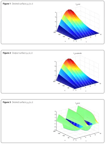
Figure 1Desired surfaceyd1(x,s)
Figure 2Output surfaceyk1(x,s)
Figure 3Desired surfaceyd2(x,s)
The desired trajectory is
Yd(x,s) =
Yd1(x,s),Yd2(x,s)
=
0.02ssin
x 11π
, 2cos
(10 –x)
2 π
1 –e–0.012xs.
FromGˆ(s) = I – G(s)(s), we can easily calculateρ< 0.5 and find it meets the conditions of Theorem1.
Figures1and3are the desired surfaces, Figs.2and4are output surfaces of the 20th it-eration. Figures5and6are the corresponding error surface of the 20th iteration. Figure9
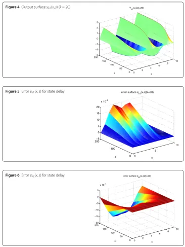
iter-Figure 4Output surfaceyk2(x,s) (k= 20)
Figure 5Errorek1(x,s) for state delay
Figure 6Errorek2(x,s) for state delay
ation errors are 2.0615×10–7,1.9855×10–6, respectively. Therefore, the iterative learning
algorithm (7) is effective for system (1a)–(1b).
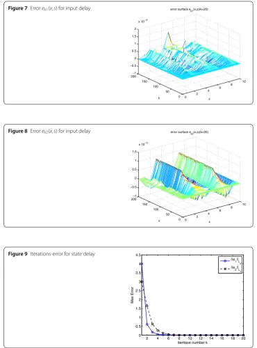
Secondly, we consider systems described by (2a)–(2b) with input time delay. Let
Bτ=
0.2 0 0.1 0.15
, C=
0.3 –0.1 0.1 0.4
, τ =
1 + 0.4e–5s 0.01 0 1.15 + 0.1e–4s
,
and select time delayτ = 8, Gτ = G, the rest are the same as those in system (1a)–(1b).
Figure 7Errorek1(x,s) for input delay
Figure 8Errorek2(x,s) for input delay
Figure 9Iterations-error for state delay
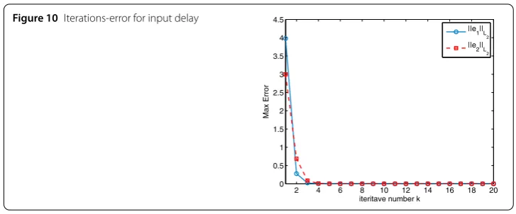
10denote that the tracking errors are already acceptable at the 10th iteration. The two error curves in Figs.9and10also demonstrate the efficacy of the proposed algorithms (7) and (48).
5 Conclusions
Figure 10 Iterations-error for input delay
Funding
The authors gratefully acknowledge the financial support of the National Natural Science Foundation of China (Grant Nos. 61863004, 61364006, 61563005), the Natural Science Foundation of Guangxi (Grant No. 2017GXNSFAA198179), and the Key Laboratory of Industrial Process Intelligent Control Technology of Guangxi Higher Education Institutes Director Foundation (No. IPICT-2016-02).
Competing interests
The authors declare that they have no competing interests.
Authors’ contributions
This work was carried out in collaboration among all authors. XD raised these interesting problems in this research. XM ([email protected]), YZ ([email protected]), and GX ([email protected]) proved the theorems, interpreted the results, and wrote the article. The numerical example is given by XY ([email protected]). All authors defined the research theme, read, and approved the manuscript.
Author details
1School of Electrical and Information Engineering, Guangxi University of Science and Technology, Liuzhou, China. 2Department of Mathematics, University of Kansas, Lawrence, USA.3College of Mathematics and Systems Science,
Shangdong University of Science and Technology, Qingdao, China.
Publisher’s Note
Springer Nature remains neutral with regard to jurisdictional claims in published maps and institutional affiliations.
Received: 10 July 2018 Accepted: 10 September 2018
References
1. Roesser, R.P.: A discrete state-space model for linear image processing. IEEE Trans. Autom. Control20(1), 1–10 (1975) 2. Cheng, S.S.: Partial Difference Equations. Advances in Discrete Mathematics and Applications, vol. 3. Taylor Francis,
London (2003)
3. Cheng, S.S.: Sturmian theorems for hyperbolic partial difference equations. J. Differ. Equ. Appl.2(4), 375–387 (1996) 4. Wong, P.J.Y., Agarwal, R.P.: Nonexistence of unbounded nonoscillatory solutions of partial difference equations.
J. Math. Anal. Appl.214(2), 503–523 (1997)
5. Xie, S.L., Cheng, S.S.: Stability criteria for parabolic type partial difference equations. J. Comput. Appl. Math.75(1), 57–66 (1996)
6. Zhang, B.G., Tian, C.J.: Oscillation criteria of a class of partial difference equation with delays. Comput. Math. Appl. 48(1), 291–303 (2004)
7. Liu, S.T., Guan, X.P., Jun, Y.: Nonexistence of positive solutions of a class of nonlinear delay partial difference equations. J. Math. Anal. Appl.234(2), 361–371 (1999)
8. Arimoto, S., Kawamura, S., Miyazaki, F.: Bettering operation of robots by learning. J. Robot. Syst.1(2), 123–140 (1984) 9. Sun, M.X., Wang, D.W.: Iterative learning control design for uncertain dynamic systems with delayed states. Dyn.
Control10(4), 341–357 (2000)
10. Sun, M.X., Wang, D.W.: Initial condition issues on iterative learning control for nonlinear systems with time delay. Int. J. Syst. Sci.32(11), 1365–1375 (2001)
11. Zhu, Q., Hu, G.-D., Liu, W.-Q.: Iterative learning control design method for linear discrete-time uncertain systems with iteratively periodic factors. IET Control Theory Appl.9(15), 2305–2311 (2015)
12. Li, X.-D., Chow, T.W.S., Ho, J.K.L.: 2D system theory based iterative learning control for linear continuous systems with time delays. IEEE Trans. Circuits Syst. I, Regul. Pap.52(7), 1421–1430 (2005)
13. He, W., Meng, T.T., Huang, D.Q., Li, X.F.: Adaptive boundary iterative learning control for an Euler–Bernoulli beam system with input constrain. IEEE Trans. Neural Netw. Learn. Syst.29(5), 1539–1549 (2018)
14. Dai, X.S., Xu, C., Tian, S.P., Li, Z.L.: Iterative learning control for MIMO second-order hyperbolic distributed parameter systems with uncertainties. Adv. Differ. Equ.2016(1), 94 (2016)
16. Shen, D., Xu, J.-X.: A novel Markov chain based ILC analysis for linear stochastic systems under general data dropouts environments. IEEE Trans. Autom. Control62(11), 5850–5857 (2018)
17. Li, Y., Jiang, W.: Fractional order nonlinear systems with delay in iterative learning control. Appl. Math. Comput. 257(15), 546–552 (2015)
18. Dai, X., Mei, S., Tian, S.: D-type iterative learning control for a class of parabolic partial difference systems. Trans. Inst. Meas. Control40(10), 3105–3114 (2018)
19. Dai, X., Tian, S., Guo, Y.: Iterative learning control for discrete parabolic distributed parameter systems. Int. J. Autom. Comput.12(3), 316–322 (2015)
20. Liang, C., Wang, J., Feckan, M.: A study on ILC for linear discrete systems with single delay. J. Differ. Equ. Appl.24(3), 358–374 (2018).https://doi.org/10.1080/10236198.2017.140922
21. Meng, D.Y., Jia, Y.M., Du, J.P., Yu, F.: Robust iterative learning control design for uncertain time-delay systems based on a performance index. IET Control Theory Appl.4(5), 759–772 (2010)