R E S E A R C H
Open Access
Utility-based efficient dynamic distributed
resource allocation in buffer-aided
relay-assisted OFDMA networks
Javad Hajipour
1*, Amr Mohamed
2and Victor C. M. Leung
1Abstract
In this paper, we study resource allocation in buffer-aided relay-assisted OFDMA networks. We consider utility-based stochastic optimization framework where there are constraints to be met either instantaneously or in average sense. Using the well-known Lyapunov drift-plus-penalty policy, we extract the instantaneous problem that needs to be solved in each slot to control the data admission and allocate the time slots, power, and subchannels. We propose the parameters that should be taken into account in utilizing the drift-plus-penalty policy in relay-assisted cellular
networks, for providing fair data admission and satisfying the average power constraints. We introduce a
low-complexity strategy for power and subchannel allocation and propose distributed and centralized algorithms to utilize it. Specifically, the proposed efficient dynamic distributed resource allocation (EDDRA) scheme is suitable for use in practice as it imposes less overhead on the system and splits the resource allocation tasks among the base station (BS) and the relays. Extensive simulation results show the effectiveness of the proposed parameters in meeting the objective and the constraints of the studied problem. We also show that the proposed EDDRA scheme has close performance to the proposed centralized one and outperforms an existing centralized scheme.
Keywords: OFDMA, Regenerative buffering relays, Distributed resource allocation, Low complexity
1 Introduction
Relay-assisted orthogonal frequency division multiple access (OFDMA) networks are the promising solutions for providing high-speed data services in wide cover-age areas and therefore, they have been accepted in the standardization bodies such as IEEE 802.16 [1] and long term evolution-advanced (LTE-A) [2] for providing wire-less access to the customers. Resource allocation is an important factor in utilizing the capacities of these net-works; while the combination of OFDMA and relaying techniques results in high benefits and opportunities, it also brings challenges and issues that need to be addressed for exploiting those opportunities [3]. There have been extensive works in this area in the recent years. In [4], the authors aimed at utilizing cross layer optimization frame-work for resource allocation in cooperative decode-and-forward (DF) relaying networks. For that, they introduced
*Correspondence: [email protected]
1ECE Department, The University of British Columbia, Vancouver, Canada Full list of author information is available at the end of the article
virtual links and nodes to embed the cooperation mech-anism into the optimization framework. They assumed half-duplex relaying and also considered spatial reuse of the spectrum among the links with lower mutual inter-ference on each other. Using dual method, then, they maximized the balanced end-to-end throughput. On the other hand, [5] considered reusing the OFDMA resources only among the different access links (from the relays to their users) and also suggested adaptive segmentation of the frame for transmissions on the base station (BS)-to-relay links and (BS)-to-relay-to-user links. To optimize these, the authors proposed linear-programming-based and greedy algorithms which led to significant improvements in the system capacity. However, the proposed algorithms in [4, 5] were centralized which impose high computational burden on the BS and high signaling overhead for report-ing channel state information (CSI) of the links. To alle-viate these drawbacks, several other works have studied distributed resource allocation [6–9]. In [6], cross layer scheduling in an OFDMA amplify-and-forward (AF) relay
network was studied to maximize the received goodput for the relayed users, taking into account the effects of imperfect CSI at the transmitter. Based on dual decom-position, a distributed algorithm was proposed for power and subcarrier allocation. Similarly, [7] proposed a dis-tributed algorithm for power and subchannel allocation based on dual decomposition, with the difference that the authors studied multiple-input multiple-output (MIMO) transmissions in a system with the possibility to dynam-ically select full-duplex or half-duplex, and AF or DF relaying. Pan et al. [8] investigated distributed power allo-cation algorithms in the presence ofcognitiverelays, based on convex optimization. They considered the cases with and without fairness considerations, with and without low signal-to-noise ratio (SNR) limitation on the BS-to-relay links, assuming fixed subcarrier allocations. More-over, they proposed a distributed scheme for joint power and subcarrier allocation. In contrast with the above works, [9] proposed a low-complexity semi-distributed algorithm for power and subcarrier allocation, by con-sidering complete/limited information about the CSI of the relay-to-user links at the relays/BS and assigning the subcarriers based on them. More other works studied fre-quency reuse schemes to improve the system capacity [10–12].
The common assumption in most of the literature in this area is that the relays do not have buffer to store packets for later transmission. Therefore, they have to forward their received data immediately in the following transmission interval. Recently it has been shown that the use of buffers in relays can improve the system capacity [13–15]. This is achieved as a result of more flexibility in transmissions from relays. In other words, buffering capability in relays enables them to postpone the data forwarding for a user if its channel is not good and use the wireless resources for the links with higher quality of channel.
Even though using buffers helps in compensating for the effect of channels in wireless networks, it also brings new challenges. In general, for better utilization of buffers, it is needed to take into account the queue dynamics in them. In this regard, different problems arising in different parts of these networks have been addressed in the literature. Yang et al. [16] studied adaptive media playout for video streaming, taking into account the queue dynamics in the receiver. By monitoring the queue size and its variation, a model was developed for buffer underflow probability estimation which was exploited to smoothly control frame separations of video traffic. In [17], a novel framework was proposed for online source rate control, where a buffer overflow probability (BOP) estimator monitors the queue sizes and its variation at the BS, and sends feedback about the estimated BOP to the video source to control its bit rate.
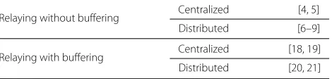
With the introduction of buffers in relays, several works also studied the challenges that arise for resource allo-cation in these networks. In [18], the authors studied resource allocation in a system with quasi full-duplex (quasi-FD) relays, where each relay is able to simultane-ously receive and transmit on orthogonal channels. They considered symmetric traffic for the users and proposed centralized algorithms for joint routing and subchannel allocation, to provide load balance among the cell nodes and fairness among the users. Compared with that, [19] studied a system with half-duplex (HD) relays where each relay can only receive in the first half of the frame and transmit in the second half. Then, using queue-length coupling across subframes, the authors proposed cen-tralized joint routing and subchannel allocation for each subframe and studied the system’s performance under both symmetric and asymmetric data traffic. In [20], the authors considered quasi-FD relaying and formulated a convex optimization problem for joint power and sub-channel allocation. Assuming a single power constraint for the whole system, a distributed resource allocation framework was proposed based on dual decomposition. On the contrary, [21] considered HD relays with individ-ual peak and average power constraints for the BS and relays, and studied joint optimization for subframe, sub-channel, and power allocation in LTE-A systems, where each subframe can either be used for transmissions on the BS-to-relays and BS-to-users links or the BS-to-users and relays-to-users links. Using utility-based stochastic network optimization [22, Chapter 5], and dual decompo-sition, optimal solution was provided for data admission into the network, and an iterative distributed algorithm was proposed for reaching the optimal resource alloca-tion. In Table 1, we have classified the most relevant references cited above, based on the usage of buffer and centralized or distributed approach of resource allocation algorithms.
The work in [21] is a pioneer in utilizing the Lya-punov drift-plus-penalty framework [22, Chapter 5] for data admission and resource allocation in OFDMA relay networks. However, it does not take into account some constraints and challenges that arise in practice in such networks. In particular, the proposed iterative algorithm to get the optimal solution incurs very low convergence rate due to the separate power constraints for the BS
Table 1Classification of the most relevant resource allocation references
Relaying without buffering Centralized [4, 5] Distributed [6–9]
and relays. This is not suitable for the practical sce-narios where the scheduling is performed in the units of millisecond. Also, it does not take into account the constraint that might be imposed on the buffer capac-ity in relays. Other than that, in the drift-plus-penalty framework, the average of a variable is defined over infinite time horizon, which requires some considera-tions for achieving the desired objectives and satisfy-ing the constraints in practical systems. To the best of our knowledge, none of the existing works on OFDMA relay networks has studied resource allocation with the abovementioned constraints altogether. This paper aims at addressing these issues and filling the gaps highlighted above.
In summary, we study low-complexity utility-based resource allocation in buffer-aided relay-assisted OFDMA networks, with HD relays, based on stochastic optimiza-tion framework presented in [22, Chapter 5]. We consider the network utility as a function of average data admis-sion of the users and aim at maximizing it subject to the long term and instantaneous constraints. Note that in our previous work [20], data admission was not stud-ied. Also, the resource allocation problem only had a single power constraint for the whole system, and there was no constraint on the transmission rates of the sub-channels (like finite data availability and limited buffer capacity). Therefore, it was possible to convert it to a convex optimization problem and use dual decompo-sition for power and subchannel allocation. However, in the current work, we consider several practical con-straints which necessitate a new solution approach. In addition to those constraints, the contributions of our current paper can be classified into two categories: one category is the identification of important factors that should be taken into account in the instantaneous prob-lem formulation. The other one is the design of low-complexity algorithms for solving the resource allocation subproblem. Specifically, the main contributions are as follows:
• We identify the factors that need to be taken into account for adapting the Lyapunov drift-plus-penalty policy for relay-based cellular networks. In particular, we propose to consider an importance parameter for average power constraint, to satisfy that constraint in a reasonable time period for practical scenarios. Also, we propose to add extra weight for the BS-to-relays and relays-to-users links, in the cases that the fairness is also an objective in the utility-based data admission control.
• We aim at low-complexity algorithms for time slot, subchannel, and power allocations and highlight the challenges even in such algorithms due to the lack of a priori knowledge about the subchannel sets and
total power usage of the BS and relays in each time slot. Then, we propose a low-complexity strategy for breaking the ties and making the correlations tractable, which can be used in both centralized and distributed resource allocation implementations.
• We focus on distributed mechanism for resource allocation and propose low-complexity algorithms for deciding about the type of time slot, subchannel sets of the nodes, and subchannel and power allocations to the links of the nodes. Based on that, we also present a low-complexity centralized mechanism which needs more signaling overhead and can be used as a baseline.
• We take into account practical constraints such as HD relaying operation, average and peak power constraint for each of the BS and relays, as well as limits on data availability and buffer capacity.
• Using extensive simulations, we demonstrate the effectiveness of the introduced parameters and also evaluate the performance of the proposed algorithms. We observe that the distributed scheme has very close performance to the centralized one and
outperforms an existing centralized scheme proposed in [19]. Also, we show that our proposed algorithms have similar or even better performance compared with the iterative algorithm proposed in [21] for reaching the optimal solution.
The rest of the paper is organized as follows. Section 2 describes the system model and the stochastic problem formulations. In Section 3, we state the subproblems and challenges as well as the proposed parameters and algo-rithms. Numerical results are provided in Section 4, with the conclusion finally presented in Section 5.
2 Preliminaries
In this section, we present the system model and the stochastic problem formulation. Then, we present the transformed version of the problem and introduce the virtual queues which make it possible to exploit the Lya-punov drift-plus-penalty policy in the next section. Here-after, for easiness, we will use the term “drift-plus-penalty” instead of “Lyapunov drift-plus-penalty”.
2.1 System model
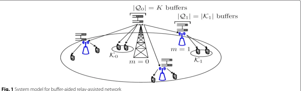
Fig. 1System model for buffer-aided relay-assisted network
byk ∈ K = {1,. . .,K},m ∈ M = {1,. . .,M} andn ∈ N = {1,. . .,N}. Table 2 presents the key notations used throughout this paper. We use the term “serving node” or simply “node” to refer to any of the BS or relays and show the set of all nodes byB = {0, 1,. . .,M}, wherem = 0 indicates the BS. Also, we useKmto denote the set of users that have a direct link to nodem∈B. On the other hand, m(k)is used to refer to the node directly serving userk.
We assume that time is divided into the units of slot, where each time slot can be either type A or type B. In type A slots, the BS transmits to users directly connected to it, or to the relays; in type B slots, the BS and relays can transmit only to the users connected to them and there-fore, there is no transmission from the BS to relays. This transmission format is based on LTE-A with type 1 relays where the BS-to-relays transmissions and relays-to-users transmissions use the same bandwidth but over different time slots, to prevent the interference between transmit and receive antennas.
We assume that the MAC layers of the BS and relays are equipped with buffers, where the BS has one for each user but every relay has one for each of the users con-nected to it. We denote the set of the users that have a buffer in nodem∈BbyQm; therefore, we haveQ0=K andQm = Km,∀m∈ M. These notations are defined to make the formulations and algorithms shorter. The data admitted into a BS buffer are queued until transmission to the corresponding direct user, or to the corresponding buffer in the relay serving the user. Similarly, data arrived at the relays’ buffers are queued until transmission to their users.
Note that in the following, when we use the term “the link of userkfrom nodem”, we mean “the link that serves the queue of user kin nodem”, which might be adirect link between the BS and a user, afeederlink between the BS and a relay or anaccesslink between a relay and a user connected to it. We useemkn(t)for the link of userkfrom nodemto denote the channel gain-to-noise ratio at the receiver side on subchannelnin time slott. It is assumed
that the channel conditions of the links vary over time and frequency, but remain constant during one time slot and over one subchannel. In the following, when we remove the (t) argument from the variables, we imply them in a general transmission incident. We assume that the BS and relays use M-ary QAM modulation for their transmis-sions; therefore, the achievable transmission rate on the link of userkfrom nodemon subchannelnin time slott can be computed as follows [23]:
rknm(t)=Blog2
1+ p m
n(t)emkn(t) k
, (1)
whereBis the bandwidth of a subchannel.k is the SNR gap due to the limited number of coding and modula-tion schemes and is related to the bit error rate of user k (BERk), through equationk = −ln(51.5BERk) [23].pmn(t) denotes the power allocated by nodemon subchanneln in time slott. We indicate the total power used by node m in time slott asPm(t) = Nn=1pmn(t). Using (1), the total transmission rate on the link of user k from node m can be written as rmk(t) = Nn=1xmkn(t)rknm(t), where xmkn(t)∈ {0, 1}denotes the subchannel allocation indicator which will be one if subchannelnis used for transmission on the link of userkfrom nodemin time slott, and zero otherwise. Note that for any n, in type A time slot, xmkn should be set to zero form ∈ M,k ∈ Km and in type B time slot,x0knshould be set to zero fork∈K−K0.
In each time slot, a resource allocation policy deter-mines the type of time slot, subchannel, and power allo-cations for the different links of the system. Based on that, the BS and relays transmit data from their queues, and at the end, the queue sizes are updated as follows:
Qmk(t+1)=minLmk, maxQmk(t)−Trmk(t), 0+amk(t), ∀m∈B,k∈Qm
Table 2Notation Summary
Notation Description
N,N Set and total number of subchannels, respectively M,M Set and total number of relays, respectively K,K Set and total number of users, respectively
B Set of all the serving nodes, including the BS and relays Km Set of users connected to nodem
Qm Set of users that have a buffer in nodem m(k) Serving node of userk
T Duration of a time slot
B Bandwidth of a subchannel
k SNR gap for userk
emkn(t),xknm(t) Channel gain-to-noise ratio and subchannel allocationindicator of subchannelnin time slott, respectively, for the
link of userkfrom nodem
rknm(t),˜rknm(t) Achievable transmission rate and estimated achievabletransmission rate on subchannel n in time slot t,
respectively, for the link of userkfrom nodem
rm
k(t) Total transmission rate on the link of userkfrom nodem in time slott
pm
n(t) Power used by nodemon subchannelnin time slott
Pm(t),Pˆm,Pavm
Total power to be used in time slot t, peak power constraint and average power constraint, respectively, for nodem
Lm
k,Qmk(t) Capacity of MAC layer buffer of userkin nodemand the queue size in it in time slott, respectively
amk(t) Size of data arrived at the MAC layer buffer of userkin nodemin time slott
ˆ
a Upper bound of data admission into a buffer in the MAC layer of the BS
Jk,Yk(t),Ak(t) Capacity, queue size and the arrived data size in time slot t, respectively, in the top layer buffer of userkin the BS U(.),V Utility function and the value coefficient for it, respectively
γk(t),Gk(t) Auxiliary variable corresponding to data admission of user kand its corresponding virtual queue size, respectively, in time slott
Zm(t),I Virtual power queue size of nodemin time slottand the importance factor, respectively, corresponding to average power constraints
ρm
k,We Indicator variable for the link of userkfrom nodemand the extra weight, respectively, for providing fair data admission
˜
Nm,Nˆm Estimation of nodemfor its number of subchannels and the upper bound considered by the BS on the number of subchannels for nodem, respectively
Dm
n,Dm Average demand of relaymon subchannelnand average total demand of nodem, respectively
D0a
n,D0a Average demand of the BS on subchannelnand average total demand of the BS, respectively, for type A time slot
D0bn,D0b Average demand of the BS on subchannelnand average total demand of the BS, respectively, for type B time slot
DA,DB Total demand for type A and type B time slots, respectively
whereT is time slot duration, andLmk andQmk(t), respec-tively, denote the buffer capacity of user k in node m and the size of data queued in it in time slot t. Data arrival process amk(t) into a relay buffer is in fact the departure process from the BS, and therefore, we have amk(t) = minQ0k(t),Trk0(t),∀m ∈ M,k ∈ Km. On the other hand, the arrival processes in the BS buffers are managed through a data admission control policy in the MAC layer, which decides to admit data or not to admit from the queues of the top layer buffers in the BS; this will be clarified in Section 3.2 and through (10). The size of the queues in top layer are updated as follows:
whereJkandYk(t), respectively, denote the buffer capac-ity of userk in the top layer of the BS and the size of data queued in it in time slott. Ak(t) is the amount of data arrived in time slot t for user k, according to an exogenous stochastic process, which is assumed to be stationary and ergodic. We assume that due to the pro-cessing limitations, an upper bound of aˆ is imposed on the amount of data admitted into the MAC layer buffers, and therefore, we have a0k(t) ≤ ˆa,∀k,t. Note that in the above, no specific assumptions have been consid-ered for queueing mechanisms other than the ordinary first-in-first-out (FIFO) operation and the layer-based architecture of data management, which has been con-sidered in [24] and [21] as well. In this paper, for sim-plicity, we have only considered the top layer and MAC layer in the BS and the MAC layer in the relays. How-ever, the discussions can be easily extended to the cases where the queueing in different layers are also taken into account.
2.2 Stochastic problem formulation
We note that in a realistic scenario, the BS buffers are not infinitely backlogged and are fed by stochastic data arrivals. This makes it necessary to take into account the queue dynamics, in the design of resource alloca-tion algorithms, in addialloca-tion to the randomness caused by the wireless channels. Therefore, theaverage perfor-mance metrics become important for network opera-tors, and especially, the average throughput and average power constraints are the issues that need to be man-aged. In the following, we will explain these in more detail.
by addressing the following stochastic optimization problem:
max a0,x,p
K
k=0
Ua0k , (4a)
s.t. C1 :Pm≤Pavm, ∀m∈B, (4b)
C2 :rkm(t)T ≤Qmk(t), ∀m∈B,k∈Qm, (4c) C3 :rk0(t)T ≤(Lmk −Qmk(t)),∀m∈M,k∈Km, (4d) C4 :rknm(t)≤Bˆs, ∀m∈B,k∈Qm,∀n, (4e) C5 :a0k(t)≤minaˆ,Yk(t)
, ∀k∈K, (4f)
C6 :a0k(t)≤Lk0−Q0k(t) ∀k∈K, (4g) C7 :Pm(t)≤ ˆPm, ∀m∈B, (4h) C8 :
m∈B
k∈Qm
xmkn(t)≤1, ∀n∈N, (4i)
C9 :{xmkn(t)}comply to the transmission rules of
either type A or type B slot (4j)
where U(.) is the utility function andC1 is to limit the average power consumption of each node.C2 shows that a finite amount of data can be transmitted from each queue andC3 is to prevent the incidents of more transmissions to relay buffers than they can accommodate.C4 indicates the limit on the availability of modulation schemes, where ˆ
sis the spectral efficiency of the highest order modulation in the system; considering it helps in controlling the power allocation and preventing overflows from relays’ buffers (This will be explained clearly in Section 3).C5 andC6, respectively, show the limit on the data admission from the top layer buffers of the BS and the limit on the available buffer space in the MAC layer of the BS.C7 indicates the maximum instantaneous power,Pˆm, that nodemcan use for transmissions,C8 shows that each subchannel can be allocated to only one link, and C9 is to use the feasible values for subchannel allocation variables{xmkn}.
The utility function in (4a) makes it possible to control the data admission for the users based on the objective of the network operator. For example for maximizing the total throughput,U(z) = zcan be used or for providing proportional fairness, U(z) = log(z) can be considered [22, Chapter 5]. We assume that U(z) is a concave and continuous function ofz.
Note that the problem (4) has two types of constraints. While C1 needs to be satisfied in long term, C2− C9 state the constraints that must be met in each time slot. In particular,Pavm is different fromPˆm, as the former can be set to limit the power consumption costs or the circuit heating but the latter is imposed by the system hardware (such as power amplifiers’ linear operation characteristics or maximum available instantaneous power) and is larger thanPavm.
2.3 Transformed problem and virtual queues
We note that the objective in problem (4) is a function of time average of users’ data admission rate. In order to uti-lize the drift-plus-penalty policy, it is needed to have the objective function as a time average expression. Similar to [22, Chapter 5], we define auxiliary variables 0≤γk(t)≤
ˆ
a,k=1,. . .,K, corresponding to eachak0(t),k=1,. . .,K. Then, the problem (4) can be transformed into the follow-ing equivalent problem, in which the objective is the time average of a function:
max a0,x,p,γ
K
k=0
U(γk), (5a)
s.t.C1−C9, (5b)
C10 :γk ≤a0k,∀k∈K, (5c)
C11 : 0≤γk ≤ ˆa (5d)
We also define the virtual power queuesZm(t)and vir-tual auxiliary queuesGk(t), respectively, corresponding to the constraintsC1 andC10, with the following updating equations:
Zm(t+1)=max[Zm(t)+Pm(t)−Pmav, 0] , ∀m∈B (6a)
Gk(t+1)=max[Gk(t)+γk(t)−a0k(t), 0] , ∀k∈K (6b)
Based on the abovementioned, we are able now to define the instantaneous problem (with the objective and con-straints stated in terms of the instantaneous values of the variables) and study the algorithms for solving it, which will be presented in the next section.
3 Cross layer traffic control and resource allocation
3.1 Instantaneous problem
To address the problem (5), based on the drift-plus-penalty policy [22, Chapter 5], we define the “instanta-neous” problem in time slottas follows:
max
whereV > 0 is the value that can be given to the objec-tive (5a), and by that, we can trade off higher utility to larger queue sizes [22]. This will be clarified later. I > 0,ρkm ∈ {0, 1} andWe > 0 are the parameters that we propose in this paper, to adapt the drift-plus-penalty pol-icy to relay-assisted cellular networks.Iis the importance factor that we give to average power constraint, through which we can prevent the continuous growth of the virtual power queues and consequently, we can meet the average power constraints in shorter time.Weis an extra positive weight, that can be given to the feeder links from the BS to relays and the access links from relays to users, in the cases that the fair admission of users’ data is of our con-cern.ρkm is the indicator variable to specify the cases to applyWe; in particular, it is set to zero unless when the fair data admission is desired and the corresponding queue (either in the BS or in a relay) belongs to an indirect user, i.e.,k ∈ K−K0,m ∈ B. Proposition ofI,ρmk andWeis one of the main contributions of our paper and will be dis-cussed later. Based on the above, we can see that the work in [21] is in fact a special case of our work, in whichI=1, ρm
k =0,We=0 and no limitations on buffer capacities or modulation schemes are considered.
It is observed from (7a) that, using the drift-plus-penalty policy, the instantaneous objective in each time slot includes four terms: the first term corresponds to the long term objective (5a) and the rest correspond to serv-ing the actual queues and stabilizserv-ing the virtual queues (to meet the constraintsC1 andC10). We note that due to the limited buffer capacities, the actual queues of the system are always stable. However, using drift-plus-penalty policy provides a useful framework for channel- and queue-aware resource allocation which takes into account both the channel states and the data availability in the sys-tem’s actual queues. It also makes it possible to stabilize the virtual queues {Gk(t)} and {Zm(t)}. It is shown in [22, Chapter 5] that solving the instantaneous problem obtained from drift-plus-penalty policy in the case of infi-nite buffer capacities (i.e., when the constraintsC3 andC6
are not imposed) provides a utility (4a) that has a gap of D
V from its optimal value, whereDis a constant related to sum of the squared data arrivals and squared transmission rates. If the solution algorithm for instantaneous prob-lem (7) also leads to an approximate value of the objective function (7a) within distance C from its optimal value (e.g., due to a suboptimal solution), then the aforemen-tioned gap will beD+VC. Therefore, there is anO(1/V)gap between the optimal utility of the stochastic problem and the utility obtained from solving the instantaneous prob-lem, which can be arbitrarily reduced by choosing a large V. However, this will lead to larger queue sizes and delays due to the fact that the upper bound on the queue sizes has anO(V)expression. Recently, [25] has shown that in the case of finite buffer capacity ofβ, the utility obtained from drift-plus-penalty policy is withinO(1/V)+O(e−β)of its optimal value. Note that [25] assumes that each node is allowed to transmit to the next hop even if it does not have enough buffer space, in which case the received packet is dropped. However, this is not allowed in the system con-sidered in our paper, due to the constraintC3, as it will waste the (expensive) frequency resources. This makes the mathematical analysis of the drift-plus-penalty policy difficult in our system model and can be investigated in future works.
It is worth mentioning that considering V, I, ρkm, and We in (7a) facilitates reaching our goals for system util-ity and constraints in different scenarios; neglecting them is in fact like setting them based on a fixed scenario (i.e., V = I = 1 and We = 0) which would lower the use-fulness of the drift-plus-penalty policy. Note thatVandI can be tuned easily by considering the range of values for weighted rates in (7a), affected by packet sizes and trans-mission rates. On the other hand,ρkmcan be easily set as stated above, when fairness is an objective; then,Wecan be tuned by increasing its value from zero towards the val-ues in the range of queue sizes in relays, depending on how much we trade off between data admission for the direct and indirect users. These will get clearer in the next section, when we discuss their effects.
Similar to [22], by rearranging the terms in the instanta-neous problem, it can be divided into three instantainstanta-neous Subproblems (SPs) which will be presented in the next subsections.
3.2 Traffic control and data admission
The first subproblem of (7) is related to the auxiliary variables as follows:
SP1 (auxiliary variable subproblem) :
SP1 is a simple convex optimization problem and there-fore, the BS can solve it easily. As an example, for the proportional fairness, i.e., when U(γk) = log(γk), after taking the derivatives, the BS can determine the optimal auxiliary variables in time slottthroughγ1
k(t) =
Gk(t)
V =⇒
γk(t)= min
ˆ
a,GV
k(t)
,∀k. After computing the solution, the BS can update the corresponding virtual queue sizes based on (6b).
The second subproblem of (7) is related to the flow con-trol and data admission into the users’ buffers in the MAC layer of the BS, as follows:
SP2 (flow control subproblem) :
max a0
K
k=1
Gk(t)−Q0k(t)
a0k(t), (9a)
s.t. 0≤a0k(t)≤ ˆa,∀k∈K, (9b) a0k(t)≤minYk(t),L0k−Q0k(t)
,∀k∈K (9c)
which is a linear problem; by solving it, the BS can deter-mine the optimal data admissions in time slottas:
a0k(t)=
minYk(t), min
ˆ
a,L0k−Q0k(t),Q0k(t)≤Gk(t)
0 , otherwise
(10)
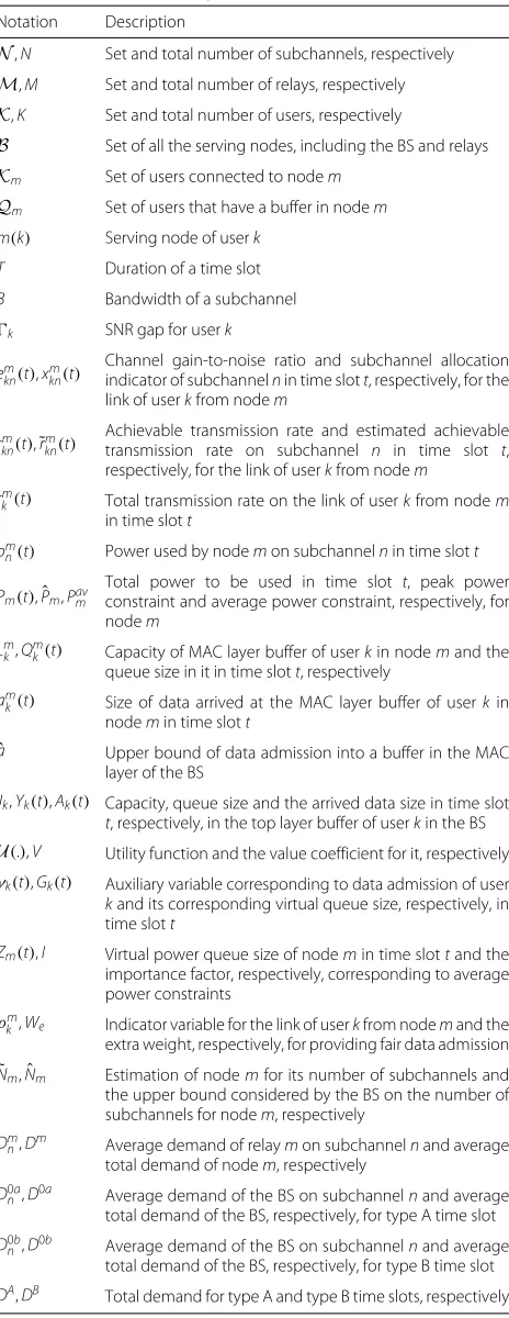
Based on the above, for deciding about data admis-sion for user k, the BS needs the information about its top layer queue sizeYk(t), MAC layer queue sizeQ0k(t), auxiliary variable’s virtual queue size Gk(t), maximum admissible data sizeaˆ, and the MAC layer’s buffer capac-ity L0k. All of these information are accessible to the BS as the related buffers and queues are implemented in the BS.aˆ andL0k are fixed parameters;Yk(t),Q0k(t) and Gk(t)are in fact the input variables to the data admission procedure in the MAC layer of the BS and the decision about the size of admitted data is the output. This is
clarified in Fig. 2. After determining data admissions and transmissions (discussed later), the BS can use (2) and (3) to update the affected queue sizes. It is worth mention-ing that the data admission procedure presented above is based on [22, Chapter 5], and its inclusion here is for completeness of the discussions presented later.
Note that based on (10), whenever the size of an actual queue at the BS, Q0k(t), is larger than the virtual queue Gk(t), no data is admitted into the corresponding BS buffer. This can happen for several time slots, in buffer-aided relay-assisted cellular networks, due to the admis-sion of a large packet and low service rate of the queue of an indirect user at the BS (which is caused by the differential backlog terms described in the next subsec-tion). Consequently, even using a utility function with fairness property and large value for parameterV does not necessarily lead to fair data admission, and therefore, more considerations are needed in resource allocation for serving the queues. This is the motivation for proposing ρm
k and the extra weight We (explained clearly later, in Remark 1), which help to improve the fair data admission for indirect users.
3.3 Resource allocation challenges
By substituting (1) in (7a) and removing the constant terms, the last and most important subproblem, which is to decide about the time slot, subchannel and power allocations, can be stated as
SP3 (resource allocation subproblem) :
max p,x
N
n=1 M
m=0 ⎛
⎝
k∈Qm
BTwmk(t)log2
1+ p m
n(t)emkn(t) k
−IZm(t)pmn(t) ⎞
⎠, (11a)
s.t.C2−C4,C7−C9 (11b)
wherew0k(t)= Qk0(t),k∈K0(weights for the direct links from the BS to its users; recall thatρk0is always equal to 0 for these links),wmk(t)=Qmk(t)+ρmkWe,m∈M,k∈Km (weights for the access links from relays to their users), andw0k(t) = Qk0(t)−Qkm(k)(t)+ρk0We,∀k ∈ Q0−K0 (weights for the feeder links of indirect users from the BS to relays). The differential backlog termQ0k(t)−Qmk(k)(t) in the weight of a feeder link is resulted by switching the sums and considering the fact that for the buffers of the relays, the arrivals are upper bounded by the transmis-sion rates from the BS to relays, i.e.,amk(t) ≤r0k(t),∀m∈ M,k∈Qm. As explained in the previous subsection, and later in Remark 1, these differential backlog terms lead to unfair data admission for indirect users, and their effect can be reduced by usingρkmWeterms.
We note that SP3 is a mixed integer and nonlinear programming and needs an exhaustive search to find its optimum solution. One common approach for these types of problems is to relax the subchannel allocation variables xmkn whenever this relaxation converts the problem into a convex one. Then, using the dual decomposition, opti-mal solution can be found, if the duality gap is zero. This approach was used in our previous work in [20], based on which we proposed a dynamic distributed resource allo-cation. However, in the current paper, due to the finite data and limited buffer capacity constraints, i.e.,C2 and C3, the resulted problem after relaxation ofxmkn variables will be non-convex. In addition, we note that in [20], there was only one power constraint for the whole system which made it possible to have high convergence speed for the proposed algorithm. In a more realistic system like the one we consider in the current paper, the BS and relays have separate power constraints. Therefore, even if we remove the constraintsC2,C3 and relaxxmkn variables to make it convex, a dual-based iterative algorithm will need many iterations and a long time to converge. This is not suit-able for use in practical scenarios where each time slot is in the order of a millisecond, and the resource allo-cation decision needs to be made in a small fraction of time.
Due to the abovementioned, we aim at low-complexity suboptimal algorithms which can be easily implemented in practical systems. For this purpose, we consider equal power allocation on subchannels and allocate them in a greedy way, based on the queue sizes and achievable trans-mission rates of the links. This is not only for making the resource allocation practical, but it is also reasonable, because when adaptive transmission rates are used (as in our system by (1)), optimal power allocation results in marginal gains [26].
However, even considering equal power distribution on subchannels and computing the achievable transmission rates of the links is not trivial here, due to the following two issues:
a) Unknown number of subchannels for each node. For deciding about the allocation of subchannels, we need to know the achievable transmission rates of the links on the subchannels, and for that we need to know the power allocations on the subchannels. However, before subchannel allocation, it is not clear how many subchannels will be allocated to the BS and relays, and consequently, it is not known on how many subchannels their total powers will be
distributed equally.
b) Unknown total powers to be used by each node. The total powers used by each of the BS and relays need to satisfy the average and peak power constraints. This is controlled in SP3 by constraintC7and the objective function which is the sum of increasing and decreasing functions of power. Based on that, the total power used by each node can vary in each time slot between zero and its peak value, depending on the subchannel allocations and the size of the corresponding virtual power queue. Therefore, even if we make an assumption on the number of subchannels to be used by each node, it is not clear that how much total power will be distributed equally on them.
To address the above issues, we propose a low-complexity suboptimal strategy, as shown in subchannel and power allocation strategy (SPAS), which breaks the interdependence between power allocation and subchan-nel assignment. At the beginning, SPAS assumes that
Subchannel and power allocation strategy (SPAS)
• Assume the number of subchannels that nodem will use for its transmissions,N˜m, will be proportional to
the number of its queues.
• Assume that each nodem will use its peak power (which will be equally distributed on its subchannels, i.e., it will use Pˆm
˜
Nm for transmission on each of its
subchannels).
• Estimate the achievable transmission rates of the links of the nodes based on their channel conditions and the abovementioned assumption for powers.
• Determine the type of time slot and allocate the subchannels to the system links, based on the estimated achievable transmission rates and actual queue sizes.
the number of subchannels that each node will use for its transmissions will be proportional to its number of queues, and the total power each node will distribute on its subchannels will be its peak power. Based on that, SPAS estimates the transmission rates of the links to be used in making a decision about the type of time slot and subchannel allocation. At the end, it adjusts the total pow-ers, considering the size of actual and virtual queues. The details for these are presented in the next subsections.
Note that SPAS in fact provides a plan which can be uti-lized for designing the resource allocation algorithms in a centralized or distributed way. In the following, we will present the distributed implementation, as it is of more interest to the research and industrial bodies; later, we will describe the centralized resource allocation which can be used as a baseline for the proposed distributed one.
3.4 Efficient dynamic distributed resource allocation In this subsection, we propose the EDDRA method which performs resource allocation in each time slot, through four steps. In the first step, every node reports estimates of its subchannel demands to the BS and based on them, the BS decides about the type of time slot. In the sec-ond step, the BS determines and reports the subchannel sets that each of the BS and relays can use. Then, in the third and fourth steps, in a distributed way, each node first assigns the subchannels to its users and then adjusts the total power it can distribute over its subchannels.
Step 1) Slot Type Determination (STD). At the end of each time slot, first, the BS needs to specify the type of the next slot. For this, relays report an estimate of their average demand for each subchannel to the BS. These demands are computed based on the assumptions on the number of subchannels they can get and the total power they can use. Then, the BS uses the reported demands from the relays as well as its own demands to estimate the system’s total demands for type A and type B slots, and based on that, it decides about the type of the next time slot. This is outlined in STD algorithm and the details are described in the following.
Based on SP3, we define the estimated average demand of nodem∈Mon subchannelnas
sion rate of the link of userkfrom nodemon subchannel n. It is computed in node m, m ∈ M, assuming that the number of subchannels it will get,N˜m, is proportional to the ratio of its number of queues (|Km|) and the total
number of queues that can be considered for service in type B slotm∈B|Km| =K ; i.e.,
˜
Nm=N|Km|
K ,∀m∈B, (13)
Since the BS knows the number of queues in each relay, it can easily estimate their total demands as in line 2 of STD algorithm. For itself, the BS needs to compute sepa-rate demands for type A and type B slots. Noting that in type B slots, it can only transmit to its direct users while sharing subchannels with relays, its average demands are computed similar to relays and based on the weights and rates of the links of direct users (assuming the transmis-sion power on each subchannel equal to Pˆ0
˜
Algorithm 1Slot Type Determination (STD)
1: Each relaym∈Mreports to the BS, its estimated average demands on all subchannels, i.e.,Dmn, ∀n∈N.
2: The BS estimates the total demand of each relaymas Dm= |Km|Nn=1Dmn,m∈M
3: The BS estimates its own demand for type A slot as
D0a=KN n=1D0na
4: The BS estimates its own demand for type B slot as
D0b= |K0|Nn=1D0nb
5: The BS estimates the total demand for type A slot as
DA=D0a, and for type B slot asDB=D0b
On the other hand, we note that in a type A slot, only the BS can transmit and all the queues in the BS (including those of indirect users) can be served using all the subchannels; thus, its total demand is computed based on the weights and rates of all of its links and assuming Pˆ0
relays is min(K − |K0|,N)). Therefore, in EDDRA, the total overhead of signaling about the demands and the modified queue sizes is ofO(min(K− |K0|,N)+MN).
Remark 1.Here, we explain the reason for usingρmkWe in the weights of the links of indirect users from the BS and relays. Without that, due to the low powers of relays and low transmission rates, their demands would not be comparable to the demands of the BS for direct users, unless the queues in relays grew large. On the other hand, for the links serving the queues of indirect users in the BS, we would havew0k = Q0k−Qkm(k),∀k ∈ K−K0. As a result, these would not have enough impact on comput-ing the average demands for indirect users and providcomput-ing service for them (in the cases that the queue sizes of an indirect user in the BS and relay have the same size, Q0k = Qmk(k), the impact would be zero). Consequently, the queues of indirect users in the BS would usually have larger sizes than the queues of direct users, and there-fore, data admission for them would be less. This would degrade the usefulness of drift-plus-penalty for cellular networks, because fairness is usually one of the main con-cerns in these networks. To prevent that, ρmk should be set to 1 for the feeder and access links andWeshould be applied as mentioned in subsection 3.1. This will compen-sate for the effect of low power of relays on the demands of access links and the effect of differential-backlog-based weights on the demands of feeder links. Similar effect holds also in the subchannel sets determination and subchannel allocation steps which will be described later.
Step 2) Subchannel Sets Determination (SSD). We note that in a type B slot, due to sharing subchannels among all the nodes, the resource allocation for the links of different nodes are tied together which is reflected in (11). In this step, the goal is to break this tie and specify the subchannel sets to be used for transmissions from the BS and relays. This allows to have the resource allocation in a distributed manner at each node.
For the above purpose, when the slot is decided to be type A, the BS notifies the relays about it and they know they have no transmissions. In the case of a type B slot, the BS determines the subchannel sets of the relays and noti-fies them to transmit on them. SSD algorithm shows the whole procedure in detail. Since in type B slots, the BS can only transmit to the direct users, line 5 of the algorithm defines its demands based on the estimations for type B slot, explained before. Line 6 setsNˆm, as the upper bound for the number of the subchannels that each node can get, and the next lines assign the subchannels to the nodes that have not reached their limit on the number of subchannels and have higher average demands on the subchannels.
Algorithm 2Subchannel Sets Determination (SSD)
1: ifthe slot type is A
2: The BS determines subchannel sets asN0=Nand Nm= ∅,m∈M
3: else
4: The BS specifies subchannel sets, based on the relays’
demands as well as its own, as follows
5: SetD0n=D0nb
17: The BS notifies relays about their subchannel sets
Note that setting the limitNˆm for the size of the sub-channel set of nodemis to prevent nodemfrom getting subchannels more than it needs. For example, a relay might have only one user with highaveragedemands on the subchannels while another relay with several users might have a little loweraveragedemands on the subchan-nels. In such a case, without considering the total number of users and the limit for subchannel set sizes, the relay with a single user would overshadow the other relay in all the iterations of subchannel assignments through line 9.
The computational complexity of the SSD algorithm is of O((M+1)N2), which is obtained by ignoring the insignificant computations and considering the number of iterations needed for performing line 9.
Step 3) Subchannel Allocation (SA). After determin-ing the subchannel sets, the resource allocation sub-problem (11) can be further decomposed into separate subsubproblems, as follows:
SSP(resource allocation subsubproblems) :
max
C7 − C8. For this purpose, following the SPAS strat-egy, we propose to have subchannel allocations by each node based on using Pˆm
|Nm| (i.e., assuming Zm(t) = 0)
for computing the achievable transmission rates. Then in the power adjustment step, considering the real value ofZm(t), each node can decide about the total power it should use and distribute it on its subchannels.
Algorithm 3Subchannel Allocation (SA) in the BS
1: if slot type is A, setQ =Q0, otherwise, setQ =K0
Noting that the BS has more constraints than the other nodes (the constraint C3 is only enforced on the feeder links from the BS, which is to prevent transmitting data to the relays more than their empty buffer spaces), we pro-vide the subchannel allocation by the BS and then explain its use for relays. SA algorithm shows the details in allo-cating the subchannels by the BS. The procedure is done in an iterative way with |N0| iterations. In each itera-tion, the weights of the links and the resulted demands are computed, and the pair of subchannel and queue with the highest corresponding demand is selected. Then, the selected subchannel is assigned to the link serving the selected queue and the size of the affected queues are updated virtually. Since the actual queue sizes, Qmk, are only updated at the end of transmission intervals, we have usedqmk variables to prevent ambiguity about the updating during the algorithm iterations. Note that these updates are done to meet the constraints C2 and C3. Line 6 is for applying the extra weightWe, described before. How-ever, before adding it, by comparing the queue size with BTˆs, we make sure that there are enough data such that
they can utilize the subchannel completely if it is allocated. Line 7 is to meet the constraintC3 and prevent overflow, by giving a negative weight in case the remaining empty space in a relay buffer is less than the possible maximum transmission size on a subchannel. If a feeder link gets negative weight, then it will not be considered for sub-channel allocation and this will prevent transmitting data to the corresponding relay buffer.
Remark 2. Note that the rate computations in SA are based on the assumption of equal distribution of peak powers on the subchannel sets. This way, we will be sure that when in Step 4, the total power is adjusted (which certainly will be equal or less than the peak power), the transmission rate for each link will be less than the amount considered in SA algorithm, and therefore, the constraints C2 andC3 will not be violated.
In type B time slots, in parallel to the BS, any relay also uses the SA algorithm with the difference that all the superscripts/subscript 0 are replaced by the correspond-ing m. Note that in this case we have Q = Km and Q −Km = ∅. Hence, the lines 5, 7, 12 are not executed when SA algorithm is used by relays. Based on the above-mentioned, the subchannel allocation task in EDDRA is split among the serving nodes, where the computational complexity of the SA algorithm in any nodem ∈ Bis of O(|Nm|2|Qm|).
Step 4) Total Power Adjustment (TPA). After assign-ing the subchannels to the links, the BS and relays decide about the total power that they can distribute on their sub-channels to meet the constraintsC4,C7. For this, based on SSP in (14), each nodemsolves the following problem, which we refer to as the total power adjustment, to find the total power,Pm, that it can use.
TPA(total power adjustment problems) :
max queue of which the subchannelnhas been allocated. The TPA problem is a convex problem with one variable. Thus, the optimal value,P∗m, can be found easily by using an iter-ative one-dimensional search such as the Golden Section method [27, Appendix C.3], which has the computational complexity ofO(log(1/1)), where1is the desired relative error bound.
defined for that purpose. In fact, based on (6a), having a nonzeroZmmeans that in the past time slots, there have been the events of transmission with the total power,Pm, larger than the average power limit,Pavm. Therefore, in TPA problem,Zm applies a kind of negative feedback to use less power thanPˆm. The proposed importance factorIis in fact for amplifying this negative feedback to adjust the total power use in a short period of time. Without it, the second term in the objective (15a) would not be compara-ble to the first one over a large period of time slots, before Zm becomes big enough to impact the objective value. This is due to the fact that the values of the power vari-ables are very small (in the order of 1–10 watts) compared to the values of queue sizes multiplied by transmission rates (in the order of tens of megabits).
After findingP∗m as described above, each node com-putes the power on its subchannels, considering equal power distribution and noting that the rate on each sub-channel can not be larger than Bsˆ (due to the limited spectral efficiency of modulation schemes in practice); i.e.,
pmn =min
P∗m
|Nm|,
(2ˆs−1)k(n) emk(n)n
,∀m∈B,n∈Nm
(16)
The reason for considering the term withˆsin (16) is to prevent using the power more than needed for maintain-ing the desired bit error rate. It is obtained based on (1) andC4.
After the above steps, based on the variablesxmknandpmn, each node notifies its users about the subchannel alloca-tions and the assigned transmission rates. Then, it trans-mits to them and updates its actual and virtual queues using (2) and (6).
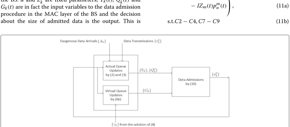
Remark 4.As discussed in subsection 3.3, the resource allocation subproblem (11) is not a convex optimiza-tion problem; therefore, the existence of global optimal is unknown. The algorithms proposed in the STD, SSD, SA, and TPA steps provide a suboptimal solution which have low overhead and low computational complexity, and, as shown in Section 4 (Figs. 5, 6, 7, 8, 9, and 10), lead to better performance compared with an existing suboptimal algo-rithm. Moreover, to the best of our knowledge, even when the constraintsC3 andC6 are not imposed (i.e., assum-ing infinite buffer capacities), there is not a clear method to compute mathematically the distance of our proposed scheme from the optimal solution of the corresponding convex optimization problem, as it is heuristic. However, as shown in Section 4 (Figs. 13, 14, 15, and 16), depend-ing on the value ofVin this case, our proposed algorithms can lead to higher or slightly lower system utility (at the cost of higher queue sizes) compared with an existing
algorithm which uses subgradient method to reach the optimal solution.
Remark 5.Note that the Steps 1 to 4 are executed only once in each time slot. Also, STD, SSD, and SA algorithms have a fixed number of iterations/operations after which they terminate, and there is no need to analyze their con-vergence. On the other hand, as stated in Step 4, TPA problem is a single-variable convex optimization problem and therefore, any one-dimensional search is guaranteed to terminate when reaching the specified tolerance of1.
3.5 Efficient dynamic centralized resource allocation (EDCRA)
In this subsection, we briefly describe the EDCRA method, in which the BS performs all the procedures for resource allocation. In a centralized scheme, the BS needs to get notified about the channel states of all the links in the system over all the subchannels1. For this purpose, since the indirect users do not have connection to the BS, the relays report to the BS about the channel conditions of the access links (which already have been reported by the indirect users to their serving relays). This imposes a sig-naling overhead ofO((K− |K0|)N)from relays to the BS. Considering the fact that in practice the number of users is remarkably more than the number of the relays, the sig-naling overhead in EDCRA is a lot more compared with EDDRA2(which is ofO(min(K− |K0|,N)+MN)).
Having all the information about the channel states and the queue sizes, the BS performs STD procedure and if the slot type is set to A, it uses the SA algorithm as in EDDRA. However, if the slot type is set to B, the BS does not need to run SSD algorithm. Instead, considering the set of all the subchannels, it uses SA algorithm as fol-lows. The queues in relays are assumed to be located in the BS, and their corresponding access links are assumed as direct links starting from the BS to the indirect users; however, the weights and channel rates are considered the same as those of actual access links. Then, SA algorithm is exploited to decide about the subchannel allocation to the different links in the system, which incurs the compu-tational complexity ofON2m∈B|Km| = O(N2K). After that, based on the corresponding subchannel allo-cations for all the nodes, i.e.,{xmkn}, the BS specifies the powers to be used by each node by performing the total power adjustments for them. Finally, the BS informs all the relays about the subchannels and powers they can use.
for future works to design data admission and resource allocation algorithms in the presence of the services with strict QoS requirements.
4 Performance evaluation and discussion
To evaluate the performance of the proposed algorithms, we have conducted extensive simulations for a system with M=6 relays, which are located in the distance of 2/3 of the cell radius from the BS and in an equal angular dis-tance from each other. The simulation parameters are as in Table 3, unless otherwise specified. For the links from the BS to relays, channels are assumed line-of-sight (LOS)-based and therefore, Rician channel model, withκ factor equal to 6 dB, is considered; for the links between the BS/relays and users, channels are assumed non-LOS (NLOS)-based and therefore, Rayleigh channel model is used [28]. For computing the path loss of the links, we have considered the COST231 Hata urban propagation model which uses the following equation [29]:
PL=(44.9−6.55 log10(htx))log10
d 1000
+45.5
+(35.46−1.1hrx)log10(fc)−13.82 log10(htx) +0.7hrx+3,
(17)
where PL is the path loss in dB, htx is the transmit-ter antenna height in metransmit-ters,hrx is the receiver antenna height in meters,fcis the carrier frequency in MHz, and d is the distance between the transmitter and receiver in meters. The above model for path loss has been con-sidered in [29] for urban Macrocell environment, where the distance between the BS of the adjacent cells is larger than 1 km. Due to the fact that using relays in cellular networks makes it possible to have a large coverage area for a single cell, served through the BS and relays, we
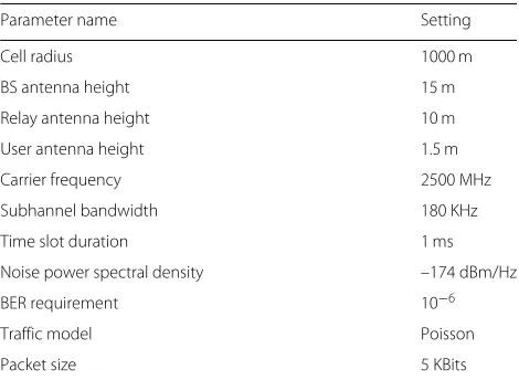
Table 3Simulation parameters
Parameter name Setting
Cell radius 1000 m
BS antenna height 15 m
Relay antenna height 10 m
User antenna height 1.5 m
Carrier frequency 2500 MHz
Subhannel bandwidth 180 KHz
Time slot duration 1 ms
Noise power spectral density –174 dBm/Hz
BER requirement 10−6
Traffic model Poisson
Packet size 5 KBits
have assumed the network environment as urban macro-cell and have used the above equation. We acknowledge the fact that, in reality, the channel behaviors in cellular networks might be different from the models considered in our simulations. However, considering the fact that the same models have been used in simulating the behav-ior of the baseline algorithms existing in the literature, the relative performance improvements of our proposed algorithms, presented later, are expected to hold.
For utility function, we have consideredU(z) = log(z) to provide proportional fairness. Due to the large packet sizes which resulted in large queue sizes, based on the observations from simulation results, we have chosenVto be 107. This gives high value for utility function in (7a) to be comparable to the terms related to the weighted trans-mission rates. The buffer capacities at the BS and relays are considered equal to 100 and 10 packet sizes, respec-tively. The highest order for modulation is assumed to be 64 QAM which has the spectral efficiency of 6 bits/sec/Hz. In the following, we first consider a special scenario with the settings as follows. The data arrival rate of each user is 100 packets per second, or equivalently 500 kbps. The peak power of the BS is equal toPˆ0 = 34 dBm and the peak power of the relays are equal to Pˆm = 25 dBm, m ∈ M. The average power constraint of the nodes are half of their peak power constraints, i.e., 31 dBm= 1259 mW for BS and 22 dBm= 158 mW for relays. The num-ber of subchannels is considered equal toN = 7. There are 12 users in the system, 6 of them connected directly to the BS and the rest connected to relays, one user per relay. The distances of the direct users from the BS and the indi-rect users from the corresponding relays are 300 m. Note that this special scenario, with the mentioned settings, is to provide an example to show the necessity of consid-ering the importance parameterI in practical scenarios. The values of the different parameters are selected specif-ically for simulation purpose. However, in practice, these values are possible. For instance, the indirect users’ loca-tion are considered 300 m from relays to simulate the case that those users are close to the cell edge, and the direct users location is selected 300 m from the BS to simulate an average location between the BS and relays. On the other hand, the number of subchannels is selected equal to seven to have, on average, one subchannel for each of the serving nodes (the BS and six relays). Even though seven subchannels might not correspond to an explicit standard bandwidth, it can happen in practical systems. For exam-ple, the operators might allocate the system resources separately for different classes of users and reserve spe-cific number of subchannels for each class of users, using the number of serving nodes as a rule of thumb.
Fig. 3Effect of parameterIon average power consumption of the BS and relays;N=7,|K0| =6,|Km| =1,m∈M
size corresponding to the average power constraint of the BS during the mentioned period. It is observed that with-out considering a suitableI(e.g., whenI= 1 orI= 103), the average power consumption of the BS is about 2000 mW, which is far beyond the constraint of 1259 mW, and the size of virtual power queue of the BS grows constantly over this period. This happens due to the fact that in (15a),
the value of the second term is very small compared with the value of the first one and as a result, it does not have much effect on the optimization objective; therefore, the only thing that limits the total power usage is the peak power or the maximum spectral efficiency. The conse-quence of this is the steady use of the peak power of the BS in each time slot, which incurs the steady growth of its virtual power queue size according to (6a). Without a suit-ableI, this would continue for a long time, until the size of the virtual queue has grown so large that the second term in (15a) is comparable to the first one. However, as stated in Remark 3, using a suitably largeI(e.g.,I = 106in this scenario) amplifies the effect of the virtual power queue sizes in (15a) and prevents continuous use of the peak powers. Therefore, as shown in Fig. 4, the virtual power queue of the BS gets bounded after about 300 time slots and, as displayed in Fig. 3, the average power consumption of the BS over the simulation period is about the speci-fied constraint. It is worth mentioning that due to fewer transmissions from the relays, compared with the BS, their virtual power queues did not grow large and remained sta-ble in all the above values forI and had similar graphs as that of the BS in the case ofI = 106. Because of this similarity, their graphs were omitted.
To investigate the overall performance of the proposed algorithms in general scenarios, we consider a system with 25 users, which are uniformly distributed in the cell area and are connected to the node from which they receive higher signal strength. The simulations are conducted for
100 runs, each over 10,000 time slots, to generate differ-ent realizations of users’ locations. All the users have the data arrival rate of 20 packets per second or equivalently 100 kbps, and the buffer capacity in the BS and relays are, respectively, 100 and 10 packets per user. There are 14 subchannels in the system, the BS’s peak power is 37 dBm, relays’ peak powers are 28 dBm, and the average power constraints are half of the peak powers. As a baseline, we have adapted the low-complexity centralized algorithm proposed in [19] to our system model, which we refer to as fixed half-duplex relaying (FHDR) in the figures. With FHDR, the type of the time slots are fixed such that the odd-numbered time slots are used for the transmissions from the BS and the even-numbered slots for the trans-missions only from the relays. The subchannel allocations in even-numbered slots are based on considering a mini-mum ofN/Msubchannels for each relay and assigning them based on the Hungarian algorithm. For FHDR, the average power limit of each node is equally distributed over all the subchannels, considering the maximum spec-tral efficiency constraint. Also, we have implemented the data traffic control procedure in the FHDR to compare its utility with that of the proposed schemes.
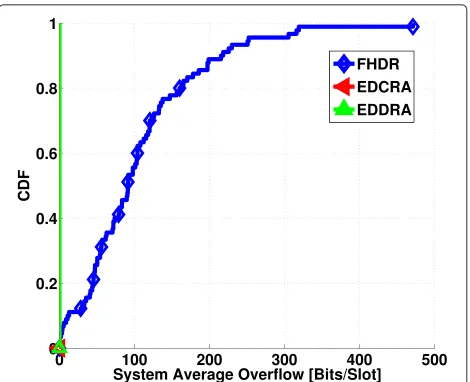
We note that due to limited buffer capacities, all the queues are stable and their sizes are less than the corre-sponding buffer capacities. Therefore, in the following, we do not present any results about them and instead study the overflow performance. Figure 5 displays the cumula-tive distribution function (CDF) of the system utility. It is observed that all the algorithms have the same util-ity of data admissions. This indicates that all of them lead to similar amount of transmissions from the BS, and therefore, similar queue sizes in it which allow sim-ilar data admissions. However, as shown in Fig. 6, the
Fig. 5CDF of system utility at the data arrival rate of 20 packets/s
Fig. 6CDF of system average overflow at the data arrival rate of 20 packets/s
total overflow from the buffers of relays is zero with the proposed EDCRA and EDDRA schemes whereas FHDR has the incidents of overflow. This is due to the fact that FHDR does not take into account the limited buffer capac-ities of the relays when deciding about the subchannel allocations. On the contrary, in the case of insufficient free space in a relay buffer, the proposed schemes do not allo-cate any subchannel to the corresponding link from the BS and this way, they prevent data transmissions to that buffer.
We have also presented the system average through-put, received by the users, in Fig. 7. It is observed that the EDCRA and EDDRA result in higher throughput than

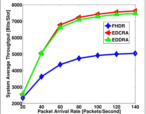
![Fig. 15 Effect of value parameter V on the system utility in the settingsof [21]](https://thumb-us.123doks.com/thumbv2/123dok_us/944071.1115106/19.595.306.540.509.699/fig-effect-value-parameter-v-utility-settingsof.webp)
