Global dynamics of a state dependent feedback control system

R E S E A R C H

Open Access

Global dynamics of a state-dependent

feedback control system

Sanyi Tang

_{, Wenhong Pang}

_{, Robert A Cheke}

_{and Jianhong Wu}

*_{Correspondence:} sytang@snnu.edu.cn 1_{School of Mathematics and} Information Science, Shaanxi Normal University, Xi’an, 710062, P.R. China

Full list of author information is available at the end of the article

Abstract

The main purpose is to develop novel analytical techniques and provide a comprehensive qualitative analysis of global dynamics for a state-dependent feedback control system arising from biological applications including integrated pest management. The model considered consists of a planar system of differential equations with state-dependent impulsive control. We characterize the impulsive and phase sets, using the phase portraits of the planar system and the Lambert W function to define the Poincaré map for impulsive point series defined in the phase set. The existence, local and global stability of an order-1 limit cycle and obtain sharp sufficient conditions for the global stability of the boundary order-1 limit cycle have been provided. We further examine the flip bifurcation related to the existence of an order-2 limit cycle. We show that the existence of an order-2 limit cycle implies the existence of an order-1 limit cycle. We derive sufficient conditions under which any trajectory initiating from a phase set will be free from impulsive effects after finite state-dependent feedback control actions, and we also prove that order-k(k≥3) limit cycles do not exist, providing a solution to an open problem in the integrated pest management community. We then investigate multiple attractors and their basins of attraction, as well as the interior structure of a horseshoe-like attractor. We also discuss implications of the global dynamics for integrated pest management strategy. The analytical techniques and qualitative methods developed in the present paper could be widely used in many fields concerning state-dependent feedback control.

MSC: 34A37; 34C23; 92B05; 93B52

Keywords: planar impulsive semi-dynamical system; integrated pest management; Poincaré map; impulsive set; phase set; global stability

1 Introduction

This study concerns the global dynamics of semi-dynamical systems with state-dependent feedback arising from modeling integrated pest management (IPM) [–]. The challenge for the study of the system’s global dynamics is due to the state-dependent impulsive con-trol.

Impulsive semi-dynamical systems arise from many important applications in the life sciences including population dynamics (biological resource and pest management pro-grams, and chemostat cultures) [–], virus dynamics (HIV) [–], medicine and phar-macokinetics (diabetes mellitus and tumor control) [–], epidemiology (vaccination strategies, the control of epidemics and plant epidemiology) [–], and neuroscience

[–]. In some applications such as spraying pesticides and releasing natural enemies for pest control and impulse vaccinations and drug administrations for disease treatment [–, , , ], the impulsive control is implemented at fixed moments to reflect how human actions are taken at fixed periods. In some applications, however, impulsive differ-ential equations with state-dependent feedback control have to be used to model density-dependent control strategies [, , , , , ]. In particular, in an integrated pest manage-ment (IPM) strategy, actions are taken only when the density of pests reaches an economic threshold [, ]. Feedback control strategies have also been applied in different fields in quite different ways [–].

There has also been substantial theoretical development for impulsive semi-dynamical systems [–]. Techniques including the Lyapunov method have been developed to study the stability and boundedness of solutions for impulsive differential equations with fixed moments, with applications in many important areas [–, ]. Despite a few inter-esting studies on more complicated dynamics such as limit cycles [–], invariant and limiting sets [–], LaSalle’s invariance principle [] and the Poincaré-Bendixson the-orem [, ], much remains to be done for the qualitative theory, and especially the global dynamics, of impulsive semi-dynamical systems. This is particularly so for impulsive dif-ferential equations with state-dependent feedback control.

Some prototype models with biological motivation are needed to guide the development of a general qualitative theory of semi-dynamical systems with state-dependent control. A good example in the series of models motivated by integrated pest management (IPM) [–], where the classical Lotka-Volterra model with state-dependent feedback control is used and some novel techniques for the existence and stability of an order- limit cycle, non-existence of limit cycles with order no less than , the coexistence of multiple attrac-tors and their basins of attraction are developed. The modeling framework and the de-veloped analytical techniques have been used in a number of recent studies. For example, Huanget al.[] proposed mathematical models depicting impulsive injection of insulin for type  and type  diabetes mellitus, and considered the existence and local stability of an order- limit cycle. Based on biomass concentration-dependent impulsive perturba-tions, the studies [, ] proposed and analyzed chemostat models with state-dependent feedback control, again focusing on the existence and stability of an order- limit cycle. These studies also found that the models have no limit cycles with order no less than . The work [, ] also considered the existence and stability of limit cycles with different orders, in relation to the biological issue of maintaining the density of an infected plant population below a certain threshold level. See also similar work on population dynamics [, , –] and epidemiology []. These studies, however, focused on the existence and local stability of an order- limit cycle for specific cases.

Here, we develop novel analytical techniques in order to understand the global dynamics of a very general class of impulsive models with state-dependent feedback control, com-monly used in a number of biological applications including IPM. In particular, we address the following issues and explore their biological implications:

• the precise information as regards the domains of impulsive sets and the phase sets, and the domains for the Poincaré map of impulsive point series;

• the global stability of order- limit cycles (including boundary order- limit cycles); • the existence of order- limit cycles and non-existence of limit cycles with order no

• the necessary condition for the existence of order- limit cycles, and the relation between the existence of order- limit cycles and order- limit cycles;

• the precise information on parameter space for the finite state-dependent feedback control actions, crucial for designing threshold control strategies;

• the description of smaller attractors, their basins of attraction and how they are related to phase sets and interior structures of horseshoe-like attractors.

2 The model with state-dependent feedback control

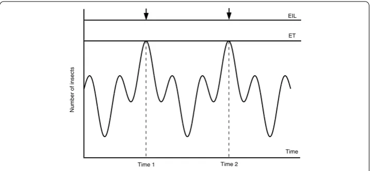
A threshold policy can be defined in broad terms as follows: control (grazing, harvesting, pesticide application, treatmentetc.) is suppressed when a specific species abundance is below a previously chosen threshold density; above the threshold, control is applied. Its application can be seen in wide areas. For an IPM strategy, a long-term management strat-egy that uses a combination of biological, cultural, and chemical tactics to reduce pests to tolerable levels, actions must be taken once a critical density of pests (economic threshold, ET) is observed in the field so that the economic injury level (EIL) is not exceeded [, , ], as shown in Figure . Note that EIL and ET are important components of a cost effec-tive IPM program and are useful for decision-making in the applications of pesticides [, ]. For chemostat setting, when the lactic acid concentration in the bioreactor reaches the critical level, the appropriate control measures (extraction, dilutedness,etc.) should be used such that the concentration of the substrate and the lactic acid change instanta-neously []. Similarly, once the concentration of the tumor cells reaches the therapeutic threshold level in tumor tissue, a combination of photodynamic therapy and sonodynamic therapy should be used [–]. Moreover, including CD+_{T cell counts and/or viral load} level, state-dependent guided antiretroviral therapy has been widely used in HIV [–], hepatitis B virus, and hepatitis C virus treatment [, –].

Letxandybe the densities of the pest and its natural enemy populations. The integrated control interventions are implemented once thexgrows and reaches the threshold level. Denoting the threshold level asVL, the state-dependent impulsive differential equations

are

⎧ ⎪ ⎪ ⎪ ⎪ ⎨ ⎪ ⎪ ⎪ ⎪ ⎩

dx(t)

dt =rx(t)[ –x(t)/k] –ax(t) –px(t)y(t), dy(t)

dt = cx(t)y(t)

+ωx(t) –qx(t)y(t) –δy(t),

x<VL,

x(t+_{) = ( –θ)x(t),} y(t+_{) =y(t) +τ,}

x=VL,

(.)

where x(t+_{) andy(t}+_{) denote the numbers of pests and natural enemies after a control} strategy applied at timet, andx(+_{) andy(}+_{) denote the initial densities of pest and} nat-ural enemy populations. Throughout this paper we assume that the initial density of the pest population is always less thanVL,i.e. x(+_{) =x}

<VL,y(+) =y> . Otherwise, the initial values are taken after an integrated control strategy application.

For the model without control strategy in (.),rrepresents the intrinsic growth rate of the pest population,krepresents the carrying capacity. The pest population dies at a rateaxand is predated by the predator population at a ratepxy. The predator response expands at a rate _+cxy_ωx, which is a saturating function of the amount of pest present. The prey population also inhibits the predator response at a rateqxy, which is the so-called anti-predator behavior, and in the absence of the pest declines at a rateδy. Note that all parameters shown in model (.) are non-negative constants.

Many experiments show that the predator and prey populations can reverse their roles, whereby adult prey attack vulnerable young predators [–], the so called anti-predator behavior. If the variablesxandyin model (.) describe the prey and predator populations, then the termqxyrepresents the effects of the prey population on the predator popula-tion,i.e.the prey can kill their predators. Simple predator-prey models with anti-predator behavior have been studied [, ].

In model (.) ≤θ<  is the proportion by which the pest density is reduced by killing or trapping once the number of pests reachesVL, whileτis the constant number of natural enemies released at this timet. Different releasing methods including a proportion for the release rate rather than a constant number can be used in model (.) [, , ]. In order to control the pest we assume, throughout the paper, that τ ≥b_p ifθ =  (from a biological point of view, sufficient of the natural enemies must be released to prevent the pest population exceedingVL,i.e., by maintaining dx_dt(t) <  (for some time) andθ >  if

τ = . Such a strategy ensures thatx(t) is a decreasing function of time once the pest population reaches theVL.

It is interesting to note that this model can be commonly used in depicting (i) the anti-predator behavior of the interaction between pest and its natural enemies, as shown above; (ii) the interaction between the virus population (such as HIV) and its immune cells []; (iii) the cytotoxic T lymphocyte response to the growth of an immunogenic tumor []; and (iv) the interaction between a toxic phytoplankton population and a zooplankton pop-ulation [, ].

inves-tigate the qualitative behavior of model (.), of particular interest in the dynamics listed in the Introduction.

Note that this work will focus on model (.) with state-dependent feedback control, aiming to maintain the density ofxbelow the previous given threshold level. Thus, it is reasonable to assume that the populationxcould grow exponentially before reaching the threshold level as the threshold value is relatively small compared with the carrying ca-pacity,i.e.we can letk→+∞, then model (.) becomes

Some special cases of model (.) have been investigated [, , ]. For example, letω=  andq= , then model (.) becomes

which has been investigated by Tang and Cheke [], and we will see that all results related to model (.) can be easily obtained based on the results for model (.).

3 The ODE model and its main properties The ODE model considered in this work becomes

It is easy to see that for model (.) there exists a trivial equilibrium (, ) and the interior equilibrium (x∗,y∗) satisfiesy∗=b_p andx∗is the root of the following equation:

Therefore, there are two interior equilibria, denoted by

provided thatc–q–δω>  and= (c–q–δω)_{– qωδ> . Therefore, if}

c–q–δω> qωδ, (.)

then there are two interior equilibriaEandE. Moreover, the two roots collide together if c–q–δω= √qωδ. Throughout this work we assume that the condition (.) holds true. It is easy to show thatEis a saddle point andEis a center.

It follows from model (.) that we have

dy

which implies that model (.) possesses the first integral

H(x,y) = Lambert W function and its properties [] are necessary throughout the paper, for details see the Appendix.

Thus, according to the definition of the Lambert W function and solvingH(x,y) =hwith respect toyyields two roots

yL= –b

Again, according to the domains of the Lambert W function we require

–p

to ensure thatyLandyUare well defined. So we first consider the following equation:

Denote

F(x) =cln( +ωx) –δωln(x)

and

F(x) =qωx–hω+bωln

be– p

.

By simple calculation we have

F_(x) = cω  +ωx–

δω

x , F (x) = –

cω

( +ωx)+

δω

x

and solvingF_(x) =  with respect toxyields the extreme point, denoted byxm=_c–δ_δω, and xm>  holds true due toc–q–δω> .F_(x) =qω. SolvingF_(x) =  yields two inflection points, denoted byx

I andxI, and

x_I=δω+ √

cδω ω(c–δω) , x

 I =

δω–√cδω ω(c–δω)

withx_I <xm<x_I.

Moreover, it is easy to see thatlim_x→+F(x) = +∞, and solvingF

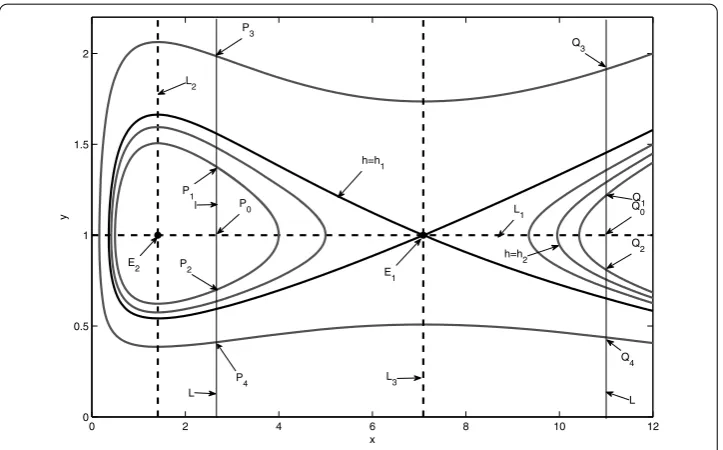
(x) =F(x) with respect toxyields two roots (as shown in Figure ), which are exactly the abscissas of two interior equilibriaEandE,i.e.

x∗_,=c–q–δω±

(c–q–δω)_{– qωδ}

qω .

Denote

h=bln y∗

–py∗_– c

ωln  +ωx

∗ 

+δln x∗_+qx∗_

=bln(b/p) –b– c

ωln  +ωx

∗ 

+δln x∗_+qx∗_

=bln be–/p– c

ωln  +ωx

∗ 

+δln x∗_+qx∗_

and

h=bln y∗

–py∗_– c

ωln  +ωx

∗ 

+δln x∗_+qx∗_

=bln be–/p– c

ωln  +ωx

∗ 

+δln x∗_+qx∗_.

The family of closed orbits is

h=

(x,y)|H(x,y) =h,h<h<h

, (.)

moreover,hconverts to the equilibrium pointEash→h, andhbecomes the homo-clinic cycle ash→h.

Therefore, the two curvesF(x) andF(x) are tangent atx=x_∗orx=x∗_,i.e. h=h or h=h. If we choosehas a bifurcation parameter, then the domains of two branches ofyL andyUcan be determined as follows:

• Ifh<h<h, then there are three intersect points between two functionsF(x)and F(x), denoted byxmin,xmid, andxmax, as shown in Figure . For this case, the two branches ofyLandyUare well defined for allx∈[xmin,xmid]∪[xmax, +∞)with

yL≤b_p ≤yU, as shown in Figure .

• Ifh≤horh≥h, then there exists a unique intersect point between two functions

In particular, ifω=q= , then the model becomes the classical Lotka-Volterra model, and the unique interior (δ/c,b/p) is a center. The first integral is as follows:

The following theorem is useful for discussing the existence of multiple attractors of models with state-dependent feedback control proposed in this work.

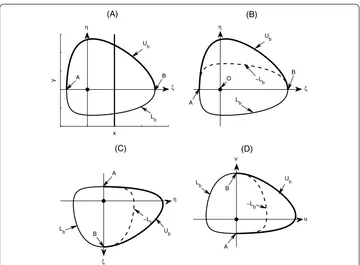
Theorem . Let straight line Lthrough point(x∗,y∗e)be parallel to the x axis,as shown in Figure.Take any point P(or Q)in L,draw the line L through P(or Q),perpendicular to L.Choose a point P(or Q)in L such that|PP|=>  (or|QQ|=> ),and then there exists a unique trajectory of system(.)through point P (or Q)and it intersects another point P (or Q)in L.Then we must have|PP|=≥ |PP| (or|QQ|=≥ |QQ|),where| · |denotes the length of the line segment.Similar results can be had for the trajectory through point P(or Q),as shown in Figure.

Figure 4 Illustration of transformations used in proof of Theorem 3.1.

which implies that

dη

dξ =

–ξ(η+b/p)[–qωξ+ (c–q–δω) – qωx∗_]

pη(ξ+x∗_)( +ω(ξ+x∗_)) F(ξ,η). (.)

Meanwhile, the –Lbshown in Figure (B) satisfies the following scalar differential equa-tion:

dη

dξ =

–ψ(ξ, –η)

φ(ξ, –η) =

–ξ(–η+b/p)[–qωξ+ (c–q–δω) – qωx∗_]

pη(ξ+x∗_)( +ω(ξ+x∗_)) f(ξ,η). (.)

Note that η> , ξ +x∗_> , and (c–q–δω) – qωx∗_=(c–q–δω)_{– qωδ, and it} is easy to know that F(ξ,η) >f(ξ,η) for ξ < ,F(ξ,η) <f(ξ,η) for  <ξ <x∗_ –x∗_ =

(c–q–δω)_{– qωδ/(qω). Further, we haveF(ξ,η)}→ ∞_andf(ξ,η)→ ∞_asη→_. Therefore, if we can show that the curveUblies above the curve –Lbat the right hand side of point A and left hand of point B for all  <η (as shown in Figure (B)), then, according to the comparison theorem of ODE, the whole curve Ub must lie above the whole curve –Lband the results follow. In the following we only prove the curveUblies above the curve –Lbat the right hand side of point A. To do this, we rotate Figure (B)  degrees clockwise about the origin, as shown in Figure (C), and then denoteu=ηand v= –ξ, which yields Figure (D). Consequently, (.) and (.) become

dv du= –

 F(ξ,η)= –

 F(–v,u)

= pu(–v+x ∗

)( +ω(–v+x∗))

and

dv du= –

 f(ξ,η)= –

 f(–v,u)

= pu(–v+x ∗

)( +ω(–v+x∗))

–v(–u+b/p)[qωv+ (c–q–δω) – qωx∗_]G(u,v). (.)

Similarly, at the pointAwe havev<  and  <u, and then  < –u+b/p<u+b/p. Therefore, we haveg(u,v) <G(u,v) for  <u andv< , andg(u,v) =G(u,v) foru=  andv< . So if we choose the initial pointAwith (u,v) = (,v), then according to the second comparison theorem of ODE the results are true.

Corollary . Ifω= and q= ,then model(.)reduces to the classical Lotka-Volterra model,and we conclude that the results shown in Proposition.of reference[]are true.

4 Impulsive set, phase set, and Poincaré map

In order to employ the ideas of the Poincaré map or its successor function to address the existence and stability of order-klimit cycles, we must know the exact conditions under which the solution of model (.) initiating from (x+_,y+_)∈Nis free from impulsive effects, i.e.the more exact phase setN should be provided. Moreover, for the impulsive setM, ≤y≤b_p is the maximum interval for the vertical coordinates ofM. Thus, we also want to know the exact interval,i.e.in which part of ≤y≤b_pthe solution of model (.) cannot reach and then the exact domains of the impulsive set can be obtained.

Based on the position ofVLfor fixedθwe consider the following three cases:

(C) VL≥x∗_; (C) x∗_<VL<x∗_ and (C) VL≤x∗_. (.)

Further, the three quantitiesAh,Ah, andAare useful throughout the rest of the paper,

which are defined as

Ah=

c

ωln

 +ωx∗_  +ω( –θ)VL

–δln

x∗_ ( –θ)VL

–qx∗_– ( –θ)VL

, (.)

Ah= c

ωln

 +ωVL  +ω( –θ)VL

–δln

  –θ

–qθVL (.)

and

A= c

ωln

 +ωx∗_  +ωVL

–δln

x∗_ VL

–qx∗_–VL=Ah–Ah. (.)

Based on the signs ofAh,Ah, andA, we can discuss of the domains of the impulsive

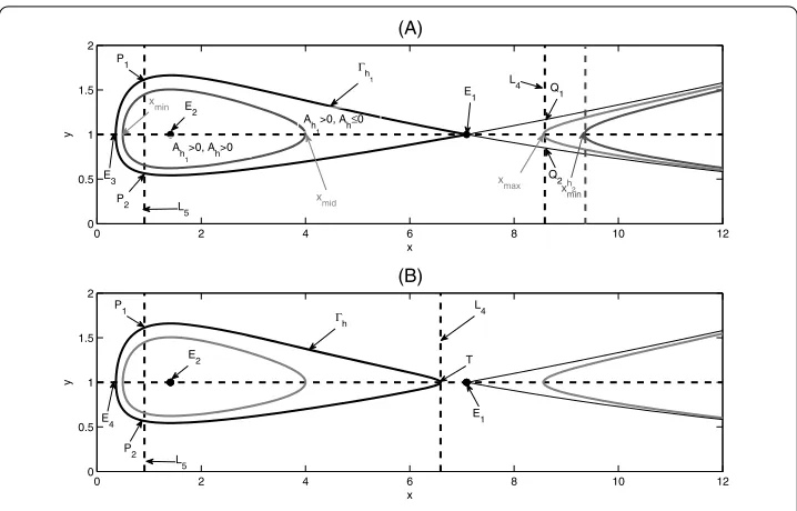
set and the phase set of model (.). To show this, we letx∗_be the horizontal component of the small intersection point (denoted byE= (x∗,b/p)) of the homoclinic cyclehwith

Figure 5 Illustrations of the domains of the impulsive set and the phase set for cases (C1) and (C2). (A)VL≥x∗1andx3∗≤(1 –θ)VL≤x1∗;(B)x∗2<VL<x1∗andx4∗< (1 –θ)VL.

4.1 Impulsive set

There are two subsetsM andM of the basic impulsive setMwhich are needed for providing the exact domains of the impulsive set of model (.), where

M=

(x,y)∈R₊|x=VL, ≤y≤Yish

(.)

and

M=

(x,y)∈R₊|x=VL, ≤y≤Yh

is

, (.)

where

Y_ish= –b pW –e

–+Ah_{b , Y}h

is = – b pW –e

––A

b _(.)

withAh≤ andA≥. Moreover, we haveM=MonceAh= , andM=Monce A= .

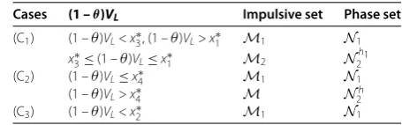
Lemma . For case(C),if( –θ)VL<x∗or( –θ)VL>x∗,then the impulsive set is defined byM; if x∗≤( –θ)VL≤x∗ then the impulsive set is defined byM.For case(C),if ( –θ)VL≤x∗_,then the impulsive set is defined asM;if( –θ)VL>x∗_,then the impulsive set is defined byM.For case(C),the impulsive set is defined byM.

can be determined as follows:

bln(y) –py– c

ωln( +ωx) +δln(x) +qx=bln(b/p) –b–

c

ωln  +ω( –θ)VL

+δln ( –θ)VL+q( –θ)VL. (.)

For this case, the lineL(i.e. x=VL) will intersect with the curveat two points, denoted byQandQ, and the vertical coordinates of both points are the two roots of the following equation:

bln(y) –py=bln(b/p) –b+Ah, (.)

i.e.we have

–p bye

–p_by_{= –e}–+Ah_{b ,}

which can be solved by employing the Lambert W function,i.e.ifAh≤ then we have

Y_ish= –b pW –e

–+Ah_{b , Y}h IS= –

b

pW –, –e

–+Ah_{b . (.)}

Thus, if ( –θ)VL<x∗_, then the impulsive set is defined byM. If so, no solution of model (.) initiating from the phase set can reach into the interval (Y_ish,b/p].

Ifx∗_≤( –θ)VL≤x∗, then the lineLintersects with the right branch of the homoclinic cycleH(x,y) =hat two points, denoted byQ= (VL,YISh) andQ= (VL,Yish) (as shown in Figure ), whereYh

IS andY h

is are two roots of the following equation with respect toy:

bln(y) –py=bln(b/p) –b–A.

Solving the above equation with respect toyyields two roots as follows:

Yh

is = – b pW –e

––A

b _{, Y}h

IS = – b

pW –, –e ––A

b _{. (.)}

Therefore, ifx∗_≤( –θ)VL≤x∗, then the impulsive set can be defined byM. If so, no solution of model (.) initiating from the phase set can reach the interval (Yh

is ,b/p]. If ( –θ)VL>x∗_, then by using the same methods as subcase ( –θ)VL<x∗_the impulsive set is defined byM. Similarly, we can prove the results for case (C) and case (C) are

true.

4.2 Phase set

The exact domains of the phase set depend on the domains of the impulsive set and whether the solution of model (.) initiating from (x+_,y+_)∈N is free from impulsive effects or not. Thus, to discuss the domains of the phase set, we defineY

DandYDrelated to the intervalYD(hereYD= [τ,b/p+τ]) as the following two intervals:

Y_D=τ,Y_ish+τ, Y_D=τ,Yh

is +τ

We first address under which conditions the solution of model (.) initiating from (x+

,y+)∈N will be free from impulsive effects, and then provide the exact domains of the phase set for each case.

Lemma . For case(C),if x∗_≤( –θ)VL≤x∗_,then any solution initiating from(x+_,y+_)∈ N with y+_∈[Yh

min,Y

h

max]will be free from impulsive effects,where

Yh min= –

b pW –e

––Ah_b_{, Y}h max= –

b

pW –, –e

––Ah_b_{. (.)}

Moreover,x∗_< ( –θ)VL<x∗_⇔Ah> ,and Ah= at( –θ)VL=x∗and( –θ)VL=x∗.

Proof Note that the curve of homoclinic cyclehcan be described as follows:

h: H(x,y) =bln(y) –py–

c

ωln( +ωx) +δln(x) +qx=h. (.)

Substitutingy=b/pinto the above equation, one can see thatx∗_ satisfies the following equation:

F(x)=. c

ωln

 +ωx∗_  +ωx

–δln

x∗_ x

–q x∗_–x= .

Taking the derivative ofF(x) with respect toxyields

F_(x) = – c

 +ωx+q+

δ

x

and solving F_(x) =  yields two rootsx=x∗_ andx=x∗_. It is easy to see thatF(x∗_) = F_(x∗_) = . This indicates thatF(x) >  for allx∈(x∗_,x∗_)∪(x∗_, +∞).

In this case, the lineLmust intersect with the homoclinic cyclehat two points,

de-noted byP= (( –θ)VL,Ymaxh ) andP= (( –θ)VL,Yminh ), which are the two roots of (.)

with respect toyforx= ( –θ)VL. In fact, substitutingx= ( –θ)VLinto (.) and rear-ranging it yield

bln(y) –py=bln(b/p) –b–Ah,

i.e.we have

–p bye

–p_by_{= –e}––Ah_b_.

Solving the above equation with respect toyyields two roots which are given by (.). Moreover, both P andP are well defined due to Ah =F(( –θ)VL)≥ for allx∗ ≤ ( –θ)VL≤x∗. Thus, any trajectory initiating from (x+,y+)∈N withY

h

min≤y+≤Y h maxwill

be free from impulsive effects.

Therefore, for case (C) (i.e. VL≥x∗_), ifx∗_≤( –θ)VL≤x∗_, the phase set can be defined as follows:

Nh

 = x+,y+

∈R₊|x+= ( –θ)VL,y+∈Yh

D

with

Yh

D =

,Yh min

∪ Yh max, +∞

∩Y_D. (.)

If ( –θ)VL<x∗_or ( –θ)VL>x∗_, then the phase set for model (.) is defined as

N= x+,y+

∈R₊|x+= ( –θ)VL,y+∈Y_D. (.)

Moreover, any solution initiating from phase set N will experience infinite state-dependent feedback control actions.

Lemma . For case(C),if x∗_< ( –θ)VL,then any solution initiating from(x+

,y+)∈N with y+

∈(Yminh ,Ymaxh )will be free from impulsive effects,where

Yminh = –

b pW –e

––Ah_{b , Y}h

max= –

b

pW –, –e

––Ah_{b . (.)}

Moreover,x∗< ( –θ)VL⇔Ah> ,and Ah= at( –θ)VL=x∗.

Proof The closed orbithforh<h<hwhich is contained inside the pointEand tan-gent to the lineLcan be determined as follows:

h: H(x,y) =bln(y) –py– c

ωln( +ωx) +δln(x) +qx=h (.)

withh=bln(b/p) –b–_ωcln( +ωVL) +δln(VL) +qVL.

Similarly, substitutingy=b/pinto the above equation, one can see thatx∗_should be the smallest root of the following equation:

F(x)=. c

ωln

 +ωVL  +ωx

–δln

VL x

–q(VL–x) = .

Moreover, we haveF_(x∗_) =F_(x_∗) = . This indicates thatF(x) >  for allx∈(x∗_,VL). Further, the lineLmust intersect withhat two points, denoted byP= (( –θ)VL,Ymaxh )

andP= (( –θ)VL,Yminh ), which are the two roots of (.) with respect toyforx= ( –

θ)VLand can be obtained by using the same methods as those in the proof of Lemma .. Moreover, bothPandPare well defined due toAh=F(( –θ)VL)≥ for allx∗≤( –

θ)VL. Therefore, any trajectory initiating from (x+,y+)∈N withYminh <y+<Ymaxh will be

free from impulsive effects.

Therefore, for case (C) (i.e. x∗<VL<x∗), ifx∗< ( –θ)VL, then the phase set can be defined as follows:

Nh

 = x+,y+

∈R₊|x+= ( –θ)VL,y+∈Y_Dh (.)

with

Y_Dh=,Yminh

∪Ymaxh , +∞

Table 1 Exact domains of the impulsive set and phase set of model (2.2)

Cases (1 –θ)VL Impulsive set Phase set

(C1) (1 –θ)VL<x3∗, (1 –θ)VL>x∗1 M1 N1

x∗₃≤(1 –θ)VL≤x∗1 M2 N2h1

(C2) (1 –θ)VL≤x∗4 M1 N1

(1 –θ)VL>x4∗ M N2h

(C3) (1 –θ)VL<x2∗ M1 N1

If ( –θ)VL≤x∗_, then the phase set is defined byN. Finally, for case (C), it is easy to see that the phase set for model (.) is defined byN.

In conclusion, we list all possible cases for the domains of the impulsive set and phase set of model (.) in Table . It follows that the basic phase setNcannot be used to define the real phase set of model (.) for any case. This indicates that the exact domains of the phase set of model (.) should be carefully discussed. However, the domains of the impulsive set and phase set have not been discussed carefully in the previous literature [, ], which may result in some difficulties in employing the Poincaré map or its successor function to study the existence and stability of limit cycles of planar impulsive semi-dynamical systems.

In the following, if we consider bothAh andAh as functions ofVL, then we have the

following results.

Lemma . Ah=Ahat VL=x∗ and Ah>Ahif VL>x∗. Proof It is easy to see that

F(VL)=. Ah–Ah=

c

ωln

 +ωx∗_  +ωVL

–δln

x∗_ VL

–qx∗_–VL=. A. (.)

Based on the proof of Lemma . we can see that the equationF(VL) =  with respect to VLhas two rootsVL=x∗_andVL=x∗_. It follows fromF(x∗_) =F(x∗_) =  thatAh>Ahfor

allVL>x∗.

The impulsive set and phase set for model(.). Letx∗_be the horizontal component of the small intersection point (denoted by E= (x∗,b/p)) of the closed trajectory h

which is contained inside the center (δ/c,b/p) and is tangent to the lineL at pointT withT= (VL,b/p). It follows from the first integral (.) that the closed cycle initiating from (VL,b/p) satisfies

bln(y) –py+δln(x) –cx=bln(b/p) –b+δln(VL) –cVL.

Substitutingy=b/pinto the above equation, one can see thatx∗_satisfies

δln(x) –cx=δln(VL) –cVL,

solving it with respect toxwe get two roots: one isVLwithVL≥δ_cand the other is given by

x∗_= –δ cW

–cVL

δ exp

–cVL

δ

Thus, by using the same methods as those in the proof of Lemma . we have the fol-lowing results for model (.).

Lemma . For the case VL>δ/c in model(.).If x∗_< ( –θ)VL,then any solution of model(.)initiating from(x+_,y+_)∈N with y+_∈[Ymin ,Ymax ]will be free from impulsive

effects,where

Ymin = –

b pW –e

––A_b_{, Y}

max= –

b

pW –, –e

––A_b _(.)

and

A=cθVL–δln

  –θ

. (.)

Moreover,x∗_< ( –θ)VL⇔A> and A= at VL= x∗_ –θ.

The impulsive set of model (.) can be determined as those for model (.), and we only need to consider two cases,i.e. VL>δ/candVL≤δ/c. For the former case, if ( –θ)VL<δ/c then the impulsive set is defined byM_ and

M  =

(x,y)∈R₊|x=VL, ≤y≤Y_is (.)

with

Y_is= –b pW –e

–+A_b_{. (.)}

If ( –θ)VL≥δ/cthen the impulsive set isM. For the latter case (i.e. VL≤δ/c), it is easy to see that the impulsive set is defined byM_.

Therefore, ifVL>δ/c, then the phase set for the casex∗_< ( –θ)VLcan be defined as

Nh

 = x+,y+

∈R₊|x+= ( –θ)VL,y+∈Y_Dh (.)

with

Y_Dh=,Ymin

∪Ymax , +∞

∩YD. (.)

The phase set for the case ( –θ)VL≤x∗_is defined byN_and

N

 = x+,y+

∈R₊|x+= ( –θ)VL,y+∈YD

, and Y_D=τ,Y_is+τ. (.)

Finally, ifVL≤δ/c, then it is easy to see that the phase set is defined byN_.

Remark . Before we provide the formula for the Poincaré map of model (.), we want to show how the phase sets change as the key parameters (i.e.θ, VL, and τ) vary. For example, the setNh

 can be defined exactly according to the relations amongτ,Yminh , and

Yh

max. One simple case is as follows: ifτ≤Yminh andYmaxh ≤τ+b/pthen

Nh

 = x+,y+

∈R₊|x+= ( –θ)VL,y+∈Y_DmM=τ,Yminh

∪Ymaxh ,τ+b/p

Similarly, we can discuss several other cases and get the domains ofY_DmMandN_h, where

It follows from Remark . that the relations amongτ,Yh

min, andYmaxh are crucial for the

exact domains of the phase set, which will be addressed later.

4.3 Poincaré map

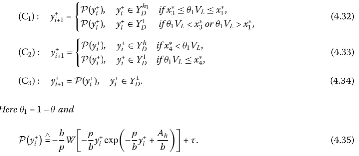
Theorem . The Poincaré map for the impulsive points of model(.)defined in the phase set can be determined as

(C) : y+_i+= impulses k+  times (finite or infinite), we denote the corresponding coordinatesPi= (VL,yi)∈MandP+_i = (( –θ)VL,y+_i)∈N,i= , , . . . ,k. Therefore, if both pointsP+_i and Pi+lie in the same trajectory(closed or non-closed) fori= , , . . . ,k, then the pointsP+i andPi+satisfy the following relation:

c

In order to show the exact domains of the Poincaré map, we first need to know under what conditions the trajectory initiating fromP+

i ∈N cannot reach the pointPi+∈M.

cannot reach the lineL, which shows that both pointsP+_i andPi+cannot lie in the same trajectory, as shown in Figure (B). It follows from Lemma . and Table  again that in this case we haveAh>  and we requireP+

Solving the above equation with respect toyi+, we have

yi+= –

this indicates that equation (.) is well defined in this case. If Ah> , we must have –p_by+_i exp(–p_by+_i +Ah

Ahand according to the monotonicity of the Lambert W function we have [Yh

min,Ymaxh ]⊂ haveAh< , consequently the Poincaré map is given by the second case of (.).

The other two cases (C) and (C) of Theorem . can be obtained directly from the domains of the Poincaré map and the proof of Lemma .. This completes the proof.

It follows from Lemma . that we have the main results for the Poincaré map of the impulsive points of model (.).

Corollary . The Poincaré map for the impulsive points of model(.)defined in the phase set can be determined as

y+_i+=

Compared with published definitions of the Poincaré map for model (.) [, ], we can see that more accurate domains have been provided in formula (.).

Based on the proofs of Lemmas .-. and Theorem . we can see that the signs ofAh

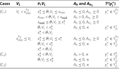
Table 2 The relations among the key parameters (i.e.θ,VL, andτ), the signs ofAh1andAh

and in defining the Poincaré mapP(y+_i). Therefore, the relations among the key parameters (i.e.θ,VL, andτ), the signs ofAhandAhand the domains of the Poincaré mapP(y

+ i) will be discussed briefly before we address the existence and stability of the limit cycle of model (.), which are also important in the rest of this work.

To do this, we take the notations shown in Figure , wherexh

minrepresents the

intersec-tion point of the curveH(x,y) =hwith the liney=b/p. Then the relations among the key parameters (i.e.θ,VL, andτ), the signs ofAhandAhand the domains of the Poincaré map

P(y+

i) can be summarized in Table .

5 Existence of order-1 limit cycles and some important relations

Investigations of the existence and stability of order- limit cycles of system (.) for the whole parameter space are quite challenging, and are similar to the study of the existence and stability of limit cycles of continuous semi-dynamical systems. Fortunately, the ana-lytical formula of the Poincaré map defined by the impulsive points in the phase set has been obtained, which allows us to employ it to study the existence and stability of order- limit cycles of model (.).

The fixed point of the Poincaré mapP(y+

i) in the phase set corresponds with the exis-tence of the order- limit cycles of model (.) and model (.). Without loss of generality, we first discuss the existence of a fixed point of the Poincaré mapP(y+

i) in the basic phase setN,i.e. y+

i ∈YD, and then we will focus on the particular domains of the Poincaré map P(y+_i) in phase sets and discuss the existence of the fixed point. Denote the fixed point asy∗, then we have

Therefore, according to the definition of the Lambert W function the above yields

Note that ifτ=  andAh= , then for any ≤y∗≤b/pthe above equation holds true; if

τ =  andAh= , theny∗=  is a unique fixed point of Poincaré mapP(y+

i). Ifτ> , then solving the above equation with respect toy∗yields

y∗=τ exp(

The necessary condition for the existence of a fixed point of the Poincaré mapP(y+_i) in the phase set is y∗∈YD. Thus, it is interesting to show under what conditions they∗∈

Rearranging the above inequality yields

–p

Solving the above inequality with respect toτ+b_pyieldsτ+b_p≤Yminh (which is impossible

due toYminh <bp) orτ+ basic phase set (i.e. y∗∈YD). To address this and reveal all possible dynamic behavior of model (.), we first need to investigate some important relations amongy∗,y∗_,τ+b/p,

to address the relations,i.e.we considery∗,y_∗,τ+b/p,Ymini ,Ymaxi fori=h,handτ+Yish as functions ofτ. As the first step, we discuss the monotonicity of they∗, wherey∗is given by (.), and we have the following results.

Lemma . If <Ah<pτ,then y∗reaches its minimal value(denoted by y∗minand y∗min=

Yh

max)atτM=Ymaxh –bp.

Proof Taking the derivative ofy∗with respect toτyields

dy∗

Rearranging the above equation yields

–

and it is easy to see thatAh<pτis a necessary condition for the existence of a positive root of the above equation with respect toτ. Solving the above equation with respect toτ, one has two roots and only the larger one is positive, denoted byτM, where

τM= –

Furthermore, it follows from Theorem . that

Rearranging the above inequality yields

b+b_+p_τ_–pτexp

p bτ

–b–pτ–b_+p_τ_{> . (.)}

Denotez=p_bτ> , then the above inequality is equivalent to

ez> + √

 +z_+z  +√ +z_–z=z+

√  +z_.

LetF(z) =ez_{– (z+}√_{ +z}_{) and we have}

F(z) >  +z+ z

_{– z+}√_{ +z}_{=  +}  z

_–√_{ +z}_{> .}

To discuss the relations amongy∗,τ+b/p,Yh

max, andYminh which will be used in this work,

we define the following four functions with respect toτ

 τ . =τ+b

p–y

∗_,  τ .

=y∗–Yh

max, τ .

=y∗–y∗_, τ .

=y∗–Yh

min. (.)

For the first equationτ .

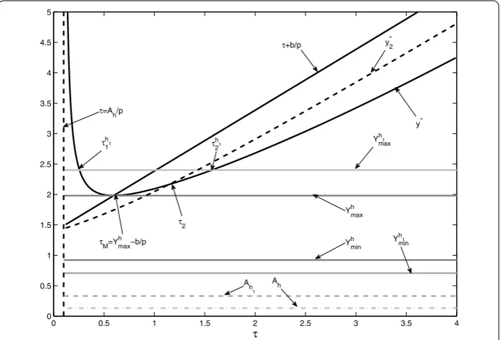
=τ+b_p–y∗= , substitutingy∗into it and arranging the items we can see which is equivalent to the equationτ =  (defined by (.)). This indicates that the equationτ =  has a unique positive rootτM,i.e.the two curvesy∗andτ+b/pwith respect toτ intersect atτ=τM, as shown in Figure .

Figure 6 The relations amongy∗,y∗₂,τ+b/p,Yi

min,Ymaxi andi=h,h1.All other parameter values are fixed

Substitutingy∗into the second function and letting

Rearranging the above equation, one has

p

b _{) into the right hand side of the above equation}

ac-cording to the equationW(z)eW(z)_=zyields

In order to ensure (.) has a positive root with respect toτ, the necessary condition isτ<Yh

max. Given this and according to the definition of the Lambert W function we can

solve it and yield two roots, denoted byτh

 andτ

minat another point, which will be discussed later.

For the third function

τ, we want to find the root of equationτ .

=y∗–y∗_=  with respect toτ,i.e.the positive root of the following equation:

τ exp(

Finally, we discuss the existence of the positive root of the equation

min=  there exists a unique positive

root, denoted byτh

iswhenAh≤. That is, we have the following main results.

Lemma . If A≥,then y∗<τ+Yishfor allτ>τ

which indicates that those three functions (i.e. y∗,Yh

max, andτ+Y_ish) with respect toτ

inter-For the second part of Lemma ., it follows from (.) that we consider the following equation:

with respect toτ. Rearranging the above equation one has

(b–pτ)exp

and solving the above equation one gets the unique positive root whenAh≤

τT=

is) are tangent atτ=τT. According to the monotonicity of both functions we conclude thaty∗≤τ+Y_ishwhenAh≤ and the equal holds true only atτ =τT.

5.2 Existence of order-1 limit cycle

In order to provide the detailed sufficient conditions for the existence of a fixed point of the Poincaré mapP(y+

i), we rearrange the subcases of the cases (C)-(C) according to the domains of the Poincaré mapP(y+

Poincaré mapP(y+_i) defined byY

D(or the phase set defined byNorAh≤) in together, denoted by subcase (SC),i.e.

(SC) : (C) withθVL<x∗orθVL>x∗, (C) withθVL≤x∗and (C). (.)

We denote the subcase for (C) withAh>  andAh≥ as subcase (SC),i.e.

(SC) : (C) withVL<xh

minandxmin<θVL<xmid, (.)

and denote all subcases for (C) withAh≤ andAh≥ as subcase (SC),i.e.

(SC) :

(C) withVL<xh

minandx∗≤θVL≤xmin,

(C) withVL<xh

minandxmid≤θVL≤x∗,

(C) withxhmin ≤VLandx∗≤θVL≤x∗.

(.)

The combination of (SC) and (SC) is called (SC) in this work. Finally, we denote the subcases for (C) withAh>  as subcase (SC),i.e.

(SC) : (C) withx∗_<θVL. (.)

Based on the important relations discussed before, for the existence of a fixed point of the Poincaré mapP(y+_i) of model (.) and consequently the existence of the order- limit cycle we have the following main results.

Theorem . Ifτ= and Ah=  (hereθ> ),then any y∗in the phase set is a fixed point of the Poincaré mapP(y+_i).Ifτ = and Ah= ,then y∗= is a unique fixed point of the Poincaré mapP(y+_i).

Ifτ> ,then the fixed point y∗of the Poincaré mapP(y+

i)is always well defined for(SC) with y∗∈Y

D.Ifτ>τ h

 ,then the fixed point y∗of the Poincaré mapP(y+i)exists for(SC) and y∗∈(Yh

max,Y_ish+τ].If <τ <τ_h(orτ>τ_h),then the fixed point y∗of the Poincaré

mapP(y+_i)exists for(SC)and y∗∈(,Yh

min) (or y∗∈(Y

h

max,Y_ish+τ]).Ifτ ≥τM,then the fixed point y∗of the Poincaré mapP(y+_i)exists for(SC)and y∗∈[Ymaxh ,bp+τ].

Proof The results forτ =  are true obviously. SinceAh≤ for (SC), it follows from Lemma . thaty∗≤τ+Y_ishfor allτ> , which indicates thaty∗exists in the phase set,i.e. y∗∈Y

D. Ifτ>τh

 , then it follows from the relations betweeny∗andY h

maxthaty∗>Ymaxh . Further,

according to Lemma . we havey∗<Yh

is +τ for allτ>τ h

 due toA≥ in case (SC). Thus the fixed pointy∗of the Poincaré mapP(y_i+) exists for (SC) andy∗∈(Yh

max,Y_ish+τ].

If  <τ<τh

 , then it follows from the relations betweeny∗andY h

minthaty∗<Y

h min, which

means that the fixed pointy∗of the Poincaré mapP(y+

i) exists for (SC) andy∗∈(,Yminh ).

Ifτ >τh

 , then the result can be proved by using the same methods as those for case (SC). Ifτ≥τM, then it follows from the relations betweeny∗andYmaxh and the relations

be-tweeny∗ and b_p +τ thaty∗∈[Yh

max,bp +τ] and consequently the last part of the results

shown in Theorem . are true.

Corollary . Assumeτ> .The Poincaré mapP(y+_i)does not have a fixed point for case (SC)providedAh

p <τ≤τ h

 ;The Poincaré mapP(y+i)does not have a fixed point for case (SC)providedτh≤τ≤τ

h

 ;The Poincaré mapP(y+i)does not have a fixed point for case (SC)providedAh

p <τ<τM.

Theorem . and Corollary . provide the detailed conditions for the existence and non-existence of a fixed point of the Poincaré mapP(y+_i) of model (.), consequently the existence and non-existence of order- limit cycles of model (.) can be obtained directly. For the existence and non-existence of a fixed point of model (.) we have the following results.

Corollary . Ifτ = and A=  (hereθ > ),then any y∗ in the phase set is a fixed point of the Poincaré mapP(y+_i)of model(.).Ifτ= and A= ,then y∗= is a unique fixed point of Poincaré mapP(y+_i).Ifτ> and A≤,then for the Poincaré map defined in the phase set there exists a unique fixed point y∗∈Y

D.If A> andτ ≥τM,then for the Poincaré mapP(y+_i)there exists a unique fixed point y∗ with Ymax ≤y∗≤τ +bp.The Poincaré mapP(y+

i)does not have a fixed point provided <Ap <τ<τM.

6 Local and global stability of order-1 limit cycle

To address the stability ofy∗, we note that ifτ=  andAh=  (hereθ> ), theny∗is stable but not asymptotically stable. For the caseτ =  andAh=  (i.e. y∗= ) we will address it as a special case later in more detail. Thus, we first assume thatτ>  andy∗exists, and we provide the sufficient conditions for the local stability and global stability of the fixed pointy∗. Consequently, the global stability of the order- limit cycle of model (.) can be obtained, which improved on previous results on models with state-dependent feedback control [, ].

6.1 Local stability of order-1 limit cycle

Theorem . Assume thatτ> and y∗exists.If Ah≤then the fixed point y∗of Poincaré mapP(y+

i)is locally stable;If Ah> then the fixed point y∗of Poincaré mapP(y+i)is locally stable provided

y∗<b+pτ+

b_+p_τ

p . (.)

Proof For convenience, denotef(y) = –p_byexp(–p_by+Ah

b ), and we have

f(y) = –p bexp

–p by+

Ah b

 –p by

.

Moreover, by simple calculation and according to the properties of the Lambert W func-tion we have

dP(y+_i) dy+_i

y+_i=y∗ = –b

p

W(f(y∗)) f(y∗)( +W(f(y∗)))f

_(y∗₎

= –b p

W(f(y∗))  +W(f(y∗))

 y∗ –

p b

=(y

∗_{–τ)(b–py}∗₎

y∗(b–p(y∗–τ))g(y

We first note that ify∗=τ+b/ptheng(y∗) = –∞, which indicates thaty∗is unstable. Thus, for the stability ofy∗, we only need to focus on the intervalτ <y∗<τ+b/p. Moreover, |g(y∗)|<  is equivalent to the following inequalities:

– <(y

∗_{–τ)(b–py}∗₎

y∗(b–p(y∗–τ))< , (.)

which indicates that if the above inequalities hold, then the fixed pointy∗is locally stable. Note that we havey∗(b–p(y∗–τ)) >  for allτ <y∗<τ+b/pandτ> . It is easy to show that the right hand side of (.) holds true naturally, and the left hand side inequality is equivalent to

p y∗– (b+pτ)y∗+bτ

 <  (.)

and solving the above inequality we havey∗_<y∗<y∗_where

y∗_,=b+pτ∓

b_+p_τ

p .

Further, we can show that

y∗_<τ<y∗_<τ+b/p.

This indicates that ifτ<y∗<y_∗, then the fixed pointy∗of Poincaré mapP(y+

i) is locally stable. It follows from Lemma . thaty∗<y∗_holds true naturally ifAh≤. This completes

the proof of Theorem ..

Corollary . Assume thatτ> ,y∗exists,and Ah> .If y∗∈(y∗_,τ +b_p],then the fixed point y∗of the Poincaré mapP(y+

i)of model(.)is unstable.

Corollary . Assume thatτ > and y∗ exists.If A≤,then the fixed point y∗ of the Poincaré mapP(y+_i)of model(.)is locally stable;If A> ,then the fixed point y∗ of Poincaré map P(y+_i)is locally stable provided y∗ ∈(τ,y∗_),and it is unstable when y∗ ∈ (y∗_,τ+b_p].

By combining Theorems . and ., Corollaries . and ., and all of the relations dis-cussed in Section . we can provide the exact conditions for the existence and stability of the fixed pointy∗of the Poincaré mapP(y+

i) of model (.) based on the three parameters

θ,VL, andτ. Here for simplification and convenience we employ the signs ofAh andAh

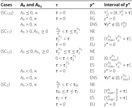
rather thanθ andVL, and list all results in Table .

Here,×means the sign ofAh is not necessary for that subcase, NE denotes the

non-existence of a fixed point, EU represents the non-existence of a fixed point which is unstable, ES shows the existence of a fixed point which is stable, EG denotes the existence of a fixed point which is globally stable, and ENS represents the existence of a fixed point which is neutrally stable. Note that ifτ = , then for case (SC) we haveYh

min=Y

h

is onceAh= . Thus, in this subcase, anyy∗∈[,Yh

min) = [,Y

h